Returning to the problem of having the same patterns at x and x + p. As indicated in eq. (2.21), here it has

$E\left[S_t\left(x;t_i\right)\right]=E\left[S_t\left(x;t_i+\frac{p}{B_i\lambda }\right)\right]=2N_W{\sigma }_n^2\left(2.30\right)$

Note that the uncertainty problem still exists, as the minimum occurs at tp = ti + p/(Biλ). However, with the change of Bi, tp changes but ti does not change. This is an important property of SSSD in inverse-distance. By using such a property, it is possible to select different baselines to make the minima appear at different locations. Taking the case of using two baselines B1 and B2(B1 ≠ B2) as an example, it can be derived from eq. (2.29) that

$\begin{array}{l}E\left[S_{t\left(12\right)}^{\left(S\right)}\left(x;\widehat{t}\right)\right]={{\displaystyle \sum _{j\in W}\left\{f\left(x+j\right)-f\left[x+B_1\lambda \left({\widehat{t}}_1-t_1\right)+j\right]\right\}}}^2\left(2.31\right)\\ +{{\displaystyle \sum _{j\in W}\left\{f\left(x+j\right)-f\left[x+B_1\lambda \left({\widehat{t}}_1-t_1\right)+j\right]\right\}}}^2+4N_W{\sigma }_n^2\end{array}$

It can be proven that when $t\cancel{=}\widehat{t},$ it has Okutomi (1993)

$E\left[S_{t\left(12\right)}^{\left(S\right)}\left(x;\widehat{t}\right)\right]>4N_W{\sigma }_n^2=E\left[S_{t\left(12\right)}^{\left(S\right)}\left(x;t\right)\right]\left(2.32\right)$

This means that at the correct matching location t, there is a real minimum $S_{t(12)}^{(S)}(x,\widehat{t}).$ The uncertainty problem caused by repeated patterns can be solved by using two different baselines.

Example 2.2 The effect of the new measuring function.

One example showing the effect of the new measuring function is illustrated in Figure 2.11, Okutomi (1993). Figure 2.11(a) shows a plot of f(x) given by

$f\left(x\right)=\{\begin{array}{cc}2+\cos \left(x\pi /4\right)& -4<x<12\\ 1& x⩽-4,x\ge 12\end{array}$

Suppose that for baseline B1, it has d1 = 5 and ${\sigma }_n^2=0.2,$ and the window size is 5. Figure 2.11(b) gives E[Sd1(x; d)], which has two minima at d1 = 5 and d1 = 13, respectively. Now, a pair of images with baseline B2 are used, and the new baseline is 1.5 times the old one. Thus, the obtained E[Sd2(x; d)] is shown in Figure 2.11(c), which has two minima at d1 = 7 and d1 = 15, respectively. The uncertainty problem still exists, and the distance between the two minima has not been changed.

Using the SSD in inverse-distance, the curves of E[St1(x; t)] and E[St2(x; t)] for baselines B1 and B2 are plotted in Figure 2.11(d, e), respectively. From these two figures, it can be seen that E[St1(x; t)] has two minima at t1 = 5 and t1 = 13, and E[St2(x; t)] has two minima at t1 = 5 and t1 = 10. The uncertainty problem still exists when only the inverse-distance is used. However, the minimum for the correct matching position (t = 5) has not been changed while the minimum for the false matching position changes with the alteration of the baseline length. Therefore, adding two SSD values in inverse-distances gives the expectation curve $E[S_{t(12)}^{(S)}(x;t)]$ as shown in Figure 2.11(f). The minimum at the correct matching position is smaller than the minimum at the false matching position. In other words, there is a global minimum at the correct matching position. The uncertainty problem is thus solved.

Consider that f(x) is a periodic function with a period T. Every St(x, t) is a periodic function of t with a period T/Biλ. There will be a minimum in every T/Biλ. When two baselines are used, the corresponding $S_{t(12)}^{(S)}(x;t)$ is still a periodic function of t but with a different period T12

$T_{12}=\text{LCM}\left(\frac{T}{B_1\lambda },\frac{T}{B_2\lambda }\right)\left(2.33\right)$

Here, LCM denotes the least common multiple. It is evident that T12 should not be smaller than T1 or T2. By suitably selecting baselines B1 and B2, it is possible to allow only one minimum in the searching region.

2.5Orthogonal Trinocular Matching

One problem often encountered in stereo vision is that mismatching arises for gray-level smooth regions. This problem cannot be solved by the above multiple stereo-matching technique, though it can reduce the mismatching caused by periodic patterns. In real applications, horizontal smooth regions often have visible gray-level differences along the vertical direction. In this case, the mismatching problem caused by the horizontal smoothness can be solved by vertical matching. Similarly, when the region is smooth along the vertical direction, the correct matching could be achieved by a horizontal searching. Considering both vertical and horizontal matching, techniques for the orthogonal trinocular matching are proposed, Ohta (1986).

2.5.1Basic Principles

The basic principles for orthogonal trinocular matching are discussed first.

2.5.1.1Removing Mismatching in Smooth Regions

Since both horizontal smooth regions and vertical smooth regions can appear in real images, both the horizontal pairs and the vertical pairs of images should be captured. In the simplest case, two orthogonal pairs of cameras are arranged in a plane, as shown in Figure 2.12. The left image L and the right image R form the horizontal stereo image pair with baseline Bh. The left image L and the top image T form the vertical stereo image pair with baseline Bv. These two pairs of images form a set of orthogonal trinocular images (the two baselines can have different lengths).

Suppose that the three captured images are

$\begin{array}{l}{f}_L\left(x,y\right)=f\left(x,y\right)+n_L\left(x,y\right)\\ f_R\left(x,y\right)=f\left(x-d_{\text{h}},y\right)+n_R\left(x,y\right)\left(2.34\right)\\ f_T\left(x,y\right)=f\left(x,y-d_{\text{v}}\right)+n_T\left(x,y\right)\end{array}$

where dh and dv are the horizontal and vertical disparities, respectively. In the following discussion, it is assumed that dh = dv = d. The two SSDs respectively corresponding to the horizontal and vertical directions are

$\begin{array}{l}{S}_{\text{h}}\left(x,y;\widehat{d}\right)={\displaystyle \sum _{j,k\in W}{\left[f_L\left(x+j,y+k\right)-f_R\left(x+\widehat{d}+j,y+k\right)\right]}^2}\left(2.35\right)\\ S_{\text{v}}\left(x,y;\widehat{d}\right)={\displaystyle \sum _{j,k\in W}{\left[f_L\left(x+j,y+k\right)-f_T\left(x+\widehat{d}+j,y+k\right)\right]}^2}\end{array}$

Adding them produces the orthogonal disparity measuring function $O^{(S)}(x,y;\widehat{d})$ given by

$O^{\left(S\right)}\left(x,y;\widehat{d}\right)=S_{\text{h}}\left(x,y;\widehat{d}\right)+S_{\text{v}}\left(x,y;\widehat{d}\right)\left(2.36\right)$

The expected value of O(S)(x, y; $\widehat{d}$ ) is

$\begin{array}{l}E\left[O^{\left(S\right)}\left(x,y;\widehat{d}\right)\right]={{\displaystyle \sum _{j,k\in W}\left[f\left(x+j,y+k\right)-f\left(x+\widehat{d}-d+j,y+k\right)\right]}}^2\left(2.37\right)\\ +{{\displaystyle \sum _{j,k\in W}\left[f\left(x+j,y+k\right)-f\left(x+j,y+\widehat{d}-d+k\right)\right]}}^2+4N_W{\sigma }_n^2\end{array}$

where Nw denotes the number of the pixels in the matching window W. From eq. (2.37), when = d

$E\left[O^{\left(S\right)}\left(x,y;d\right)\right]=4N_W{\sigma }_n^2\left(2.38\right)$

E[O(S)(x, y; )] gets its minimum at the position of the correct disparity. It can be seen from the above discussion that to remove periodic patterns in one direction, the inverse-distance is not necessary.

Example 2.3 Removing mismatching in smooth regions by orthogonal trinocular.

Figure 2.13(a–c) represents the left, right, and top images with horizontal and vertical smooth regions. The disparity map obtained by matching horizontal binocular images is shown in Figure 2.13(d). The disparity map obtained by matching vertical binocular images is shown in Figure 2.13(e). The disparity map obtained by matching the orthogonal trinocular images is shown in Figure 2.13(f). In Figure 2.13(d), some visible mismatching occurs at the horizontal smooth region (shown by horizontal strips). In Figure 2.13(e), some visible mismatching occurs at the vertical smooth region (shown by vertical strips). Such mismatching strips have not appeared in Figure 2.13(f). Figure 2.13(g–i) represents 3-D plots corresponding to Figure 2.13(d–f), respectively.

2.5.1.2Reducing Mismatching Caused by Periodic Patterns

The technique of orthogonal trinocular matching can reduce the mismatching caused by smooth regions as well as reduce the mismatching caused by periodic patterns. Consider the case where the object has both horizontal and vertical periodic patterns. Suppose that f(x, y) is a periodic function with horizontal and vertical periods Tx and Ty, respectively, given by

$f\left(x+j,y+k\right)=f\left(x+j+T_x,y+k+T_y\right)\left(2.39\right)$

where Tx and Ty are nonzero constants. From eq. (2.35) to eq. (2.38), the following equations can be derived

$E\left[S_{\text{h}}\left(x,y;\widehat{d}\right)\right]=E\left[S_{\text{h}}\left(x,y;\widehat{d}+T_x\right)\right]\left(2.40\right)$

$E\left[S_{\text{v}}\left(x,y;\widehat{d}\right)\right]=E\left[S_{\text{v}}\left(x,y;\widehat{d}+T_y\right)\right]\left(2.41\right)$

$\begin{array}{l}E\left[O^{\left(S\right)}\left(x,y;\widehat{d}\right)\right]=E\left[S_{\text{h}}\left(x,y;\widehat{d}+T_x\right)+S_{\text{v}}\left(x,y;\widehat{d}+T_y\right)\right]\left(2.42\right)\\ =E\left[O^{\left(S\right)}\left(x,y;\widehat{d}+T_{xy}\right)\right]\end{array}$

$T_{xy}=\text{LCM}\left(T_x,T_y\right)\left(2.43\right)$

According to eq. (2.43), if Tx ≠ Ty, the expected period of O(S)(x, y; d), Txy, would be larger than the expected period of Sh(x, y; d), Tx, or the expected period of Sv(x, y; d), Ty.

Consider the range of the disparity search for matching. Suppose that d $\in$ [dmin, dmax]. The number of minimum occurrences in E[Sh(x, y; d)], E[Sv(x, y; d)], and E[O(S)(x, y; d)] are respectively given by

$\begin{array}{l}{N}_{\text{h}}=\frac{d_{\max }-d_{\min }}{T_x}\\ N_{\text{v}}=\frac{d_{\max }-d_{\min }}{T_y}\left(2.44\right)\\ N=\frac{d_{\max }-d_{\min }}{\text{LCM}\left(T_x,T_y\right)}\end{array}$

According to eqs. (2.43) and (2.44),

$N⩽\min \left(N_{\text{h}},N_{\text{v}}\right)\left(2.45\right)$

This indicates that when substituting Sh(x, y; d) or Sv(x, y; d) by O(S)(x, y; d) as the similarity function, the number of minimum occurrences in E[O(S)(x, y; d)] is smaller than those of either E[Sh(x, y; d)] or E[Sv(x, y; d)].

Example 2.4 Reducing the mismatching caused by periodic patterns with orthogonal trinocular matching.

Figure 2.14(a–c) represents the left, right, and top images of a square prismoid (truncated pyramid) with periodic textures on its surface. The disparity map obtained by matching the horizontal binocular images is shown in Figure 2.14(d). The disparity map obtained by matching the vertical binocular images is shown in Figure 2.14(e). The disparity map obtained by matching the orthogonal trinocular images is shown in Figure 2.14(f). Due to the influence of the periodic patterns, there are many mismatching points in Figure 2.14(d, e). Most of these mismatching points are removed in Figure 2.14(f). Figure 2.14(g–i) represents 3-D plots corresponding to Figure 2.14(d–f), respectively.

2.5.2Orthogonal Matching Based on Gradient Classification

In the following, a fast orthogonal matching method based on gradient classification is described.

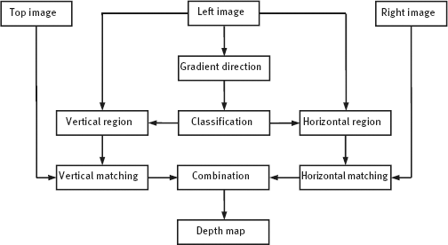
2.5.2.1Algorithm Flowchart

The principle of this method is first to compare the smoothness of regions along the horizontal direction and the vertical direction. In horizontal smoother regions, the matching is based on a vertical image pair. In vertical smoother regions, the matching is based on the horizontal image pair. To judge whether a region is horizontal smooth or vertical smooth, the gradient direction of this region is used. The flowchart of this algorithm is shown in Figure 2.15.

The algorithm has four steps.

(1)Compute the gradients of fL(x, y) and obtain the gradient direction of each point in fL(x, y).

(2)Classify fL(x, y) into two parts with near horizontal gradient directions and near vertical gradient directions, respectively.

(3)Use the horizontal pair of images to compute the disparity in near horizontal gradient direction regions, and use the vertical pair of images to compute the disparity in near vertical gradient direction regions.

(4)Combine the disparity values of the above two results to form a complete disparity image and then a depth image.

In gradient image computation, only two gradient directions are required. A simple method is to select the horizontal gradient value Gh and the vertical gradient value Gv as (W represents the width of the mask for gradient computation)

$G_{\text{h}}\left(x,y\right)={\displaystyle \sum _{i=1}^{W/2}{\displaystyle \sum _{j=y-W/2}^{y+W/2}\left|f_L\left(x-i,j\right)-f_L\left(x+i,j\right)\right|}}\left(2.46\right)$

$G_{\text{v}}\left(x,y\right)={\displaystyle \sum _{i=1}^{W/2}{\displaystyle \sum _{j=x-W/2}^{x+W/2}\left|f_L\left(x-y,j\right)-f_L\left(x,y+j\right)\right|}}\left(2.47\right)$

The following classification rules can be used. If Gh > Gv at a pixel in fL(x, y), this pixel should be classified to the part with near horizontal gradient directions and be searched in the horizontal image pair. If Gh < Gv at a pixel in fL(x, y), this pixel should be classified as the part with near vertical gradient directions and be searched in the vertical image pair.

Example 2.5 A real example in reducing the mismatching caused by smooth regions with orthogonal trinocular matching.

A real example in reducing the influence of smooth regions on stereo matching in Example 2.1 by using the above orthogonal trinocular matching based on the gradient classification is shown in Figure 2.16. Figure 2.16(a) is the top image corresponding to the left and right images in Figure 2.3(a, b), respectively. Figure 2.16(b) is the gradient image of the left image. Figure 2.16(c, d) represents the near horizontal gradient direction image and the near vertical gradient direction image, respectively. Figure 2.16(e, f) represents disparity maps obtained by matching with the horizontal image pair and the vertical image pair, respectively. Figure 2.16(g) is the complete disparity image obtained by combining Figure 2.16(e, f), respectively. Figure 2.16(h) is its corresponding 3-D plot. Comparing Figure 2.16(g) and 2.16(h), with Figure 2.3(c) and 2.3(d), respectively, the mismatching has been greatly reduced with the orthogonal trinocular matching.

2.5.2.2Some Discussions on Mask Size

Two types of masks have been used in the above procedure. One is the gradient mask used to compute the gradient-direction, another is the matching (searching) mask used to compute the correlation between gray-level regions. The sizes of both gradient masks and matching masks influence the matching performance, Jia (1998).

The influence of gradient masks can be explained with the help of Figure 2.17, in which two regions (with vertices A, B, C, and with vertices B, C, D, E) of different gray levels are given. Suppose that the point that needs to be matched is P, which is located near the horizontal edge segment BC. If the gradient mask is too small, as is the case of the square in Figure 2.17(a), the horizontal and vertical regions are hardly separated as Gh ≈ Gv. It is thus possible that the matching at P will be carried out with the horizontal image pair, for instance, and the mismatching could occur due to the smoothness in the horizontal direction. On the other hand, if the gradient mask is big enough, as is the case of the square in Figure 2.17(b), the vertical image pair will be selected and used for the matching at P, and the error matching will be avoided.

The size of the matching mask also has great influence on the performance of the matching. Big masks can contain enough variation for matching to reduce the mismatching, but big masks can also produce big smoothness. The following two cases should be distinguished.

(1)Matching is around the boundary of texture regions and smooth regions, as shown in Figure 2.18(a). If the mask is small and can only cover smooth regions, the matching will have some randomness. If the mask is big and covers both two types of regions, correct matching can be achieved by selecting suitable matching images.

(2)Matching is around the boundary of two texture regions, as shown in Figure 2.18(b). As the mask is always inside the texture regions, the correct matching can be achieved no matter what the size of the mask is.

Example 2.6 Results of orthogonal matching of multiple imaging.

In addition to orthogonal trinocular images, one more image along the horizontal direction and one more image along the vertical direction are used (i. e., multiple imaging along both direction) to give the disparity map shown in Figure 2.19(a). Figure 2.19(b) is its 3-D plot. The results here are even better than those shown in Figure 2.16.

2.6Computing Subpixel-Level Disparity

In a number of cases, pixel-level disparity obtained by normal stereo-matching algorithms is not precise enough for certain measurements. The computation of the subpixel-level disparity is thus needed. In the following, an adaptive algorithm based on local variation patterns of the image intensity and disparity is introduced, which could provide subpixel-level precision of the disparity, Kanade (1994).

Consider a statistical distribution model for first-order partial differential of the image intensity and disparity used for stereo matching, Okutomi (1992). Suppose that images fL(x, y) and fR(x, y) are the left and right images of an intensity function f(x, y), respectively. The correct disparity function between fL(x, y) and fR(x, y) is dr(x, y), which is expressed by

$f_R\left(x,y\right)=f_L\left[x+d_{\text{r}}\left(x,y\right),y\right]+n_{\text{L}}\left(x,y\right)\left(2.48\right)$

where nL(x, y) is the Gaussian noise satisfying $N(0,{\sigma }_n^2).$ Suppose that two matching windows WL and WR are placed at the correct matching position in the left and right images, respectively. In other words, WR is placed at pixel (0, 0) in the right image fR(x, y), while WL is placed at pixel [dr(0,0), 0] in the left image fL(x, y). If the disparity values in the matching windows are constants, that is, dr(u, v) = dr(0,0), fR(u, v) should be equal to fL[u + dr(0,0), v] if no noise influence exists. In real situations, dr(u, v) in the matching window is a variable. Expanding fL[u + dr(u, v), v] at dr(0,0) gives

$\begin{array}{l}{f}_{\text{L}}\left[u+d_{\text{r}}\left(u,v\right),v\right]\approx f_{\text{L}}\left[u+d_{\text{r}}\left(0,0\right),v\right]\left(2.49\right)\\ +\left[d_{\text{r}}\left(u,v\right)-d_{\text{r}}\left(0,0\right)\right]\frac{\partial }{\partial u}{f}_{\text{L}}\left[u+d_{\text{r}}\left(0,0\right),v\right]+n_L\left(u,v\right)\end{array}$

Substituting eq. (2.49) into eq. (2.48) yields

$\begin{array}{l}{f}_{\text{R}}\left(u,v\right)-f_{\text{L}}\left[u+d_{\text{r}}\left(0,0\right),v\right]\approx \left[d_{\text{r}}\left(u,v\right)-d_{\text{r}}\left(0,0\right)\right]\frac{\partial }{\partial u}{f}_L\left[u+d_{\text{r}}\left(0,0\right),v\right]+n_L\left(u,v\right)\\ \left(2.50\right)\end{array}$

Suppose that the disparity dr(u, v) in the matching windows satisfies the following statistical distribution model, Kanade (1991)

$d_{\text{r}}\left(u,v\right)d_{\text{r}}\left(0,0\right)~N\left(0,k_d\sqrt{u^2+v^2}\right)\left(2.51\right)$