
The real world is 3-D. The purpose of 3-D vision is to recover the 3-D structure and description of a scene and to understand the properties of objects and the meaning of a scene from an image or an image sequence. Stereo vision is an important technique for getting 3-D information. Though the principles of 3-D vision can be considered a mimic of the human vision system, modern stereo vision systems have more variations.
The sections of this chapter are arranged as follows:
Section 2.1 provides an overview of the process of stereoscopic vision by listing the six functional modules of stereo vision.
Section 2.2 describes the principle of binocular stereo matching based on region gray-level correlation and several commonly used techniques.
Section 2.3 introduces the basic steps and methods of binocular stereo matching based on different kinds of feature points, and the principle of obtaining the depth of information from these feature points.
Section 2.4 discusses the basic framework of horizontal multiple stereo matching, which using the inverted distance can, in principle, reduce the mismatch caused by periodic patterns.
Section 2.5 focuses on the method of orthogonal trinocular stereo matching, which can eliminate the mismatch caused by the smooth region of the image through matching both the horizontal direction and the vertical direction at the same time.
Section 2.6 presents an adaptive algorithm that is based on local image intensity variation pattern and local disparity variation pattern to adjust the matching window to obtain the parallax accuracy of subpixel level.
Section 2.7 introduces an algorithm to detect the error in the disparity map obtained by stereo matching and to make corresponding corrections.
A stereo vision system normally consists of six modules, Barnard (1982). In other words, six tasks are needed to perform stereo vision work.
Camera calibration determines the internal and external parameters of a camera, according to certain camera models, in order to establish the correspondence between the real points in the scene and the pixels in the image. In stereo vision, several cameras are often used, each of which needs to be calibrated. When deriving 3-D information from 2-D computer image coordinates, if the camera is fixed, the calibration can be carried out only once; if the camera is moving, several calibrations might be needed.
Image capture or image acquisition deals with both spatial coordinates and image properties, as discussed in Chapter 2 of Volume I of this book set. For stereo imaging, several images are required, and each is captured in a normal way, but the relation among them should also be determined. The commonly used stereo vision systems have two cameras, but recently, even more cameras are used. These cameras can be aligned in a line, but can also be arranged in other ways. Some typical examples have been discussed in Chapter 2 of Volume I of this book set.
Stereo vision uses the disparity between different observations in space to capture 3-D information (especially the depth information). How to match different views and find the correspondence of control points in different images are critical. One group of commonly used techniques is matching different images based on well-selected image features. Feature is a general concept, and it can be any abstract representation and/or a description based on pixels or pixel groups. There is no unique theory for feature selection and feature detection, so feature extraction is a problem-oriented procedure. Commonly used features include, in an ascending order of the scales, point-like features, line-like features, and region-like features. In general, larger-scale features could contain abundant information, based on which fast matching can be achieved with a smaller number of features and less human interference. However, the process used to extract them would be relatively complicated and the location precision would be poor. On the other hand, smaller-scale features are simple to represent or describe and they could be located more accurately. However, they are often required in a large number and they normally contain less information. Strong constraints and suitable strategy are needed for robust matching.
Stereo matching consists of establishing the correspondence between the extracted features, further establishing the relation between pixels in different images, and finally obtaining the corresponding disparity images. Stereo matching is often the most important and difficult task in stereo vision. When a 3-D scene is projected on a 2-D plan, the images of the same object under different viewpoints can be quite different. In addition, as many variance factors, such as lighting condition, noise interference, object shape, distortion, surface property, camera characteristics, and so on, are all mixed into a single gray-level value, determining different factors from the gray levels is a very difficult and challenging problem. This problem, even after many research efforts, has not been well resolved. In the following sections, stereo-matching methods based on region correlation and feature match up will be described.
2.1.5Recovering of 3-D Information
Once disparity images are obtained by stereo matching, the depth image can be calculated and the 3-D information can be recovered. The factors influencing the precision of the distance measurement include quantization effect, camera calibration error, feature detection, matching precision, and so on. The precision of the distance measurement is propositional to the match and location precision, and is propositional to the length of the camera baseline (connecting different positions of cameras). Increasing the length of the baseline can improve the precision of the depth measurement, but at the same time, it could enlarge the difference among images, raise the probability of object occlusion and thus augment the complexity of the matching. To design a precise stereo vision system, different factors should be considered together to keep a high precision for every module.
The 3-D information obtained after the above steps often exhibits certain errors due to variance reasons or factors. These errors can be removed or reduced by further postprocessing. Commonly used post-processes are the following three types.
2.1.6.1Depth Interpolation
The principal objective of stereo vision is to recover the complete information about the visible surface of objects in the scene. Stereo-matching techniques can only recover the disparity at the feature points, as features are often discrete. After the feature-based matching, a reconstruction step for interpolating the surface of the disparity should be followed. This procedure interpolates the discrete data to obtain the disparity values at nonfeature points. There are diverse interpolation methods, such as nearest-neighbor interpolation, bilinear interpolation, spline interpolation, model-based interpolation, and so on, Maitre (1992). During the interpolation process, the most important aspect is to keep the discontinuous information. The interpolation process is a reconstruction process in some sense. It should fit the surface consistence principles, Grimson (1983).
2.1.6.2Error Correction
Stereo matching is performed among images suffering from geometrical distortion and noise interference. In addition, periodical patterns, smoothing regions in the matching process, occluding effects, nonstrictness of restriction, and so on, can induce different errors in disparity maps. Error detection and correction are important components of post-processing. Suitable techniques should be selected according to the concrete reasons for error production.
2.1.6.3Improvement of Precision
Disparity computation and depth information recovery are the foundation of the following tasks. Therefore, high requirements about disparity computation are often encountered. To improve the precision, subpixel-level precision for the disparity is necessary, after obtaining the disparity at the pixel level.
2.2Region-Based Binocular Matching
The most important task needed to obtain the depth images is to determine the correspondence between the related points in binocular images. In the following, the discussion considers parallel horizontal models. By considering the geometrical relations among different models, the results obtained for parallel horizontal models can also be extended to other models (see Section 2.2 of Volume I in this book set).
Region-based matching uses gray-level correlation to determine the correspondence. A typical method is to use the mean-square difference (MSD) to judge the difference between two groups of pixels needed to be matched. The advantage of this method is that the matching results are not influenced by the precision of different feature detections, so high-accuracy locations of the points and a dense disparity surface can be obtained, Kanade (1996). The disadvantage of this method is that it depends on the statistics of gray-level values of images and thus is quite sensitive to the structure of the object surface and the illumination reflection. When the object surfaces lack enough texture detail or if there is large distortion in capturing the image, this matching technique will encounter some problems. Besides gray-level values, other derived values from gray levels, such as the magnitude or direction of gray-level differential, Laplacian of gray level, curvature of gray level, and so on, can also be used in region-based matching. However, some experiments have shown that the results obtained with gray-level values are better than the results obtained with other derived values, Lew (1994).
Template matching can be considered the basis for region-based matching. The principle is to use a small image (template) to match a subregion in a big image. The result of such a match is used to help verify if the small image is inside the big image, and locate the small image in the big image if the answer is yes. Suppose that the task is to find the matching location of a J × K template w(x, y) in an M × N image f (x, y). Assume that J ≤ M and K ≤ N. In the simplest case, the correlation function between f (x, y) and w(x, y) can be written as

where s = 0,1,2,.., M − 1 and t = 0, 1, 2,..., N − 1. The summation in eq. (2.1) is for the overlapping region of f(x, y) and w(x, y). Figure 2.1 illustrates the situation, in which the origin of f(x, y) is at the top-left of image and the origin of w(x, y) is at its center. For any given place (s, t) in f(x, y), a particular value of c(s, t) will be obtained. With the change of s and t, w(x, y) moves inside f(x, y). The maximum of c(s, t) indicates the best matching place.
Besides the maximum correlation criterion, another criterion used is the minimum mean error function, given by
In VLSI hardware, the calculation of square operation is complicated. Therefore, the square value is replaced by an absolute value, which gives a minimum average difference function,
The correlation function given in eq. (2.1) has the disadvantage of being sensitive to changes in the amplitude of f(x, y) and w(x, y). To overcome this problem, the following correlation coefficient can be defined, given by
where s = 0, 1, 2,..., M − 1, t = 0, 1, 2, ..., N − 1, is the average value of w(x, y), and (x, y) is the average value of f(x, y) in the region coincident with the current location of w(x, y). The summations are taken over the coordinates that are common to both f(x, y) and w(x, y). Since the correlation coefficient C(s, t) is scaled in the interval [−1, 1], its values are independent to the changes in the amplitude of f(x, y) and w(x, y).
Following the principle of template matching, a pair of two stereo images (called left and right images) can be matched. The process consists of four steps:
(1)Take a window centered at a pixel in the left image.
(2)Construct a template according to the gray-level distribution in the above window.
(3)Use the above template to search around all pixels in the right image in order to find a matching window.
(4)The center pixel in this matching window is the pixel corresponding to the pixel in the left image.
2.2.2.1Constraints
A number of constraints can be used to reduce the computational complexity of stereo matching. The following list gives some examples, Forsyth (2003).
Compatibility Constraint The two matching pixels/regions of two images must have the same physical properties, respectively.
Uniqueness Constraint The matching between two images is a one-to-one matching.
Continuity Constraint The disparity variation near the matching position should be smooth, except at regions with occlusion.
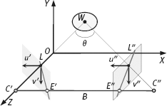
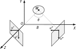
Epipolar Line Constraint Look at Figure 2.2. The optical center of the left camera is located at the origin of the coordinate system, the two optical centers of the left and right cameras are connected by the X-axis, and their distance is denoted B (also called the baseline). The optical axes of the left and right image planes lie in the XZ plane with an angle (between them. The centers of the left and right image planes are denoted C′ and C″, respectively. Their connecting line is called the optical centerline. The optical centerline crosses the left and right image planes at points E′ and E″, respectively. These two points are called epipoles of the left and right image planes, respectively. The optical centerline is in the same plane as the object point W. This plane is called the epipolar plane, which crosses the left and right image planes at lines L′ and L″. These two lines are called the epipolar lines of object point W projected on the left and right image planes. Epipolar lines limit the corresponding points on two stereo images. The projected point of object point W on the right image plane, corresponding to the left image plane, must lie on L″. On the other hand, the projected point of object point W on the left image plane, corresponding to the right image plane, must lie on L′.
2.2.2.2Factors Influencing View Matching
Two important factors influencing the matching between two views are:
(1)In real applications, due to the shape of objects or the occlusion of objects, not all objects viewed by the left camera can be viewed by the right one. In such cases, the template determined by the left image may not find any matching place in the right image. Some interpolation should be performed to estimate the matching results.
(2)When the pattern of a template is used to represent the pixel property, the assumption is that different templates should have different patterns. However, there are always some smooth regions in an image. The templates obtained from these smooth regions will have the same or similar patterns. This will cause some uncertainty that will induce some error in the matching. To solve this problem, some random textures can be projected onto object surfaces. This will transform smooth regions to textured regions so as to differentiate different templates.
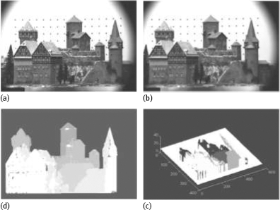
Example 2.1 Real examples of the influence of smooth regions on stereo matching. Figure 2.3 gives a set of examples showing the influence of smooth regions on stereo matching. Figure 2.3(a, b) represents the left and right images of a pair of stereo images, respectively. Figure 2.3(c) is the disparity map obtained with stereo vision, in which darker regions correspond to small disparities and lighter regions correspond to large disparities. Figure 2.3(d) is the 3-D projection map corresponding to Figure 2.3(c). Since some parts of the scene, such as the horizontal eaves of the tower and the building, have similar gray-level values along the horizontal direction, the search along it will produce errors due to mismatching. These errors are manifested in Figure 2.3(c) by the nonharmonizing of certain regions with respect to surrounding regions and are visible in Figure 2.3(d) by some sharp burrs.
![]()
2.3Feature-Based Binocular Matching
One method to determine the correspondence between the related parts in binocular images is to select certain feature points in images that have a unique property, such as corner points, inflexion points, edge points, and boundary points. These points are also called the control points or the matching points.
The main steps involved in a feature-based matching are listed in the following:
(1)Select several pairs of control points from binocular images.
(2)Match these pairs of points (see below).
(3)Compute the disparity of the matched points in two images to obtain the depth at the matching points.
(4)Interpolate sparse depth values to get a dense depth map.
Some basic methods for feature-based matching are presented first.
2.3.1.1Matching with Edge Points
A simple method for matching uses just the edge points, Barnard (1980). For an image f(x, y), its edge image can be defined as
where H (horizontal), V (vertical), L (left), and R (right) are defined by
Decompose t(x, y) into small nonoverlap regions W, and take the points with the maximum value in each region as the feature points. For every feature point in the left image, consider all possible matching points in the right image as a set of points. Thus, a label set for every feature point in the left image can be obtained, in which label l can be either the disparity of a possible matching or a special label for nonmatching. For every possible matching point, the following computation is performed to determine the initial matching probability P(0)(l)
where l = (lx, ly) is the possible disparity and A(l) represents the gray-level similarity between two regions and is inversely proportional to P(0)(l). Starting from P(0)(l), assigning positive increments to the points with small disparities and negative increments to the points with large disparities can update P(0)(l) with a relaxation method. With the iteration, the kth matching probability P(k)(l) for correct matching points will increase and that for incorrect matching points will decrease. After certain iterations, the points with maximum P(k)(l) can be determined as matching points.
2.3.1.2Matching with Zero-Crossing Points
Using the convolution with the Laplacian operator can produce zero-crossing points. The patterns around zero-crossing points can be taken as matching elements, Kim (1987). Consider the different connectivity of zero-cross points. Sixteen zero-cross patterns can be defined as the shades shown in Figure 2.4.
For each zero-cross pattern in the left image, collect all possible matching points in the right image to form a set of possible matching points. In stereo matching, assign an initial matching probability to each point. Using a similar procedure as for matching with edge points, the matching points can be found by iterative relaxation.
2.3.1.3Depth of Feature Points
In the following, Figure 2.5 (obtained by removing the epipolar lines in Figure 2.2 and moving the baseline to the X-axis) is used to explain the corresponding relations among feature points.

In a 3-D space, a feature point W(x, y, −z), after respective projections on the left and right images, will be
In eq. (2.12), the computation for u" is made by two coordinate transformations: A translation followed by a rotation. Equation (2.12) can also be derived with the help of Figure 2.6, which shows a plane that is parallel to the XZ plane in Figure 2.5. This is given by
By noting that W is on the −Z axis, it is easy to get
Once u″ is determined from u′ (i. e., the matching between feature points is established), the depth of a point that is projected on u′ and u″ can be determined from eq. (2.13) by

2.3.1.4Sparse Matching Points
Feature points are particular points on the objects and they are located apart from each other. The dense disparity map cannot be obtained only from the sparse matching points, so it is impossible to recover uniquely the object shape. For example, four points of a co-plane are shown in Figure 2.7(a), which are the sparse matching points obtained by the disparity computation. Suppose that these points are on the surface of an object, then it is possible to find an infinite number of surfaces that pass these four points. Figure 2.7(b–d) is just a few of them. It is evident that it is not possible to recover uniquely the object shape from the sparse matching points.
2.3.2Matching Based on Dynamic Programming
Matching of feature points is needed to establish the corresponding relations among feature points. This task can be accomplished with the help of ordering constraints (see below) and by using dynamic programming techniques, Forsyth (2003).
The ordering constraint is also a popularly used type of constraint in stereo matching, especially for feature-based matching. Consider three feature points on the surface of an object in Figure 2.8(a). They are denoted sequentially by A, B, and C. The orders of their projections on two images are just reversed as c, b, a, and c′, b′, a′, respectively. This inverse of the order of the corresponding points is called the ordering constraint. In real situations, this constraint may not always be satisfied. For example, when a small object is located in front of a big object as shown in Figure 2.8(b), the small object will occlude parts of the big object. This does not only removes points c and a′ from the resulted images, but also violates the ordering constraint for the order of the projections on images.
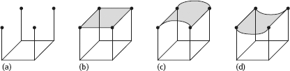
Figure 2.7: It is not possible to recover uniquely the object shape from the sparse matching points.

However, in many cases, the ordering constraint is still held, and can be used to design stereo-matching techniques based on dynamic programming (see Section 2.2.2 in Volume II of this book set). The following discussion assumes that a set of feature points has been found on corresponding epipolar lines, as shown in Figure 2.8. The objective is to match the intervals separating those points along the two intensity profiles, as shown in Figure 2.9(a). According to the ordering constraint, the order of the feature points must be the same, although the occasional interval in either image may be reduced to a single point corresponding to the missing correspondences associated with the occlusion and/or noise.
The above objective can be achieved by considering the problem of matching feature points as a problem of optimization of a path’s cost over a graph. In this graph, nodes correspond to pairs of the left and right feature points and arcs represent matches between the left and right intervals of the intensity profile, bounded by the features of the corresponding nodes, as shown in Figure 2.9(b). The cost of an arc measures the discrepancy between the corresponding intervals.
2.4Horizontal Multiple Stereo Matching
In horizontal binocular stereo vision, there is the following relation between the disparity d of two images and the baseline B linking two cameras (λ represents focal length)
The last step is made in considering that the distance Z λ is satisfied in most cases. From eq. (2.16), the disparity d is proportional to the baseline length B, for a given distance Z. The longer the baseline length B is, the more accurate the distance computation is. However, if the baseline’s length is too long, the task of searching the matching points needs to be accomplished in a large disparity range. This not only increases the computation but also causes mismatching when there are periodic features in the image (see below).
One solution for the above problem is to use a control strategy of matching from coarse to fine scale, Grimson (1985). That is, start matching from low-resolution images to reduce the mismatching and then progressively search in high-resolution images to increase the accuracy of the measurement.
2.4.1Horizontal Multiple Imaging
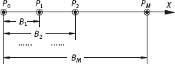
Using multiple images can solve the above problem to improve the accuracy of the disparity measurement, Okutomi (1993). In this method, a sequence of images (along the horizontal direction) are used for stereo matching. The principle is to reduce the mismatching error by computing the sum of the squared difference (SSD), Matthies (1989). Suppose that a camera is moving horizontally and captures a set of images fi(x, y), i = 0, 1,..., M at locations P0, P1, P2,..., PM, with baselines B1, B2,..., BM, as shown in Figure 2.10.
According to Figure 2.10, the disparity between two images captured at points P0 and Pi, respectively, is
As only the horizontal direction is considered, f(x, y) can be replaced by f(x). The image obtained at each location is
where noise ni(x) is assumed to have a Gaussian distribution with a mean of 0 and a variance of
The value of SSD at x in f0(x) is
where W represents the matching window and is the estimated disparity value at x. Since SSD is a random variable, its expected value is
where Nw denotes the number of pixels in the matching windows. Equation (2.20) indicates that Sd(x; ![]() ) attains its minimum at di =
) attains its minimum at di = ![]() . If the image has the same gray-level patterns at x and x + p(p ≠ 0), it has
. If the image has the same gray-level patterns at x and x + p(p ≠ 0), it has
From eq. (2.20), it will have
Equation (2.22) indicates that the expected values of SSD will attain extremes at two locations x and x + p. In other words, there is an uncertainty problem or ambiguity problem, which will produce a mismatching error. Such a problem has no relation with the length or the number of baselines, so the error cannot be avoided even with multiple images.
The inverse-distance t is defined as
From eq. (2.16),
where ti and are the real and estimated inverse-distances, respectively. Taking eq. (2.25) into eq. (2.19), the SSD corresponding to t is
Its expected value is
Taking the sum of SSD for M inverse-distance gives SSSD (sum of SSD) in inverse-distance
The expected value of this new measuring function is