Synchronous, permanent magnet and reluctance motors and drives
Abstract
This increasingly important group of motors (that includes the so-called ‘brushless d.c.’) have the potential to eclipse the induction motor in terms of efficiency because, like the d.c. machine, the ‘excitation’ or flux-producing mechanism is separate from the work producing part. We cover fixed-frequency and inverter-fed operation of excited rotor, permanent magnet, reluctance, and salient PM. For each type we also discuss the field orientation techniques that not only provide high dynamic performance but also ensure self-synchronisation, thereby eliminating the danger of stalling.
Keywords
Synchronous motors; Permanent magnet (PM); Salient; Field oriented control; Field weakening; Reluctance motor; Reluctance torque; Performance
9.1 Introduction
Chapters 6–8 have described the virtues of the induction motor and how, when combined with power electronic control, it is capable of meeting the performance and efficiency requirements of many of the most demanding applications. In this chapter another group of a.c. motors is described. In all of them the electrical power that is converted to mechanical power is fed into the stator, so, as with the cage induction motor, there are no sliding contacts in the main power circuits. The majority have stators that are identical (or very similar) to the induction motor, but some new constructional and winding techniques involving segmented construction are being applied at the lower power end: these will be introduced later.
It has to be admitted that the industrial and academic communities have served to make life confusing in this area by giving an array of different names to essentially the same machine, so we begin by looking at the terminology. The names we will encounter include:
- (a) Conventional Synchronous Machine with its rotor field winding (excited-rotor). This is the only machine that may have brushes, but even then they will only carry the rotor excitation current, not the main a.c. power input.
- (b) Permanent Magnet Synchronous Machine with permanent magnets replacing the rotor field winding.
- (c) Brushless Permanent Magnet Synchronous Motor (same as (b)). The prefix ‘brushless’ is superfluous.
- (d) Brushless a.c. Motor (same as (b).
- (e) Brushless d.c. Motor (same as (b) except for detailed differences in the field patterns). This name was coined in the 1970s to describe ‘inside out’ motors that were intended as direct replacements for conventional d.c. motors, and in this sense it has some justification.
- (f) Permanent Magnet Servo Motor (same as (b)).
The Reluctance motor is fundamentally different from all the above types. Whilst it rotates at synchronous speed, it does not have any form of excitation on the rotor and the method of torque production is somewhat different. It is nonetheless an increasingly important type of electrical machine.
Traditionally, as their name implies, synchronous motors were designed for operation directly off the utility supply, usually at either 50 Hz or 60 Hz. They then operate at a specific and constant speed (determined by the pole-number of the winding) over a wide range of loads, and therefore can be used in preference to induction motors when precise (within the tolerance of the utility frequency) constant speed operation is essential: there is no load-dependent slip as is unavoidable with the induction motor. These machines are available over a very wide range from tiny single-phase versions in domestic clocks and timers to multi-megawatt machines in large industrial applications such as gas compressors. (The clock application means that utility companies have a responsibility to ensure that the average frequency over a 24 h period always has to be precisely the rated frequency of the supply in order to keep us all on time. Ironically, in order to do this, they control the speed of very large, turbine-driven, synchronous machines that generate the vast majority of the electrical power throughout the world.)
To overcome the fixed-speed limitation that results from the constant frequency of the utility supply, inverter-fed synchronous motor drives are widely used. We will see that all forms of this generic technology use a variable-frequency inverter to provide for variation of the synchronous speed, but that in almost all cases, the switching pattern of the inverter (and hence the frequency) is determined by the rotor position and not by an external oscillator. In such so called ‘self-synchronous’ drives, the rotor is incapable of losing synchronism and stalling (which is one of the main drawbacks of the utility-fed machine). Field oriented control can be applied to synchronous machines to achieve the highest levels of performance and efficiency with machines which have higher inherent power densities than the equivalent induction motors.
9.2 Synchronous motor types
In the synchronous motor, the stator windings are essentially the same as in the induction motor, so when connected to the 3-phase supply, a rotating magnetic field is produced. However, instead of having a cylindrical rotor with a cage winding which automatically adapts to the pole number of the stator field, the synchronous motor has a rotor with either a d.c. excited winding (supplied via sliprings, or on larger machines an auxiliary exciter1), or permanent magnets, designed with the same pole number as the stator. The rotor is thus able to ‘lock-on’ or ‘synchronise with’ the rotating magnetic field produced by the stator. Once the rotor is synchronised, it will run at exactly the same speed as the rotating field despite load variation, so under constant-frequency operation the speed will remain constant as long as the supply frequency is stable.
As previously shown, the synchronous speed (in rev/min) is given by the expression

where f is the supply frequency and p is the pole-number of the winding. Hence for 2, 4 and 6-pole industrial motors the running speeds on a 50 Hz supply are 3000, 1500, and 1000 rev/min, while on a 60 Hz supply they become 3600, 1800, and 1200 rev/min respectively. At the other extreme, the little motor in a time switch with its cup-shaped rotor with 20 axially projecting fingers and a circular coil in the middle is a 20-pole reluctance (synchronous) motor that will run at 300 rev/min when fed from a 50 Hz supply. Users who want speeds different from these discrete values will be disappointed, unless they are prepared to invest in a variable-frequency inverter.
With the synchronous machine, we find that there is a limit to the maximum (pull-out) torque (see Section 9.3) which can be developed before the rotor is forced out of synchronism with the rotating field. This ‘pull-out’ torque will typically be 1.5 times the continuous rated torque but can be designed to be as high as 4 or even 6 times higher in the case of high performance PM motors where, for example, high accelerating torques are needed for relatively short periods. For all torques below pull-out the steady running speed will be absolutely constant. The torque-speed curve is therefore simply a vertical line at the synchronous speed, as shown in Fig. 9.1. We can see that the vertical line extends into quadrant 2, which indicates that if we try to force the speed above the synchronous speed the machine will act as a generator.

Traditionally, utility-fed synchronous motors were used where a constant speed is required, high efficiency desirable, and power factor controllable. They were also used in some applications where a number of motors were required to run at precisely the same speed. However, a group of utility-fed synchronous motors could not always replace mechanical shafting2 because whilst their rotational speed would always be matched, the precise relative rotor angle of each motor would vary depending on the load on the individual motor shafts.
9.2.1 Excited-rotor motors
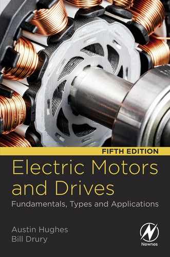
The rotor of a conventional synchronous machine carries a ‘field’ or ‘excitation’ winding which is supplied with direct current either via a pair of sliprings on the shaft, or via an auxiliary brushless exciter on the same shaft. The field winding is designed to produce an air-gap field of the same pole-number and spatial distribution (usually sinusoidal) as that produced by the stator winding. The rotor may be more-or-less cylindrical, with the field winding distributed in slots (Fig. 9.2A), or it may have projecting (‘salient’) poles around which the winding is concentrated (Fig. 9.2B).
A cylindrical-rotor motor has little or no reluctance (self-aligning) torque (discussed later), so it can only produce torque when current is fed into the rotor. On the other hand, the salient-pole type also produces some reluctance torque even when the rotor winding has no current. In both cases, however, the rotor ‘excitation’ power is relatively small, since all the mechanical output power is supplied from the stator side.
Excited rotor motors are used in sizes ranging from a few kW up to many MW. The large ones are effectively alternators (as used for power generation) but used as motors. Wound rotor induction motors (see Chapter 6) can also be made to operate synchronously by supplying the rotor with d.c. through the sliprings.
As we will see later, an advantage of the excited rotor type is that the power factor can be controlled over a wide range by varying the rotor excitation current.
9.2.2 Permanent magnet motors
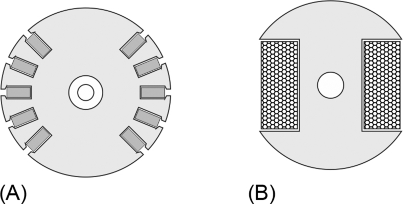
The synchronous machines considered so far require two electrical supplies, the first to feed the field/excitation and the second to supply the stator. Brushless permanent magnet (Brushless PM) machines have magnets attached to the rotor to provide the field, and so only a stator supply is required. The principle is illustrated for 4-pole surface-mounted and 10-pole buried/interior types in Fig. 9.3. Motors of this sort have typical output ranging from about 100 W up to perhaps 500 kW, though substantially higher ratings have been made.
The advantages of the permanent magnet type are that no supply is needed for the rotor and the rotor construction can be robust and reliable. The disadvantage is that the excitation is inherently fixed, so the designer must either choose the shape and disposition of the magnets to match the requirements of one specific load, or seek a general-purpose compromise. Control of power-factor via excitation is of course no longer possible. Within these constraints the Brushless PM synchronous motor behaves in very much the same way as its excited-rotor sister.
9.2.3 Reluctance motors
The reluctance motor is arguably the simplest synchronous motor of all, the rotor consisting simply of a set of laminations shaped so that it tends to align itself with the field produced by the stator. This ‘reluctance torque’ action is discussed in Section 9.3.3.
Until recently reluctance motors were intended for use from the utility supply, so in order to get the rotor up to a speed close enough to the synchronous speed for the rotor to make the final leap and lock onto the rotating stator field, the rotor also carries a cage winding which provides accelerating torque for the run-up, but thereafter carries no current. The rotor therefore resembles a cage induction motor, with parts of the periphery cut away in order to force the flux from the stator to enter the rotor in the remaining regions where the air-gap is small, as shown in Fig. 9.4A. Alternatively, the ‘preferred flux paths’ can be imposed by removing iron inside the rotor so that the flux is guided along the desired path, as shown in Fig. 9.4B and C, the latter being for an inverter-fed motor, where a starting cage is not required. All these rotor types can be seen to have “salient” poles.

The rotor will tend to align itself with the field, and hence is able to remain synchronised with the travelling field set up by the 3-phase winding on the stator in much the same way as a permanent-magnet rotor. Early reluctance motors were invariably one or two frame sizes bigger than an induction motor for a given power and speed, and had low power-factor and poor pull-in performance. As a result they fell from favour except for some special applications such as textile machinery where large numbers of cheap synchronised motors driven from a single variable frequency inverter were used. Understanding of reluctance motors is now much more advanced, though their fundamental performance still lags the induction motor as regards power-output, power factor and efficiency. Recently, there is renewed interest in rotors that exploit both permanent magnet and reluctance torque, and this is discussed in Section 9.3.5.
9.2.4 Hysteresis motors
Whereas most motors can be readily identified by inspection when they are dismantled, the hysteresis motor is likely to baffle anyone who has not come across it before. The rotor consists simply of a thin-walled cylinder of what looks like steel, while the stator has a conventional single-phase or three-phase winding. Evidence of very weak magnetism may just be detectable on the rotor, but there is no hint of any hidden magnets as such, and certainly no sign of a cage. Yet the motor runs up to speed very sweetly and settles at exactly synchronous speed with no sign of a sudden transition from induction to synchronous operation.
These motors (the operation of which is quite complex) rely mainly on the special properties of the rotor sleeve, which is made from a hard steel which exhibits pronounced magnetic hysteresis. Normally in machines we aim to minimise hysteresis in the magnetic materials, but in these motors the effect (which arises from the fact that the magnetic flux density B depends on the previous ‘history’ of the m.m.f.) is deliberately accentuated to produce torque. There is actually also some induction motor action during the run-up phase, and the net result is that the torque remains roughly constant at all speeds.
Small hysteresis motors were once used extensively in office equipment, fans, etc. The near constant torque during run-up and the very modest starting current (of perhaps 1.5 times rated current) means that they are also suited to high inertia loads such as gyro compasses and small centrifuges.
Hysteresis motors are used in niche areas, and so we will not consider them any further.
9.3 Torque production
The aim of this section is to present physical pictures of the torque production mechanism in the various types of synchronous motor. We deliberately concentrate on the same ‘BIl’ approach that we have followed in relation to the d.c. and the induction motor, in order to highlight the fundamental similarities between the three types of motor.
We start with the excited-rotor motor in order to establish a general approach to the interaction between stator and rotor currents and fields, and to develop qualitative expressions for torque. A relatively simple adaptation is then made to deal with the permanent-magnet type, and with a further twist, we can throw light on the torque in a reluctance motor (which has neither winding nor magnets on the rotor). Finally we look briefly at salient pole synchronous motors, which develop both excitation torque and reluctance torque.
The spatial images developed in this section will help later in the chapter when we link them to the voltages and currents in the steady-state time phasor diagram. Readers who are familiar with the theory of electrical machines will be aware that books often omit the material in this section in favour of the coupled-circuit approach that we discussed briefly in Section 8.3; however, we believe that the physical approach will be preferred by our target readership.
9.3.1 Excited rotor motor
In explaining the mechanism of torque production in the induction motor (Chapter 5) we chose to focus on the ‘BIl’ force (and hence the torque) resulting from the interaction between the rotor current wave and the resultant radial flux density wave (i.e. the resultant flux due to the combined effect of the stator and rotor m.m.f.'s), both of which are sinusoidally distributed in space.
For the synchronous machine we could use the same approach for the excited rotor type, but the PM rotor and reluctance versions don't have current on the rotor when running synchronously, so we consider the torque on the stator instead. We assume here that the reader is happy to accept that electromagnetic torque on the rotor will always be accompanied by an equal and opposite torque on the stator.
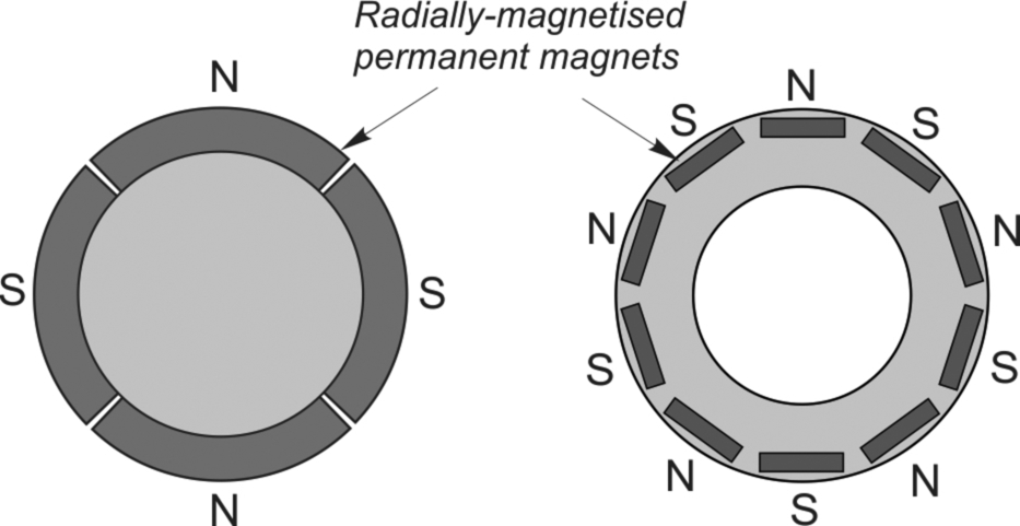
We will explore the torque mechanism by looking first at the static condition (which is equivalent to taking a snapshot of the running condition), as shown in Fig. 9.5. This represents a model of a smooth rotor machine with sinusoidally distributed currents on both stator and rotor: the stator current is fixed in all five sketches, and the rotor current is fixed relative to the rotor. The blue flux lines represent in simplified form the sinusoidal m.m.f. and flux density produced by the rotor current, and so when the rotor turns, they follow; only a few lines are shown for the sake of clarity. The drum on the rotor carries a rope to which weights can be attached to apply mechanical torque to the rotor.
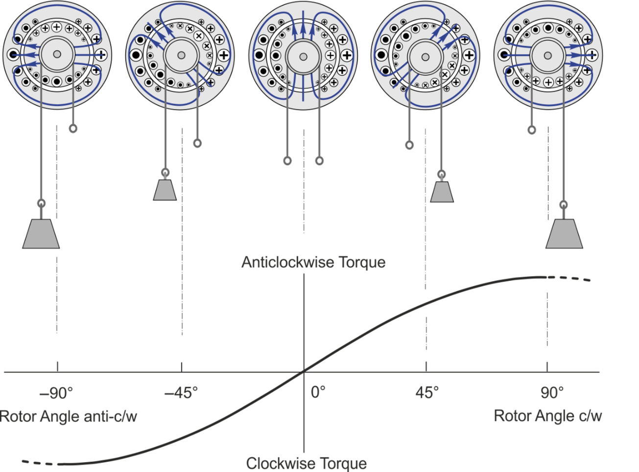
The ‘rule of thumb' relating to the torque produced by the interaction of rotor and stator fields is that the torque always acts so as to move the two fields into alignment. The flux pattern produced by the stator winding is not shown in Fig. 9.5 in order to avoid overcrowding, but it would be similar to the rotor flux, and in all three sketches it would be directed upwards.
Hence if the rotor is free to move, and there is no external torque applied, it will come to rest as shown in the centre sketch, with zero torque. We can confirm that the resultant torque is zero in this position by considering the ‘BIl’ forces on the stator conductors caused by interaction with the rotor flux. Because of the symmetry there is no resultant force on the group of stator conductors carrying positive current, because any in the upper half exposed to positive (outward) flux will experience a clockwise force, while those in the lower half will be exposed to negative (inward) flux, and therefore will experience an equal anticlockwise force. By the same token, there is no resultant force on the conductors carrying negative current, and there is therefore no torque on the stator, and hence none on the rotor.
However, when the rotor is turned in a clockwise direction by a load, as in the two right-hand sketches, more stator conductors carrying positive current are exposed to positive rotor flux, and those carrying negative current are exposed to negative flux. Application of Fleming's left hand rule shows that there is a clockwise torque on the stator, and therefore an equal anti-clockwise torque on the rotor, the torque increasing with angle. When the rotor torque equals the load torque, the rotor is at rest, in a stable equilibrium: If it is displaced in either direction, and then released, it will settle back at the same angle.
The unloaded case shown in the centre sketch is also a stable equilibrium, with any clockwise displacement leading to an anti-clockwise restoring torque, and vice-versa. Beyond 90°, however, the rotor is unstable, and so although there is theoretically another zero torque at 180°, the unloaded rotor could not remain at rest there because the slightest nudge would cause it to flip round in the direction it had been disturbed, and come to rest as in the centre sketch.
The right hand sketch shows the position of maximum torque, the rotor flux being horizontal and aligned with the stator current distribution. Recalling that the flux produced by the stator current is vertical, we see that the condition for maximum torque is that the two fields are perpendicular.
The theoretical torque-angle curve is shown below the three sketches in Fig. 9.5, and is a sinusoidal function of rotor angle. The beginnings of the unstable regions are indicated by dotted lines. The peak torque is, as expected, proportional to the product of the stator current and the rotor current (or flux). For obvious reasons, the angle between the rotor and stator fields is known as the torque angle.
We have considered the stator current to be constant in order to explore the mechanism of torque production, and the mental picture of the two fields always tending to align themselves is a useful one, which we can easily extend to the running condition. We now imagine that the rotor is running in the steady-state at the synchronous speed, with the amplitude and frequency of the stator current kept constant, the rotor being ‘locked onto’ or dragged along by the rotating stator field. The variation of the ‘torque angle’ with load on the shaft is then the same as we have seen in the static case, the angle increasing as the load torque increases. Clearly, if the load torque exceeds the point at which the torque angle is 90°, the rotor will lose synchronism and stall. However it is important to stress that in practice ‘constant stator current’ is not a normal operating condition. When the motor is operated from the utility supply, for example, it is the stator voltage (and frequency) that are constant, while in an inverter-fed drive with field-oriented control (see later), the system will always control the magnitude, speed and instantaneous position of the stator current distribution relative to the rotor position in order to provide the torque required.
Torque—Excited rotor motor
Hitherto, when we have invoked the ‘BIl’ picture to explain the production of torque we have always taken the B to be the resultant flux density, resulting from the combined effect of both stator and rotor currents, but in the discussion above we only considered the torque produced on the stator by the rotor flux. We will now see that if the windings are sinusoidally distributed, and the rotor surface is smooth (i.e. it may have slots, but no major saliencies), there are several ways of expressing the torque, not all involving the resultant flux, and we can choose which suits best according to the circumstances.
We saw in Section 8.2.1 that sinusoidally space-distributed quantities can be represent by space phasors or vectors, so we can represent an m.m.f. (or its corresponding flux density distribution) by a vector whose length is proportional to the m.m.f. (and hence to the current), and whose direction is determined by the instantaneous angular position of the current wave.
The general case is shown in Fig. 9.6, where FS, FR, and F are the stator, rotor and resultant m.m.f.'s respectively. The angle between stator and rotor m.m.f's (the torque angle), is λ, and the angle between the rotor m.m.f. and the resultant m.m.f. (δ) is the load angle (see later). The rotor m.m.f. in this space phasor diagram has been chosen deliberately to be horizontal in order to be consistent with the time phasor diagrams of pm motors that we will discuss later in this chapter.

We have already established that the torque is proportional to the product of the stator and rotor m.m.f.'s, and to the sine of λ, i.e.
The expression FSFR sin λ is the area of the triangle defined by the sides FS and FR, so we see that the area provides an immediate visual indication of the torque. We can also see that when the stator and rotor m.m.f.'s are aligned, the torque is zero, and when they are perpendicular, we get maximum torque.
Readers who are familiar with vector calculus will recognise the expression for the area of a triangle as the amplitude term of the so-called ‘cross product’ of two vectors (i.e. if the vectors are of magnitudes A and B and the angle between them is γ, their cross product is AB sin γ).
The triangles defined by the sides F and FR, and F and FS, both have the same area as the triangle defined by FS and FR, so the torque can equally well be expressed in two further ways, leading to the three equivalent cross-product formulations shown below:
We have used the first of these in slightly modified form in previous chapters, where instead of resultant m.m.f. we talked of resultant flux density, and instead of rotor m.m.f. we used rotor current distribution, but as both are proportional to their respective m.m.f.'s, and we are not being quantitative, there is no inconsistency. In fact, we will often substitute ‘flux density’ or (for a given machine) ‘flux’ in place of m.m.f. later in this chapter when we are discussing what determines the torque.
In the excited rotor case it turns out that the first version is the simplest way of picturing the torque mechanism when the currents are specified (as in an inverter-fed drive), and in particular it defines what we mean by the torque angle, λ. We should also note what many readers may think is obvious, which is that if the rotor m.m.f. is zero, and the only source of excitation is on the stator, the stator flux will not produce any torque. However, this is only true for smooth rotor machines, and things are different for rotors with salient poles, as we will see later.
When we move on to consider steady-state operation from the utility supply, the second torque formulation will prove more fruitful for our discussions, and we will make use of the load-angle (δ) rather than the torque angle.
It is worth mentioning that an alternative way of looking at a cross product is that it can be obtained by taking the product of the first vector with the component of the second that is perpendicular to the first, and we will make use of this later in this chapter, where we refer to the axis of the rotor flux as the ‘direct axis’ and to the perpendicular component as the ‘quadrature axis’ component.
Physically, we picture maximum torque when stator and rotor m.m.f.'s or fluxes are in quadrature, and zero torque when they are aligned. At other angles, we recognise that it is only the quadrature component of the second vector that contributes to torque.
9.3.2 Permanent magnet motor
The permanent magnet (PM) motor (Fig. 9.3) behaves in a similar way as the excited rotor one, with the obvious exception that the ‘strength’ of the flux produced by the magnet cannot be varied once it has been magnetised.
To avoid going deeply into the properties of permanent-magnets, we can picture the magnet as an m.m.f. source, whose external magnetic circuit comprises three reluctances in series, viz. the ‘iron’ part of the rotor body; the stator iron; and the air-gap between rotor and stator iron. The latter term is dominant in any machine, but it is even more so here because the “airgap” is at least equal to the radial thickness of the magnets, and so is much larger than in the excited rotor version. Despite this, the high magnet m.m.f. produces the required flux density at the stator. There is no variation in the reluctance ‘seen’ by the magnet as the rotor turns, so we can picture a rotor flux wave that remains constant and whose instantaneous position is determined by the rotor angle: in future, we will denote this by the symbol φmag.
Looked at from the stator side we might wonder how the magnet material influences the reluctance seen by the stator m.m.f. Again, we can take a simplified view and, as far as an externally applied field is concerned, we treat the magnet material as if it had the same permeability as air. The stator m.m.f. therefore sees a high reluctance because the effective air-gap is much larger than usual due to the radial depth of the magnets. This means the stator self-inductance is much lower than that of a similar excited rotor motor, which is advantageous as far as rapid current control is concerned.
Torque—Permanent magnet motor
In line with our discussion above, if we denote the stator (or, to use the traditional word ‘armature’) flux wave by φarm and the angle between the magnet and stator flux waves (the torque angle) by λ, the torque is expressed by
i.e. the torque depends on product of the rotor and stator fluxes and the sine of the angle between them. Note that we could equally have chosen to use the respective m.m.f.'s in the torque expression rather than the fluxes, in which case the torque expression would be identical to that for the excited rotor case.
9.3.3 Reluctance motor
The reader who absorbed Chapter 1 will recall that the word reluctance is used in the context of magnetic circuits to define the analogous quantity to resistance in an electric circuit, i.e. the ratio of m.m.f. to flux. Given that all motors have magnetic circuits, and involve reluctance, it may seem odd that the same word also describes a particular type of motor, but the justification for doing so should soon become clearer.
Up to now in this chapter we have seen how to picture torque from the ‘BIl’ interaction between the rotor component of the resultant flux density and the stator current. However, the rotor of a reluctance motor has no current-carrying conductors (apart from, perhaps, a starting cage, which only functions below synchronous speed), so clearly the only source of excitation is the stator winding. Nevertheless, torque is produced, so it would not be unreasonable to suppose that an entirely different mechanism is responsible, and that our trusted friend ‘BIl’ will not provide an explanation. (This impression would be reinforced if we looked at the literature on reluctance motors, which concentrates on the circuit modelling approach.) However, as we will see, the ‘BIl’ approach not only illuminates the physical basis for understanding reluctance torque, but it also allows us to obtain a simple expression for torque in terms of stator current.
We begin with a hypothetical set up of no practical use but which will help our later discussion.
Fig. 9.7 shows an idealised machine with a smooth air-gap and infinitely permeable stator and rotor cores, and an ideal sinusoidal distribution of stator current. As we have seen previously, this idealised model leads to a close approximation of the resultant field produced by a real machine with three-phase sinusoidally distributed windings fed from a three-phase sinusoidal supply.

The rotor is non-salient, i.e. a uniform homogeneous cylinder, and has no current carrying conductors.
The flux produced by the stator current is shown by the hand-sketched red lines. In this instance, sketching is aided by the fact that for this idealised situation, an analytical solution is available that shows that the flux density inside the rotor is uniform, say B. The sketch is too small to show the air-gap flux density in any detail, but we can find the radial flux density at any angle θ measured from the vertical axis by resolving B, which yields the radial air-gap flux density as
This is what is expected: the gap is uniform, so the radial flux density wave is proportional to, and in phase with the stator m.m.f., which in turn is in quadrature with the stator current distribution. Maximum air-gap flux density is at the top, and maximum current is on the horizontal axis, and there is therefore no resultant torque.
If the previous paragraph fails to convince, we can look directly at the forces on the stator conductors, using ‘BIl’. First, consider the topmost conductor on the left: it carries a current out of the paper, and is exposed to a radially outward air-gap flux density, so it experiences a force to the left, and the rotor therefore experiences an equal and opposite force to the right. The corresponding conductor on the right carries current into of the paper, and is exposed to the same outward flux density, so its force is to the right, and the reaction on the rotor is to the left. Because of the symmetry, there is no resultant torque on the rotor, regardless of its angular position. (If we had taken the circuit viewpoint, where torque is linked to the change of inductance with position, we would have deduced that the torque was zero because the magnetic circuit ‘seen’ by the stator winding does not vary as the rotor turns, so the inductance is constant.)
Now we turn to the ‘salient’ rotor shown in the four sketches in Fig. 9.8. Two segments of the original cylindrical rotor have been removed to leave two projecting poles or ‘saliencies’, thereby forming the rotor of a 2-pole reluctance motor. (We have deliberately chosen a simple shape for illustrating the principle: a real rotor would probably look more like a 2-pole version of those shown in Fig. 9.4. The grey dot on the rotor is there to allow us to correlate sketches (a) to (d) with the torque plot below.

When the rotor is aligned as in (a) the sinusoidal stator m.m.f. acts on a relatively low-reluctance path, so the flux is relatively large, (but not as high as it was when the rotor was cylindrical because the overall reluctance is now higher). When the flux takes the low-reluctance path as in (a) it is said to be flowing along the ‘direct axis’. Recalling that inductance is the ratio of flux linking the stator winding to the current producing it, the inductance in case (a) is known as the direct-axis inductance, Ld: we will return to this later.
At the other extreme, when the rotor is aligned as in (c), the same m.m.f. now acts on a relatively high reluctance path (the ‘quadrature axis’) and the flux is low: the inductance in this situation is the quadrature-axis inductance (Lq), which is of course much less than Ld.
The terms direct axis and quadrature axis define mutually perpendicular axes fixed to the rotor, and will be used extensively later in this chapter, especially when we talk about the control of these machines with a variable frequency inverter.
It should be clear that because of the non-uniform air gap, the flux density wave will no longer be sinusoidal, which might suggest that our previous simple approach to torque (via the product of two displaced sine waves) would no longer apply. In fact, as we will see next, as long as we focus on the fundamental component of the flux density wave, we can obtain torque as before.
An important property of any winding that we have not mentioned previously is the reciprocal relationship between the m.m.f. and flux density produced by a winding, and the reaction of that winding to its own internal or another external field. By ‘reaction to’ we mean both the e.m.f. induced in the winding by either the self-produced field or the external field, and/or the torque produced on it when it is carrying current. For example, if the winding m.m.f. consisted of only a fundamental and fifth space harmonic, the winding would only react to external fields of fundamental and fifth space harmonic. (To emphasis the point, if we were to put a 4-pole permanent magnet rotor into a 2-pole stator carrying current, there would be ‘BIl’ forces on the individual conductors of the stator, some positive and some negative, but the resultant force would be zero.)
In the present context, we have a sinusoidally distributed winding but a non-sinusoidal flux density wave, so as long as we restrict consideration to the fundamental component of the flux density wave, we can continue to explore the mechanism of torque production as we have done so far.
When we apply ‘BIl’ to find the forces on the stator windings, we find that in both (a) and (c), the symmetry results in zero net torque on the stator windings, and thus zero torque on the rotor, as shown in the graph in Fig. 9.8.
When we displace the rotor as shown in (b), the stator conductors that overlap the top of the rotor all carry current into the paper, and thus experience forces to the right, while those at the bottom carry current out of the paper and experience a force to the left: the reaction forces on the rotor therefore give rise to anticlockwise torque which tends to return the rotor to position (a). Not surprisingly, if we displace the rotor anticlockwise instead (see (d)), the rotor torque becomes clockwise, again tending to restore the rotor to position (a). Position (a) is therefore one of stable equilibrium, i.e. any displacement in either direction brings a restoring torque into play, and the greater the displacement, the greater the restoring torque.
In practice we find that there is a maximum torque, and it occurs at 45°, as shown. Beyond that point the torque diminishes to zero at 90°, before reversing and reaching a peak again at 135°. At 90°, the torque is zero, but any displacement of the rotor not only results in a torque that tries to increase the angle further, but also the torque increases with the displacement. The 90° position is therefore an unstable equilibrium (marked by a star): if we put the rotor there, any tiny disturbance will cause it to flip away, and settle (after oscillating) at a stable equilibrium point such as (a), marked with a dot.
We have considered the stator current wave to be stationary in order to simplify the discussion, but in practice the field will be rotating synchronously at a speed determined by the frequency of the stator currents. Under such steady-state conditions the rotor torque must match the load torque, so under ideal no-load conditions the rotor direct axis will be aligned with the applied field (as in Fig. 9.8a) and no torque will be produced. When the load torque is increased, causing a momentary deceleration, the rotor axis drops back relative to the field, thereby producing a motor torque that increases with angle until it equals the load torque, whereupon the speed is again synchronous. It is also worth noting that, once synchronised, a reluctance machine will operate as a generator, in which case the load angle becomes negative.
Torque—Reluctance motor
For the non-salient rotors looked at in the previous two sections we were able to obtain very simple expressions for the torque because the amplitudes of the stator and rotor fields remained constant as the rotor angle varied. Here, things are more complex, because the amplitude of the stator field varies with rotor position (the variation being governed by the change in reluctance with angle), and as a result it is a bit more tricky to obtain an expression for torque in terms of the stator current. The exercise is useful however, because it introduces some ideas that are taken up again later when we discuss torque in salient-pole excited motors.
The sketches in Fig. 9.9 relate to the basic reluctance motor shown in Fig. 9.8. Fig. 9.9A is a reminder that we are dealing with a salient-pole rotor and a stator winding carrying a sinusoidally distributed current, while diagrams (B), (C), and (D) are space vector diagrams corresponding to various rotor positions. (We explained in Chapter 8 that it is very convenient to represent currents, m.m.f.'s and fluxes that are sinusoidally distributed in space by vectors, and the following discussion will underline the value of this approach.)
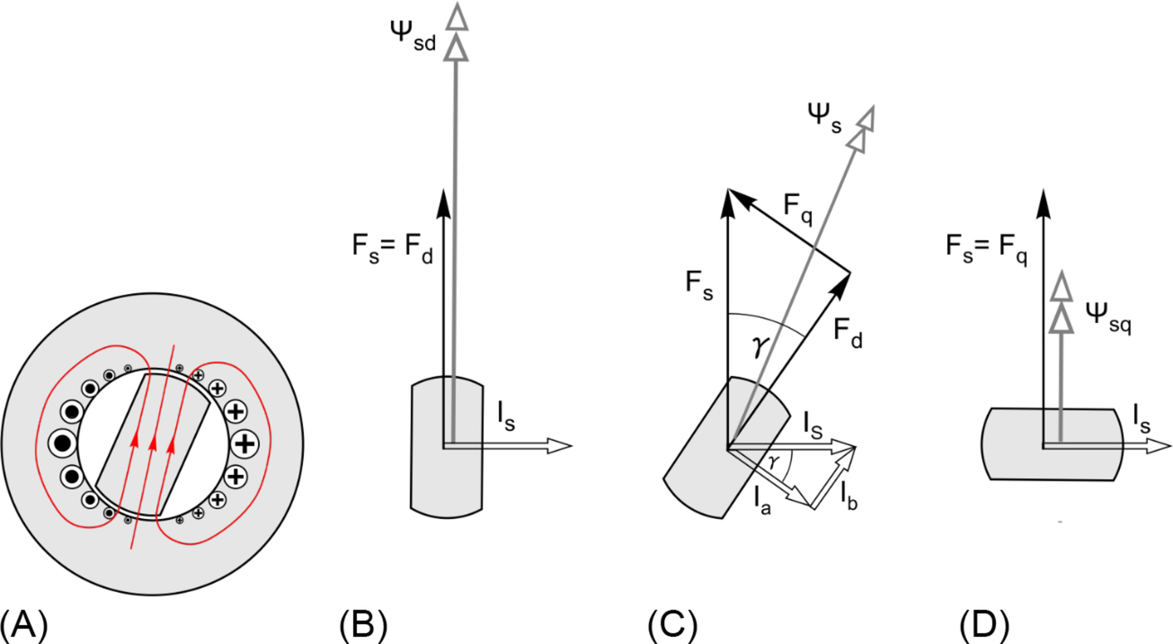
What we want to find is how the magnitude and phase of the stator flux linkage varies with the position of the rotor: if we know this, we can find the torque by applying the familiar ‘BIl’ approach used hitherto. The general position is shown in sketch (C), but it is best for us to establish some general ideas first by considering the limiting cases shown in sketches (B) and (D).
The peak of the stator current distribution (Is) lies on the horizontal axis, so the vector that represents the stator current distribution is horizontal and pointing to the right: this vector remains constant in all three sketches. The corresponding m.m.f. wave (Fs) is directed vertically upwards, and again it is constant in all three sketches.3 The suffices d and q refer to the direct and quadrature axes of the rotor, d being the low-reluctance axis, and q being the high reluctance path.
In sketch (B), for example, the stator m.m.f. Fs is directed along the rotor direct axis, and so it has been labelled Fd. The reluctance along the direct axis is low, so the stator flux linkage ψsd will be large. In contrast, in sketch (D) the same stator m.m.f. Fs is directed along the rotor's quadrature axis: it is therefore labelled Fq; and because the reluctance is relatively high, the corresponding stator flux linkage ψsq is relatively small.
In sketch (C), the stator m.m.f. vector has been resolved into direct and quadrature axis components. If each m.m.f. component acted on the same reluctance, the resultant flux linkage would be in phase with Fs. But the d-axis reluctance is much lower than the q-axis reluctance, so the resultant stator flux linkage (ψs) is shifted towards the direct axis. There are some similarities here with our previous discussions, where we saw that torque production required two fields to be displaced by an angle. This condition is met to a varying degree for all rotor positions between sketches (B) and (D), with m.m.f. and flux misaligned; but at the extremes both fields become co-phasal and the torque falls to zero.
In order to obtain the variation of torque with rotor angle and stator current, we need to form an expression equivalent to the ‘BIl’ product at the stator winding. Hitherto we have worked in terms of the flux density (B), but we can equally well use the flux linkage vector because we have specified that all quantities are sinusoidally distributed.
The sketch on the left in Fig. 9.10 is a repeat of the space vector diagram (C) in the previous sketch, and it shows the stator current distribution (Is) resolved into components Ia and Ib that are responsible for producing the m.m.f. components Fd and Fq, respectively. (It is important to point out that the resolved components of the current distribution vector in Fig. 9.10 should not be confused with the direct and quadrature axis currents that we will meet later in this chapter: the former are spatial quantities, represented here by outline arrows, while the latter are sinusoidal time-varying quantities, and are represented in time phasor diagrams by solid grey arrows.)
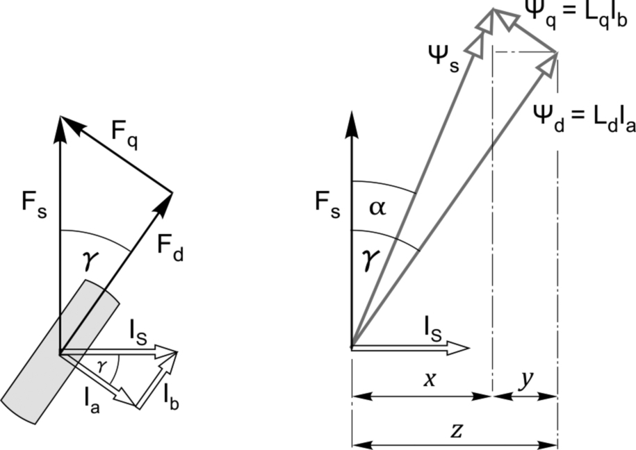
We need to find the component of the resultant flux linkage that is co-phasal with the current so that we can apply ‘BIl’. That component is represented by the distance x, but we do not know the angle α, so instead we find the difference between z and y, yielding the flux linkage component (equivalent to the ‘B' in BIl) as (LdIa sinγ − LqIb cos γ). The ‘I' part of BIl is of course Is. So we find that the torque (or strictly the force, but here we are seeking a general qualitative expression applicable to a generic motor, so dimensions are not considered) is given by
If we now express the current distributions Ia and Ib in terms of Is, i.e. Ia = Is cosγ and Ib = Is sin γ, the torque is given by
This simple expression shows that the torque depends on the square of the current, and is therefore the same for both positive and negative current: the torque is also a double-frequency function of the rotor angle, as we saw earlier. We already knew that in order to work at all, the rotor had to have saliency, but we now see that the torque is directly proportional to the difference between the direct and quadrature axis inductances, so that, broadly speaking, the greater the difference, the better. However, we will see later that this is not the only criteria, and that the ratio of the inductances also has important consequences for steady-state running.
In practical reluctance machines, as the current is increased, the iron begins to saturate and the torque assumes a more linear relationship with the current. In view of the importance of saturation, reluctance torque is predicted at the design stage using computer-based finite element analysis of the magnetic field distribution at each rotor position, and then using ‘BIl’ or the Maxwell stress method to find the torque. Finite element analysis also enables inductance variation to be obtained, so that the ‘coupled circuit’ approach (see Section 8.3) can then be used to predict all aspects of performance.
9.3.4 Salient pole synchronous motor
Looking back at Fig. 9.2, it is obvious that both rotors exhibit saliency, although it is much more pronounced in the one on the right. It is therefore to be expected that in addition to the excitation torque that depends on the rotor current (Section 9.3.1), there will also be reluctance torque (Section 9.3.3) which will be there even when there is no rotor current.
If we ignore saturation, the torque-angle relationship is obtained by superposing the excitation torque term and the reluctance torque term, giving the typical torque-angle curve shown in Fig. 9.11. The region to the right of peak torque in Fig. 9.11 is of no practical interest because it represents an unstable condition, but it is included to show one full cycle of the reluctance torque.

The most noticeable effect of the reluctance component is to increase the ‘stiffness’ (i.e. the gradient of the torque-angle curve) about the zero torque position, but it also reduces the stable operating region lying to the left of the (in this case, slightly increased) peak torque. The increased stiffness is generally beneficial, while the reduction in the stable region is unlikely to be significant because operation at such large load angles would not be possible without exceeding the rated current.
The relative magnitude of the excitation torque and the reluctance torque is a critical design consideration. Today substantial research is being undertaken to reduce the use of permanent magnets, resulting in motor designs with an increasing proportion of the total torque being reluctance torque: this is discussed further in Section 9.8.
9.3.5 Salient permanent magnet motor (‘PM/Rel’ motor)
In Section 9.3.4 we saw that for an excited rotor motor with rotor saliency, the reluctance torque acting alone caused the unloaded rotor to come to rest with the rotor direct axis aligned with stator m.m.f., i.e. at the same position as it would if the excitation torque acted alone. This is because the low-reluctance axis is the same as the excitation direct axis. The ‘stiffness’ of the torque-angle characteristic is increased by the presence of the reluctance torque, and depending on the relative magnitudes of the two components, the peak torque may also be increased, as shown in Fig. 9.11, so the combination is an attractive proposition.
The idea of replacing the rotor excitation circuit with simpler permanent magnets while continuing to exploit reluctance torque is clear in principle, but in practice is not as straightforward as might be expected. In order for the magnet flux to flow along the rotor direct axis (i.e. along a salient pole), a gap has to be inserted to accommodate the magnet, and the stronger the magnet, the longer the gap. This greatly increases the reluctance of the direct axis, which is the opposite of what we want in order to maximise the reluctance torque.
However, we have already talked about the move by many industries to reduce their dependency on rare earth magnets because of concerns over the global security of supply. This uncertainty, together with the incentive to provide low-cost motors for the burgeoning mass market (notably in hybrid electric vehicles), has led to renewed interest in motors that combine PM and reluctance torque. Compared with a purely PM motor, the aim is to achieve comparable performance with less magnet material: the ratio of PM torque to reluctance torque varies considerably (typically from 4:1 to as low as 1:1) depending on the detailed motor design and application, but in very simplistic terms, and stating the obvious, the less magnet material the higher the proportion of reluctance torque.
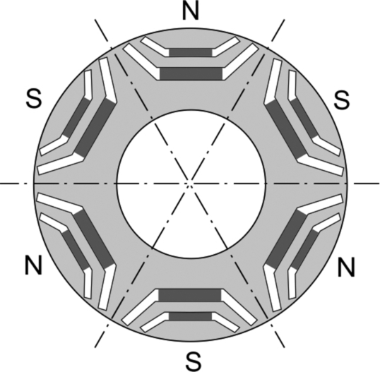
A typical six-pole rotor is shown in Fig. 9.12: it is basically a flux-guided reluctance motor rotor with buried permanent magnets sitting in the flux guides. Looking at the topmost N pole in Fig. 9.12 for example, its two magnets are effectively in series, and their direct (flux) axis is vertical. Apart from the air-gap, the main magnetic circuit external to each pair of magnets is of low reluctance through the core ‘iron’, so in this regard there is little compromise compared with PM-only design. However, for structural reasons there has to be a bridge of magnetic core material at the outer extremities of the flux guides, and this inevitably offers an attractive short-circuit for some of the magnet flux, which is thus diverted away from its useful path via the stator. This area remains saturated and unproductive in terms of torque.
As far as the reluctance aspect goes, the direct (low inductance) axis is shown by the chain-dotted lines, and the bridge referred to above again represents an unwanted short-circuit path for stator-produced flux, but in essence this is exactly as it would be in a flux-guided reluctance motor. If the reluctance torque acted alone, the unloaded rotor would come to rest with the stator m.m.f. aligned with the chain-dotted line, but if the PM acted alone, the unloaded rotor would come to rest with a N pole aligned with the stator m.m.f. So unlike the salient excited rotor motor, where the equilibrium positions coincided, we now have two distinct zero-torque positions, separated by 90° (elec.).
There is clearly potential confusion over which is the direct axis. On the face of it we have two rival contenders with conflicting claims: the reluctance camp would claim it was the chain-dotted line in Fig. 9.12, while the PM fans would argue it was an axis through the centre of the magnet poles. In practice the latter is usually preferred, i.e. the direct axis is defined in the same way as for a purely PM machine.
We can get a general idea of the shape of the overall torque-angle characteristic by superposing the separate reluctance and PM curves, as shown in Fig. 9.13, but we have to accept that this is only an approximation because it ignores the effects of saturation in the magnetic circuits.

The excited rotor case is included in Fig. 9.13 for comparison with the PM/Rel motor, and as we have already seen in Section 9.3.4, the resultant torque-angle curve for the excited rotor is stiffer about the stable zero-torque position, and the motoring and braking regions are symmetrically disposed, with equal maximum torque angles for motoring and braking of γm and γb, respectively.
Our aim is to highlight the fundamental differences between the torque-angle characteristics of the excited rotor motor and the PM/Rel motor, so we have arbitrarily chosen the reluctance and torque components to have the same amplitude. (In practice, an excited rotor motor would have much less reluctance torque, whereas the ratio of torque components for a PM/Rel motor could be higher or lower.)
The shift of 90° between the reluctance and PM curves results in different stable operating regions for the PM case, and also new zero-torque rest positions. The peak motoring and braking torques remain the same as for the excited rotor case, but they are no longer symmetrical about a single equilibrium rest position. The maximum motoring torque angle is indicated by γm, while the maximum braking torque is shown as γb. Hence when the drive requires the torque to change from maximum motoring torque to maximum braking torque, the control system (see Section 9.6) will reposition the stator current vector relative to the rotor by the angle κ shown in the lower diagram.
There is still a great deal of ongoing work and interest in this emerging technology, and it will be some time before optimised solutions for the various application areas finally emerge.
9.4 Utility-fed synchronous motors
Historically most synchronous machines were operated directly from the utility supply, so it is appropriate that we look first at the operation of synchronous machines assuming that the supply voltage and frequency are constant.
The physical picture involving spatially distributed m.m.f's, fluxes and current distributions in the previous section provided an explanation for the mechanism of torque production. We now shift attention into the time domain, and explore the steady-state behaviour when a synchronous motor is supplied from a balanced, constant voltage, sinusoidal supply. The stator current, which we held constant in the previous section, will now be one of the principal dependent variables, while the independent variables are the rotor excitation (if a wound rotor type) and the load on the shaft. The speed will be constant, so the power will be directly proportional to the torque.
Fortunately, predicting the current and power-factor drawn from the supply by a cylindrical-rotor or PM synchronous motor supplied from a balanced three-phase supply is possible by means of the per-phase a.c. equivalent circuit shown in Fig. 9.14. To arrive at such a simple circuit inevitably means that approximations have to be made (notably in relation to saturation in the magnetic circuit), but we are seeking only a broad-brush picture, so the circuit is perfectly adequate.

In this circuit Xs (known as the synchronous reactance, or simply the reactance) represents the effective inductive reactance of the stator phase winding; R is the stator winding resistance; V is the applied voltage; and E is the e.m.f. induced in the stator winding by the rotating flux produced either by the d.c. current on the rotor or the permanent magnet.
The term ‘effective’ reactance applied to Xs reflects the fact that the magnitude of the flux wave produced by balanced currents in each of the three phase windings is 1.5 times larger than the flux that would be produced by the same current in only the one winding. The effective inductance of each phase (i.e. the ratio of flux linkage to current) is thus 1.5 times the self inductance of each phase winding, and consequently the synchronous reactance Xs = 1.5 X, where X is the reactance of one phase. For the benefit of readers who are familiar with the parameters of the induction motor, it should be pointed out that Xs is equal to the sum of the magnetising and leakage reactances, but because the effective air-gap in synchronous machines is usually larger than in induction motors, their per-unit synchronous reactance is usually lower than that of an induction machine with the same stator winding.
It may seem strange that in the previous section we were talking about both the rotor flux and the stator flux, but now, we refer to the e.m.f. induced by the rotor flux, and seem to have ignored the e.m.f. due to the rotating stator (armature) flux. Needless to say, we have not forgotten the stator flux, because we are following the conventional approach in which the self-induced e.m.f. due to the resultant stator flux (which is proportional to the stator current) is represented by the voltage (IXs) across the inductive reactance, Xs.
At this point, readers who are not familiar with a.c. circuits and phasor diagrams will inevitably be disadvantaged, because discussion of the equivalent circuit and the associated phasor diagram greatly assists the understanding of motor behaviour. We have included a brief resume of phasors in Section 9.4.3, but we have also summed up the lessons learned in each case, so that readers who have been unable to absorb the theoretical underpinning will not be seriously handicapped.
9.4.1 Excited rotor motor
Our aim is to find what determines the current drawn from the supply, which from Fig. 9.14 clearly depends on all the parameters therein. But for a given machine operating from a constant-voltage, constant-frequency supply, the only independent variables are the load on the shaft and the d.c. current (the excitation) fed into the rotor, so we will look at the influence of both, beginning with the effect of the load on the shaft.
The speed is constant and therefore the mechanical output power (torque times speed) is directly proportional to the torque being produced, which in the steady-state is equal and opposite to the load torque. Hence if we neglect all the losses in the motor (and in particular we assume that the resistance R is negligible), the electrical input power is also determined by the load on the shaft. The input power per phase is given by VI cos ϕ where I is the current and the power-factor angle is ϕ. But V is fixed, so the in-phase (or real) component of input current (I cos ϕ) is determined by the mechanical load on the shaft. We recall that, in the same way, the current in the d.c. motor (Fig. 3.6) was determined by the load. This discussion reminds us that although the equivalent circuits in Figs. 9.14 and 3.6 are very informative, they should perhaps carry a ‘health warning’ to the effect that one of the two independent variables (the load torque) does not actually appear explicitly on the diagrams.
Turning now to the influence of the d.c. excitation current, at a given supply frequency (i.e. speed) the utility-frequency e.m.f. (E) induced in the stator is proportional to the d.c. field current fed into the rotor. If we wanted to measure this e.m.f. we could disconnect the stator windings from the supply, drive the rotor at synchronous speed by an external means, and measure the voltage at the stator terminals, performing the so-called ‘open-circuit’ test. If we were to vary the speed at which we drove the rotor, keeping the field current constant, we would of course find that E was proportional to the speed. We discovered a very similar state of affairs when we studied the d.c. machine (Chapter 3): its induced motional or ‘back’ e.m.f. (E) turned out to be proportional to the field current, and to the speed of rotation of the armature. The main difference between the d.c. machine and the synchronous machine is that in the d.c. machine the field is stationary and the armature rotates, whereas in the synchronous machine the field system rotates while the stator windings are at rest: in other words, one could describe the synchronous machine, loosely, as an ‘inside-out’ d.c. machine.
We also saw in Chapter 3 that when the unloaded d.c. machine was connected to a constant voltage d.c. supply, it ran at a speed such that the induced e.m.f. was (almost) equal to the supply voltage, so that the no-load current was almost zero. When a load was applied to the shaft, the speed fell, thereby reducing E and increasing the current drawn from the supply until the motoring torque produced was equal to the load torque. Our overall conclusion was the simple statement that if E is less than V, the d.c. machine acts as a motor, while if E is greater than V, it acts as a generator.
The situation with the synchronous motor is similar, but now the speed is constant and we can control E independently via control of the d.c. excitation current fed to the rotor. We might again expect that if E was less than V the machine would draw-in current and act as a motor, and vice-versa if E was greater than V. But we are no longer dealing with simple d.c. circuits in which phrases such as ‘draw in current’ have a clear meaning in terms of what it tells us about power flow. In the synchronous machine equivalent circuit the voltages and currents are a.c., so we have to be more careful with our language and pay due regard to the phase of the current, as well as its magnitude. Things turn out to be rather different from what we found in the d.c. motor, but there are also similarities.
Phasor diagram and power-factor control
We will begin by looking at how the e.m.f. (E) influences the behaviour of the motor when it is running without any shaft load. By excluding one of the two independent variables (i.e. the load torque), we can highlight the role of the other independent variable (the rotor current) in relation to the excitation or flux producing requirement.
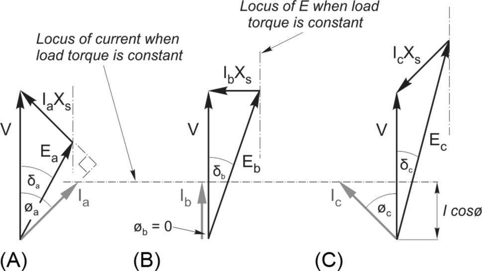
If we neglect winding resistance, iron loss and frictional losses, the input electrical power is equal to the mechanical output power, so in this case the input power will be zero, which means that the ‘real’ component of the phase current (i.e. the component in phase with V) will be zero, and the machine will therefore always be ‘reactive’ as viewed from the utility supply. The four sketches in Fig. 9.15 show how the input current (and thus the effective reactance) varies with the induced e.m.f. (E): they embody the result of applying Kirchoff's voltage law to the equivalent circuit in Fig. 9.14, i.e. V = E + IR + jIXs, but with R neglected, so the phasor diagram simply consists of the volt-drop IXs (which leads the current (I) by 90°) added to E to yield V.

In sketch (A), the rotor current (and hence E) is zero, so according to Fig. 9.14 the motor will look like a pure inductance when viewed from the supply, and the current (Io, the ‘o’ denoting no-load) will be given by V/Xs, where Xs is the synchronous reactance at the frequency of the supply. The large current (perhaps of the order of 60% of the full-load current in a large motor) is lagging by 90°, so the motor is therefore consuming reactive power only. In this extreme case the motor might be described as un-excited because there is no rotor current, but in fact a rotating field must be set up to induce an internal e.m.f. equal to the terminal voltage, and in this case all of the necessary m.m.f. is provided by the stator current in each phase. We discussed a similar state of affairs when we looked at the unloaded induction motor, where it emerged that the no load current lagged the voltage by almost 90°, and was called the ‘magnetising’ current, because it was responsible for setting up the rotating flux wave. Here the use of the term ‘excitation’ harks back to the d.c. machine, but the word ‘magnetising’ would be equally suitable.
In case (B), the rotor current is sufficient to produce a flux wave that in turn induces an e.m.f. of half the terminal voltage, so now the stator current is only half of that in (A) because it only has to make up the shortfall of excitation. The reactive power is now reduced, but it is still lagging. This condition, where the induced e.m.f. E is less that V, is usually referred to as ‘under-excited’.
In the special case shown in Fig. 9.15C, the induced e.m.f. is equal to the applied voltage, the current is zero, and the motor appears as an open circuit to the supply.
Finally, the ‘over-excited’ case is shown in sketch (D). The rotor excitation is now 50% larger than required to balance the voltage V, so the stator current reverses in phase and now opposes the rotor excitation. The current now leads by 90°, and the motor can equally well be viewed as exporting lagging VArs or consuming leading VArs, i.e. it looks capacitive. (When synchronous machines were operated with both ends of the rotor shaft sealed off, so that no mechanical power was involved, they were known as ‘compensators’, with the ability to ‘look like’ either an inductor or a capacitor, and until the advent of power electronics they were used for regulating purposes in power systems.)
We now turn to the more important practical case where the motor is supplying mechanical output power, and again we will investigate how the magnitude of the e.m.f. influences behaviour, with the aid of the phasor diagrams in Fig. 9.16.
The first point to clarify is that our sign convention is that motoring corresponds to positive electrical input power to the machine. The power is given by VI cos ϕ, so when the machine is motoring (positive power) the angle ϕ lies in the range ± 90°. If the current lags or leads the voltage by more than 90° the machine will be generating.
The sketches in Fig. 9.16 correspond to low, medium and high values of the induced e.m.f. (E), the shaft load (i.e. mechanical power) being constant. As discussed above, if the mechanical power is constant, so is I cos ϕ, and the locus of the current is therefore shown by the horizontal dashed line. The load angle (δ), discussed earlier, is the angle between V and E in the phasor diagram.
Fig. 9.16A represents an under-excited condition where the field current has been set so that the magnitude of (E) is less than V, which leads to a relatively large lagging reactive current component. When the field current is increased (increasing the magnitude of E) the magnitude of the input current reduces and it moves more into phase with V: the special case shown in Fig. 9.16B shows that the motor can be operated at unity power-factor if the field current is suitably chosen.
A brief digression is appropriate at this point to relate the time phasor diagram to the space phasors in Fig. 9.6. We imagine the space phasors to be rotating at the synchronous speed, in which case each of them gives rise to an induced motional e.m.f. in the stator. The rotor space phasor (FR) produces E (proportional to the d.c. current in the rotor), and the stator space phasor (FS) produces an e.m.f. (which is proportional to the armature current) that we represent by the voltage IXs. The resultant of these two space phasors (F) produces the resultant flux linkage at the stator winding (ψs), which must induce the terminal voltage, V, so, depending on the magnitude of E, the armature current adjusts accordingly.
The unity power factor case shown in (B) represents the minimum current for the given power (or torque), when the terminal voltage V and frequency are fixed. The corresponding space phasor triangle will have an area determined by the torque, a resultant (F) that is fixed, and FR adjusted so as to minimise FS, which will be achieved when the angle α in Fig. 9.6 is 90° and FS is perpendicular to F. This represents the optimum condition for maximising torque when the resultant and rotor fluxes are specified, and the space phasor diagram will then be a scaled version of Fig. 9.16B.
Returning to Fig. 9.16C, the field current is considerably higher (the ‘over-excited’ case) which causes the current to increase again but this time the current leads the voltage and the power-factor is cosϕc, leading. We see that we can obtain any desired power-factor by appropriate choice of rotor excitation, and in particular we can operate with a leading power-factor, a freedom not afforded to users of induction motors.
When we studied the induction motor we discovered that the magnitude and frequency of the supply voltage V governed the magnitude of the resultant flux density wave in the machine, and that the current drawn by the motor could be considered to consist of two components. The real (in-phase) component represented the real power being converted from electrical to mechanical form, so this component varied with the load. On the other hand the lagging reactive (quadrature) component represented the ‘magnetising’ current that was responsible for producing the flux, and it remained constant regardless of load.
The stator winding of the synchronous motor is essentially the same as the induction motor, so, as discussed above, it is to be expected that the resultant flux will be determined by the magnitude and frequency of the applied voltage. This flux will therefore remain constant regardless of the load, and there will be an associated requirement for magnetising m.m.f. But as we have already seen, we have two possible means of providing the excitation m.m.f., namely the d.c. current fed into the rotor and the lagging component of current in the stator.
When the rotor is under-excited, i.e. the induced e.m.f. E is less than V (Fig. 9.16A), the stator current has a lagging component to make up for the shortfall in excitation needed to yield the resultant field that must be present as determined by the terminal voltage, V. With more field current (Fig. 9.16B), however, the rotor excitation alone is sufficient and no lagging current is drawn by the stator. And in the over-excited case (Fig. 9.16C), there is so much rotor excitation that there is effectively some reactive power to spare and the leading power-factor represents the export of lagging reactive power that could be used to provide excitation for induction motors elsewhere on the same system, thereby raising the overall system power factor. As might have been expected, these observations about the role of the excitation line up nicely with what we saw when we looked at the no-load behaviour.
To conclude our look at the excited rotor motor we can now quantify the torque. From Fig. 9.16, the real power is given by

The speed is constant, so the torque is also given by an expression of the form

This agrees with the conclusion we reached in Section 9.3.1, where we saw that the torque depended on the product of the resultant field (here represented by V), the rotor field (here represented by E) and the sine of the load angle between them (δ). We note that if the load torque is constant, the variation of the load-angle (δ) with E is such that E sin δ remains constant. As the rotor excitation is reduced, and E becomes smaller, the load angle increases until it eventually reaches 90o, at which point the rotor will lose synchronism and stall. This means that there will always be a lower limit to the excitation required for the machine to be able to transmit the specified torque. This is just what our simple mental picture of torque being developed between two magnetic fields, one of which becomes very weak, would lead us to expect.
9.4.2 Permanent magnet motor
Although the majority of permanent magnet motors are supplied from variable-frequency inverters, some are directly connected to the utility supply, and we can again explore their behaviour using the equivalent circuit shown in Fig. 9.14. Because the permanent magnet acts as source of constant excitation, we no longer have control over the magnitude of the induced e.m.f. (E), which now depends on the magnet strength and the speed, the latter being fixed by the utility frequency. So now we only have the load torque as an independent variable, and, as we saw earlier, because the supply voltage is constant, the load torque determines the in-phase or work component of the stator current (Icos ϕ) as indicated in the phasor diagrams in Fig. 9.16.
In order to identify which of the three diagrams in Fig. 9.16 applies to a particular motor we need to know the motional e.m.f. (E) with the rotor spinning at synchronous speed and the stator open-circuited. If E is less than the utility voltage, diagram (A) applies; the motor is said to be under-excited; and it will have a lagging power-factor that worsens with load. Conversely, if E is greater than V, (the over-excited case) diagrams (B) or (C) are typical, and the power factor will be leading.
9.4.3 Reluctance motor
Time phasor diagrams for one phase winding under no-load and loaded conditions are shown in Fig. 9.17A and B, respectively, and in each case the time phasors of the flux linkage have been shifted to the right to avoid congestion with the voltages and current. These flux phasors can be compared with the space vectors shown in Fig. 9.10. Once again, resistance has been neglected in the interests of simplicity.
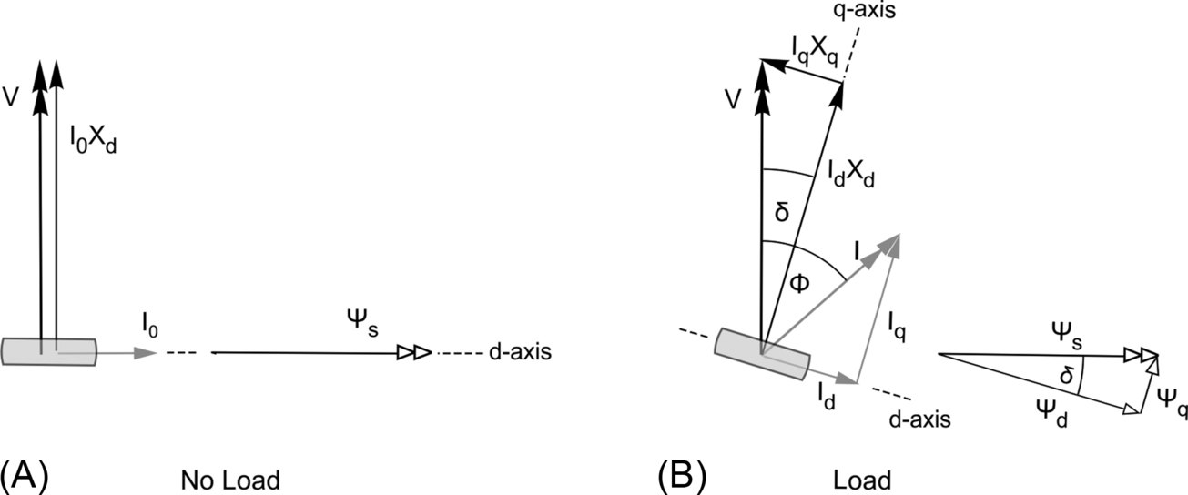
Two novel features of Fig. 9.17 are firstly the resolved current components Id and Iq, and secondly the incongruity of finding a sketch of a salient rotor in a diagram that supposedly represents time-varying electric circuit quantities. We will therefore break off from the specifics of the reluctance motor, firstly to refresh our understanding of the properties of time phasors, and secondly to justify the presence of the rotor in Fig. 9.17.
The purpose of a phasor diagram is to provide an efficient graphical way of representing the steady-state inter-relationship between quantities that vary sinusoidally in time. We picture all phasors to be rotating anticlockwise at a constant speed and completing one revolution per cycle of the supply. The length of each phasor is proportional to the amplitude (or more usually r.m.s. value) of the quantity represented, and its angular position represents its phase with respect to the other quantities. The projection of the tip of each phasor onto the vertical axis of the diagram then indicates its instantaneous value, which will, of course, vary sinusoidally in time: and if we were to arrange for a pen to be fixed to the tip of each phasor, and for the pen to bear on an endless strip of paper moving at a steady speed from left to right behind the rotating phasor, the trace on the paper would be a sinewave.
In this book, time phasor diagrams represent what is happening inside one of the stator windings, which by definition means that we are in a stationary reference frame, in which two distinct types of quantity may be represented. Firstly, there are the terminal voltages and currents (that we could measure with a voltmeter and ammeter), and the various ‘internal to the equivalent circuit’ voltages and currents that together make up the terminal quantities. These are single valued time functions which have no spatial meaning associated with them. But we also display quantities such as flux linkages that are sinusoidally distributed in space: this is justified because the rotating flux linkage space phasor manifests itself in the winding as a sinusoidally time-varying effect, the rate of change of which results in an induced voltage.
For the diagrams to be meaningful, it hardly needs saying that all quantities of the same kind (e.g. voltages) must be drawn to the same scale, while physically different quantities (e.g. currents) can be drawn to a different but consistent scale.
In the light of the above discussion, we would not expect to see the ghostly outline of a salient pole rotor superimposed on a diagram such as that in Fig. 9.17, and we are not about to argue that a rotor is a time-varying quantity. But the rotor does rotate by one pole-pair for each electrical cycle, and we have seen in the discussion of torque production (in Section 9.3.3) that in the steady state the rotor has a fixed angular relationship with the resultant flux phasor, so including it is not so fanciful after all, and as we will now see, it helps us to understand the phasor diagram by locating the direct and quadrature axes, and hence throwing light on the currents Id and Iq.
In Section 9.3.3 we defined the low reluctance path through the rotor as the direct axis, and the higher reluctance path as the quadrature axis. Hence when we include the rotor outline in a phasor diagram we implicitly define the direct axis (for example it is horizontal in Fig. 9.17A) and the quadrature axis (vertical). (We adopt the most widely-used convention, with the quadrature axis leading the direct axis by 90°, but readers should not be surprised to find textbooks that use alternatives.)
Returning now to the discussion of the reluctance motor phasor diagram in Fig. 9.17A that represents the unloaded motor, we choose the constant supply voltage V as reference, and follow the usual practice by drawing it vertical.
As we have seen for the induction and synchronous machines, the resultant flux linkage ψs is determined by the supply voltage and frequency, and the in-phase component of current (I cos ϕ), is solely determined by the load torque. The reluctance motor has no rotor excitation, so the stator current always has to draw an excitation or magnetising component.
At no load, (Fig. 9.17A, there is no in-phase component of current, and so the no-load current Io is all excitation or magnetising current, and it produces the flux linkage ψs which is in time phase with the current, and in turn induces the e.m.f. which must equal V. We have encountered these flux-e.m.f. relations several times already.
Where there is no saliency, we chose to represent the self-induced e.m.f. by means of the synchronous reactance voltage drop IXs. But with saliency, we have seen that for a given stator current, the self flux linkage (and hence the inductance) depends on the angular position of the rotor. We therefore introduced two new inductances Ld and Lq to assist analysis. Ld represents the inductance when the direct axis of the rotor is aligned with the m.m.f. axis of the stator phase, and Lq is the inductance when the rotor direct axis is perpendicular to the phase axis. The corresponding steady-state reactances are Xd and Xq, but it is not immediately obvious how these are to be reflected in the phasor diagram. This is where the rotor outline becomes invaluable.
Referring back to Fig. 9.10, we learned that torque is proportional to the sine of (twice) the space angle (δ) between the direct axis and the resultant flux, so we know that at no-load, the flux is along the direct axis. As the flux wave rotates, the rotor remains in synchronism with the flux, so we could legitimately add another ‘phasor arrow’ to the time diagram labelled ‘rotor direct axis’: in practice, it is more graphic to put a rotor outline, as shown in Fig. 9.17.
We now know that at no-load, the direct axis of the rotor is aligned with the flux wave, so this determines the rotor outline under no-load conditions as being in time phase with the flux, i.e. horizontal in Fig. 9.17A. The stator m.m.f. is thus entirely directed along the direct axis, and we therefore refer to the corresponding current as the ‘direct axis’ current. In this special (no-load) case all of the current is d-axis current (I0 = Id).
The flux produced by the d-axis current is determined by the d-axis inductance, and the e.m.f. induced by the flux is therefore related to the current by the d-axis reactance. The volt-drop that we choose to represent this e.m.f. is the phasor IdXd in Fig. 9.17A.
The phasor diagram when the motor is on load is shown in Fig. 9.17B, again with the voltage V as reference, and as at no load, the resultant flux remains the same because it has to induce an e.m.f. equal to V. The resultant flux is no longer on the direct axis, and the rotor is lagging the flux by the load angle (δ). The load torque determines the component of current that is in phase with V (i.e. IcosΦ—not shown), but the reactive component that finally determines the phase of the current depends on the two reactances, as explained below.
The significance of the current components Id and Iq should now be clear. The m.m.f. associated with Id acts along the direct axis of the rotor, and produces a flux linkage ψd that is given by LdId, and a corresponding self-induced e.m.f. given by Id Xd. We refer to Id as the flux producing, magnetising or excitation component of the current, and as we have seen, at no load, all of the input current is direct axis current.
Conversely, Iq is the torque-producing component of current: its associated m.m.f acts along the quadrature axis, producing a flux linkage component ψq given by LqIq and a corresponding component of self-induced e.m.f. given by IqXq.
It is important to reiterate that the time phasor diagram represents voltages and currents that are varying sinusoidally in time, in a stationary reference frame. In particular, the direct and quadrature components Id and Iq of the phase current that we have just discussed are not to be confused with the transformed variables id and iq in the rotating reference frame that we discussed in Chapter 8. The latter are, under steady-state conditions, constant (‘d.c.’) currents that produce at the rotor the same m.m.f. that is produced by the a.c. currents in the stator windings. We will return to the transformed currents later when we deal with field-oriented control.
To obtain the output power per phase from the phasor diagram is a straightforward but tedious process, the result of which is that the power is given by

The speed is constant, so this expression also represents the relationship between the torque and the load angle, δ. Physically, as we have seen, δ is the angle between the resultant rotating field and the direct axis of the rotor, i.e. the ‘lag’ of the rotor with respect to the resultant field, and it therefore bears some similarity with the load angle of motors that have rotor excitation.
The static analysis in Section 9.3.3 showed that the torque was proportional to (Ld − Lq) and sin 2γ, where γ is the torque angle, whereas here we find that the torque is proportional to ![]() where δ is the load angle. The differences stem from our choices of the contrasting constraints between the static and steady running cases: in the former, the current was kept constant, and the resultant flux varied according to the rotor angle, while in the latter, the voltage and frequency force the resultant flux to be constant, and the current has to adjust accordingly.
where δ is the load angle. The differences stem from our choices of the contrasting constraints between the static and steady running cases: in the former, the current was kept constant, and the resultant flux varied according to the rotor angle, while in the latter, the voltage and frequency force the resultant flux to be constant, and the current has to adjust accordingly.
9.4.4 Salient pole motor
Modelling the salient pole motor is based on an equivalent circuit similar to that for the smooth rotor motor in Fig. 9.14, with an induced e.m.f. E due to the rotor excitation. But because of the saliency and the consequent reluctance component of torque, the single synchronous reactance (Xs) has to sub-divided into a direct-axis reactance (Xd) and a quadrature axis reactance (Xq). These reactances are the same as we discussed in the previous section.
The time phasor diagram is essentially a combination of those shown in Figs. 9.16 and 9.17, and again resistance has been neglected. Constructing the diagram involves resolving the current into direct and quadrature axis components, before the reactive volt drops IdXd and IqXq can be identified. We will not go into detail, but typical phasor diagrams for over-excited and under-excited conditions are shown in Fig. 9.18A and B, respectively, both sketches being for the same output power or torque.

In the over-excited case, the current is leading, i.e. lagging Vars are being exported, whereas in the under-excited case additional lagging Vars are needed to supplement the excitation provided by the rotor current.
The power and torque can be derived from Fig 9.18 in terms of the controllable variables (V, E, and the load torque), but the lengthy manipulations are not necessary and we will simply quote the well-known result that the torque is given by the expression

The first term is the same as that for the round-rotor excited machine that we saw earlier, but with Xd replacing X, and the second term is the same as we found for the reluctance motor. We note that, even when the rotor excitation is zero (i.e. E = 0), the salient pole motor can produce torque by reluctance action alone, but needless to say, the reluctance torque depends on the degree of saliency: a motor with a rotor such as that in Fig. 9.2A might produce 5% of its torque via reluctance action, whereas the reluctance term for the type of rotor in Fig. 9.3B could easily contribute 30% or more.
9.4.5 Starting on utility supply
It should be clear from the discussion of how torque is produced, that unless the rotor is running at the same speed as the rotating field, no steady torque can be produced. If the rotor is running at a different speed, the two fields will be sliding past each other, giving rise to a pulsating torque with an average value of zero. Hence a basic synchronous machine is not self-starting, and some alternative method of producing a run-up torque is required.
Most line start synchronous motors, designed for direct connection to the utility supply, are therefore equipped with some form of rotor cage, similar to that of an induction motor, in addition to the main field winding. When the motor is switched onto the supply, it operates as an induction motor during the run-up phase, until the speed is just below synchronous. The excitation is then switched on, and as long as the load is not too high, the rotor is able to make the final acceleration and ‘pull-in’ to synchronism with the rotating field. Because the cage is only required during starting, it can be short-time rated, and therefore comparatively small. Once the rotor is synchronised, and the load is steady, no currents are induced in the cage, because the slip is zero. The cage does however come into play when the load changes, when it provides an effective method for damping out the oscillations of the rotor as it settles at its new steady-state load angle.
Large motors will tend to draw a very heavy current during run-up, perhaps 6 or more times the rated current, for many tens of seconds, or longer, so some form of reduced voltage starter is often required (see Chapter 6). Sometimes, a separate small or ‘pony’ motor, is used simply to run-up the main motor prior to synchronisation, but this is only feasible where the load is not applied until after the main motor has been synchronised.
9.5 Variable frequency operation of synchronous motors
Just as we have seen in Chapters 7 and 8 for the induction motor, once we interpose a power electronic converter between the utility supply and the machine we introduce new levels of performance and lose most of the inherent drawbacks which we find when the motor is directly connected to the utility supply.
Most obviously, a variable frequency converter frees the synchronous machine from the fixed-speed constraint imposed by utility-frequency operation. The obvious advantage over the inverter-fed induction motor is that the speed of the synchronous motor is exactly determined by the supply frequency whereas the induction motor always has to run with a finite slip. On the down side, we lose the ability of the excited rotor motor to vary the power factor as seen by the utility supply.
In principle, a precision frequency source (oscillator) controlling the inverter switching is all that is necessary to give precise speed control with a synchronous motor, while speed feedback is essential to achieve such accuracy with an induction motor. In practice however, we seldom use open-loop control, where the voltage and frequency are generated within the inverter, and are independent of what the motor does. Instead, field-oriented control, almost identical to that described for the inverter-fed induction motor, predominates (see Section 9.6). The principal advantage of FOC is that it allows us to control the torque and flux components of the stator current independently, and in the case of the PM motor it prevents the motor from losing synchronism with the travelling field by locking the supply frequency to the speed of the rotor.
However, in the steady state, an observer looking at the stator voltage and current would see steady state sinusoidal waveforms, and would be unaware of the underlying control mechanism. We can therefore study the steady-state behaviour using the equivalent circuit in much the same way as we did with the utility-fed PM motor. We will continue to ignore resistance because this makes the phasor diagrams much simpler to understand without seriously compromising our conclusions.
In this section we again use the phasor diagram showing voltages and current, but we also include the time varying fluxes in order to emphasise the link between the two sets of variables.
As before, we imagine the flux produced by the magnet and the flux produced by the stator as if they existed independently, although in reality there is only one resultant flux. We have seen previously that because the fluxes rotate in synchronism, the magnitude of the torque depends on the product of the two field strengths and the angle between them: when aligned, the torque is zero, and when perpendicular, it is maximum. This is equivalent to saying that the torque is maximum when the stator current wave is aligned with the magnet flux wave, which is the traditional ‘BIl’ picture.
When we discussed the various utility-connected motors in Section 9.4, we saw that because the voltage and frequency were fixed, the resultant (stator) flux was constant. For the excited-rotor motor, the rotor current could be adjusted to achieve a power factor of unity, but for the PM motor, in which the rotor excitation is constant, the stator current adjusted itself to satisfy the requirement for the resultant flux to be constant, and as a result we had no control over the power factor.
With an inverter-fed motor we gain control of both the stator voltage and frequency, so that together with the load torque we now have three independent variables in the case of the PM motor, or four for the excited rotor machine. Despite the recent re-emergence of the inverter fed reluctance motor, the majority of inverter-fed synchronous motor drives, employ PM motors, so we will concentrate on their behaviour for the remainder of this section.4
9.5.1 Phasor diagram of PM motor
The general diagram (Fig. 9.19) is for an under-excited case, i.e. at the speed in question, the open circuit e.m.f. (E) is less than the terminal voltage. The red and green regions within the stylised rotor outline indicate the poles of the magnet, and thus define the direct axis (horizontal) in the diagram. The magnet flux (Φmag) remains constant, so we choose it as our horizontal reference throughout this and the following sections.
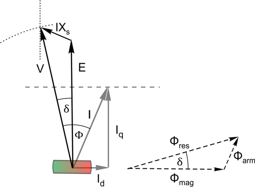
Fig. 9.19 is similar to Fig. 9.16, but we have chosen to add the flux phasors in order to lay the groundwork for the later discussion of field-oriented control. As explained below, the flux and voltage triangles are similar, and each flux is proportional to the corresponding m.m.f. (see Fig. 9.6): for example, the rotor flux (φmag) corresponds with the rotor m.m.f. (FR in Fig. 9.6).
E is the open circuit e.m.f. produced by the magnet flux (φmag): it is proportional to the magnet flux and the speed, which is proportional to the stator frequency, ω. Once we specify the frequency the magnitude of E is known, so we can start the left hand side of the diagram with E drawn vertically because, as previously discussed, the induced e.m.f. leads the magnet flux by 90°.
φarm is the flux that would be set up if the armature (stator) current existed alone. We are assuming no saliency, so the magnitude and direction of this flux depend only on the magnitude and phase of the stator current (I).
φres is the resultant (‘the’) flux. With resistance ignored, this flux is effectively determined by the applied voltage and frequency, as we have seen several times earlier in this book, so in the phasor diagram, the magnitude of this flux is proportional to, and in quadrature with, V.
As usual, the self-induced e.m.f. from the stator flux is modelled by means of the voltage across the effective stator inductive reactance, Xs, so in the phasor diagram the voltage IXs leads the current by 90°.
V is the applied stator voltage, here regarded as an independent variable, and I is the resulting stator current. The stator phasor equation is V = E + IXs (the terms being vectors, of course), or V = E + jIXs for those who prefer the complex notation.
The other independent variable is the load torque, which is our next consideration in developing the diagram. We dealt with the same matter in relation to Fig. 9.16, where the utility supply voltage was constant. But now the voltage is not fixed, so we will take a different approach that focuses instead on how we need to control the current in order to achieve the required torque in the most efficient way. This will assist us in understanding the strategy employed in the torque control loop of a PM motor drive, which we look at later in this chapter.
In the steady state, the motor torque must equal the load torque. The motor torque is proportional to the product of the current (I), the magnet flux (φmag), and the sine of the angle between them (δ), or in other words to the product of the magnet strength and the component of current at right angles to the magnet flux. Hence the load torque determines the torque component of the stator current (Iq), as shown in Fig. 9.19. The locus of the current I is then the horizontal dashed line, and the locus of V is the vertical dotted line as shown in Fig. 9.19. So when we finally specify the magnitude of V (shown by the dotted arc), the intersection of the arc and vertical line fixes the phase of the stator current, thereby specifying the direct axis component Id and finalising the diagram.
The current component in phase with E is the useful or torque component Iq, while the component in phase with the magnet flux is the flux component Id. The area of the flux triangle is proportional to the product of Iq and φmag, and thus the area provides an immediate visual indication of the torque.
If we adjust V so that the stator current is in phase with E, (i.e. the flux component Id is zero), we get the maximum torque per ampere of stator current, and thus the minimum stator copper loss for that particular torque: if iron loss is ignored, this would be the most efficient condition.
It is important to stress that the conclusion that we have reached—that the torque is proportional to the quadrature component of current - is not restricted to the steady-state condition that we have assumed so far, and is in fact the basis of the field-oriented control system that we will discuss in Section 9.6.
Alternative expressions for the power per phase can be derived from the geometry of the phasor diagram with the aid of a few construction lines. The first is identical to that obtained for the excited rotor motor, i.e. P = ![]() , while the second, which is more appropriate when the current is being controlled directly, is P = EIq. The second equation is of exactly the same form as we found for the d.c. machine in Chapter 3.
, while the second, which is more appropriate when the current is being controlled directly, is P = EIq. The second equation is of exactly the same form as we found for the d.c. machine in Chapter 3.
Before we move on, we should note that because we looked at an example where the applied voltage is just a bit larger than E, the current turned out to be of modest amplitude and at a reasonable power-factor angle. However, if we had specified a much higher V, we would find that the current would have had a much larger lagging flux component (with the same torque component, determined by the load), and a much worse power factor. And conversely, a much smaller applied voltage would result in a large leading power-factor current. This behaviour is in line with what we have already seen, and neither condition is desirable because of the increased copper loss.
9.5.2 Variable speed and load conditions
In Section 9.7 we will look at the torque-speed and performance capabilities of the inverter-fed PM synchronous motor, and we will find that, as with the d.c. drive and the induction motor drive there is a so-called constant torque region that extends up to base speed, within which full rated torque is available on a continuous basis. And in common with the other drives, at higher speeds there is a field weakening region where the maximum available torque is reduced. However, the usual constraints imposed by the maximum supply voltage and allowable continuous stator current may result in more serious restrictions on operation in this region than we have seen with other drives, including the likelihood that only intermittent operation may be possible.
Given the number of parameters involved and their variation between motor designs, it is only possible for us paint a broad picture, so we will look at one hypothetical machine and use it to provide an insight into some of the issues involved. We will focus on what can be learned from the phasor diagrams for three steady-state conditions, two in the constant-torque region and one in field weakening. The lessons learned will prove invaluable when we move on to study field-oriented controlled drives.
For convenience in calculations in relation to the steady-state phasor diagrams we will take the open-circuit e.m.f. E at the base speed (ωB) to be 1 p.u. (In practice, the rated applied voltage is usually taken as 1 p.u., but there is no reason why any other value should not be chosen.) We will assume that the reactance of the winding (X) at the base speed is 0.3 p.u. (which means that at rated current (and rated frequency) the voltage across the reactance is 0.3 times the rated voltage).
Full load (full torque at base speed)
By full load we mean that the machine is running at base speed and delivering its full rated torque. We saw above that the current depended on the applied voltage, and that in particular if we apply the right voltage we can minimise the current. This is what we do in field oriented control, so the diagram (Fig. 9.20) represents this condition.

We should note that the stator current has zero flux component, and so the armature flux is perpendicular to the magnet flux, i.e. in the optimum torque-producing position. We will define the current in this situation as 1 p.u., so the volt-drop across the reactance is ![]() From the property of the right-angled triangle, V turns out to be 1.04 p.u., and because we have defined this as the rated power condition, we will regard 1.04 V as the maximum voltage that the inverter can produce. If iron loss is neglected, this condition is the most efficient state for the given current and torque, because the stator copper loss is minimised.
From the property of the right-angled triangle, V turns out to be 1.04 p.u., and because we have defined this as the rated power condition, we will regard 1.04 V as the maximum voltage that the inverter can produce. If iron loss is neglected, this condition is the most efficient state for the given current and torque, because the stator copper loss is minimised.
Full torque at half base speed (half power)
The phasor diagram is shown on the right hand side of Fig. 9.21, with the voltage optimised again to give the most efficient stator current: the full load diagram. (Fig. 9.20 is repeated on the left hand side to make comparison easy.)
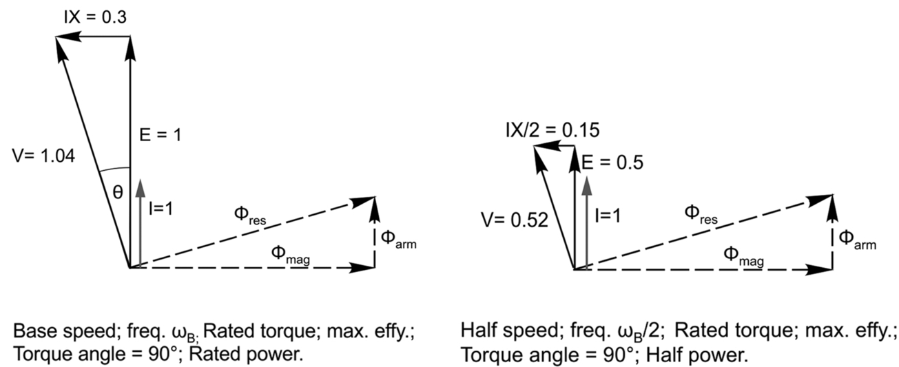
The magnet flux is the same as in Fig. 9.20 of course, and so for the same (rated) torque the stator current has to be 1 p.u., as before. However the frequency is now only half (ωB/2) so the open-circuit e.m.f. is now reduced to 0.5. The stator reactance is proportional to frequency, so it has also halved, to 0.15 p.u., and the volt-drop IX becomes 0.15 p.u. also. In view of the similarity between the diagrams it is no surprise that the applied voltage turns out to be half, i.e. 0.52 p.u., and given the emphasis we have previously placed on the fact that the flux in an a.c. machine is determined by the V/f ratio, we will not be surprised to see that this is again confirmed by these results.
The angle θ between V and I (the power-factor angle) is the same at full and half speed, and since the input power is given by VI cos θ, it is clear that the input power at half speed is half of that at full speed. This is what we would expect because with resistance neglected the input power equals the mechanical power, which is half in Fig. 9.21 because the torques are the same but the speed is half of that in Fig. 9.20.
The two previous examples have shown how the motor can be operated to produce full rated torque up to a speed at which the full available voltage is applied, i.e. this is what we have referred to previously as the ‘constant torque region’. In this region, the PM motor with field oriented control behaves, in the steady state, in a very similar manner to a dc motor drive, in that the applied voltage (and frequency) are proportional to the speed and the stator current is proportional to the torque.
We saw with the dc drive and the induction motor drive that once we had reached full voltage and current, any further increase in speed could only be achieved at the expense of a corresponding reduction in torque, because the input power was already at its maximum or rated value. In both cases, higher speeds were obtained by entering the aptly named ‘field weakening‘region.
For the dc motor, the field flux is under our direct control, so we reduce the current in the field circuit. In the induction motor, the field is determined indirectly by the V/f ratio, so if f increases while V remains constant, the field flux reduces. The PM motor behaves in a somewhat similar fashion to the induction motor, in that if the voltage is constant at speeds above base speed, the V/f ratio reduces as the frequency (speed) is increased, so the resultant flux also reduces. However, whereas the only source of excitation in the induction motor is the stator winding, the magnet in the PM motor remains a constant (and potent!) source of excitation at all times, and so we can anticipate that in order to arrive at a reduced flux to satisfy the V/f condition, the stator current will have to nullify some of the influence of the magnet. We must therefore expect less than ideal behaviour in the field-weakening region, which we now examine.
Field weakening—Operation at half torque, twice base speed (full power)
We will consider a situation well into the field weakening region, i.e. we will assume that in line with other drives we can expect full power, and so settle for operation at twice base speed and half rated torque. We will see that while this is achievable on an intermittent basis, it is not possible without exceeding the rated current, a conclusion that we must expect to apply to the whole of the field-weakening region with a PM drive.
The condition is represented by the phasor diagram shown on the right hand side of Fig. 9.22: the full load, base speed diagram is repeated on the left hand side to make comparison easy.

The frequency is twice the base value, i.e. 2ωB and so the open circuit e.m.f. is 2 p.u. As in other drives, above base speed we apply the maximum possible stator voltage, in this case 1.04 p.u. Because the voltage cannot be greater, it is not possible for us to arrange for the current to be in phase with E, and we are obliged to settle for a rather poor second-best.
The load torque is half rated, which means that the torque component of the current is 0.5 p.u. However, we note that the very large difference in voltage between E and V results in a very large stator volt-drop of IXs = 1.04 p.u. The reactance is twice as large as at base speed because the frequency is doubled, so the current is given by 1.04/0.6 = 1.74 p.u., which is 74% above its continuously rated value. The copper loss will therefore be increased by a factor of 1.742, i.e. to three times the rated value. Clearly continuous operation will not be possible because the stator will overheat, so in this field-weakening condition only intermittent operation at half torque will be possible.
By comparing the flux triangles in Fig. 9.22 we can see why the condition shown on the right side is referred to as field weakening. At base speed (the left hand figure) our freedom to adjust V allowed us to ensure that the stator or armature flux is in quadrature with the magnet flux (i.e. the torque angle λ is 90°), leading to a slightly higher resultant flux, and maximising efficiency by minimising the current for the given torque.
In contrast the constraint on V means that at twice base speed the armature flux has a large component which is in opposition to the magnet flux, leading to a resultant flux that is much less than the magnet flux, and a very low torque angle (λ) of only 16.8°. In a sense therefore, most of the stator current is ‘wasted’ in being used to oppose the magnet flux. Clearly this is not a desirable operating condition, but it is the best that we can get with the limited voltage at our disposal.
As a final check we can calculate the input power. The angle θ is given by 90°− 2λ = 56.4°, so the input power (VIcosθ) is 1.04 × 1.74 × 0.553 = 1 p.u., as expected since we assumed that the mechanical power was at rated value (twice base speed, half rated torque) and we ignored resistance in our calculations.
At this point we should recall that the aim throughout Section 9.5 has been to discover how the motor parameters determine the steady-state behaviour when the voltage, frequency and load vary over a range that is representative of a typical inverter-fed drive. Few readers will find it necessary to retain all of the detail (although a general awareness of the broad picture is always helpful) so those who have found it hard going can take comfort from the fact that in practice the drive will take care of everything for them. This is discussed in the next section.
9.6 Synchronous motor drives
Inverter fed operation of synchronous machines plays a very important and growing role in the overall drives market, as customers seek higher efficiency and higher power density than can be achieved with induction motors. We will see later, when we consider some of the available PM motor designs and control strategies, that very high dynamic performance can be achieved, making this the motor of choice in many of the most demanding applications.
9.6.1 Introduction
In Sections 9.4 and 9.5 we looked at the steady-state behaviour of the various types of synchronous motor when supplied with balanced sinusoidal voltages, and over a range of frequencies, when both voltage and frequency were independent of what was happening in the motor.
We saw that, as expected in a motor that has to compete with the induction motor, the synchronous motor has the inherent ability to accommodate to load changes: if the shaft load is increased, the rotor slows momentarily until the load angle and in-phase component of current have increased to produce more torque, and allow it to regain a new steady-state at the original speed. However, we also saw that under these ‘voltage fed’ conditions the maximum torque occurs when the load angle reaches 90°, and if it exceeds this value, the rotor will drop out of synchronism, the average motor torque will then be zero, and the motor will stall. It is easy to imagine that loss of synchronism may also occur if the frequency is increased too quickly: as the resultant field begins to accelerate, the load angle (between the resultant field and the rotor direct axis) initially increases, so the torque rises and the rotor begins to accelerate: but, depending on the inertia, if the load angle exceeds the point of maximum torque (90°), the rotor will ‘pole slip’, and stall. Loss of synchronism is clearly not acceptable for a general-purpose drive, which explains why early inverter-fed synchronous motor drives were not widely used.
Fortunately all the shortcomings of the utility-fed motor can be completely avoided by making the supply to the motor terminals respond almost instantaneously to what is happening inside the motor. As with the induction motor drive, this only became possible when fast digital processing could be harnessed to allow rapid control of the Inverter.
We will see that in these so-called ‘self-synchronous’ drives, the rotor is incapable of losing synchronism and stalling because the switching pattern of the inverter (and hence the frequency and speed) is determined by the rotor position and not by an external oscillator. We will also see that field oriented control can be readily applied to synchronous machines to achieve the highest levels of performance and efficiency with machines which have higher inherent power densities than the equivalent induction motors.
The reader may have noted that the stator current, which had been central to the discussion of torque production in Section 9.3, was relegated to being a dependent variable in Sections 9.4 and 9.5. This was because, having specified the voltage, frequency, and load, we had no direct control of the current, the magnitude and phase of which were obliged to assume the unique values that produced the required torque. In contrast, all of the drives that we look at in this chapter have current controllers at the heart of their torque control system, so we will see that current re-asserts its importance, and we will then be able to make use of many of the ideas relating to torque production that were introduced in Section 9.3. (We can continue to make use of the lessons we learned from the phasor diagrams in the previous sections, but they will only apply after the drive has reached a steady state in which the terminal voltage and frequency are constant.)
The reader will also be pleased to know that we will find many comforting similarities with d.c. and induction motor drives, but in relation to the sign of the torque, the synchronous machine is very different from the d.c. or induction motor. In the d.c. machine, the torque depends on the polarity of the armature current; in the induction motor the deciding factor is the whether the slip is positive or negative; but in the synchronous motor, it is the sign of the torque angle that matters, as shown in Fig. 9.23.
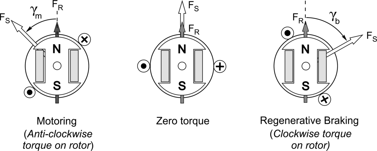
Fig. 9.23 shows in simplified form the rotor, the stator and rotor m.m.f. space waves (Fs and Fr, respectively), and the corresponding sinusoidally distributed stator current distribution (the latter being very crudely represented by a single-turn coil). The sketch is equally valid as a freeze-frame view of synchronous operation, when all of these elements are rotating anticlockwise at the synchronous speed (in which case the rotating stator current distribution is the resultant of three stationary windings with alternating currents) or with the machine at standstill with each (d.c.) phase current frozen at its appropriate value.
Recalling that the two m.m.f. waves always try to align themselves (or by applying ‘BIl’), we see that in the sketch on the left, the rotor torque is anticlockwise, because the stator m.m.f is displaced by a positive torque angle (γm) with respect to the rotor axis, while if the stator m.m.f. is to the right of the rotor axis the torque angle (γb) is negative and the torque on the rotor is clockwise. It should be clear that when the motor current (rather than the voltage) is the independent variable, the torque angle (between the stator and rotor m.m.f.'s) becomes of central interest, rather than the load angle.
Under running conditions, with the rotor turning anticlockwise, the left hand sketch represents motoring, the rotor lagging behind the stator m.m.f./flux wave, with energy being converted from electrical to mechanical form. Our concern in what follows will be to explain how we supply and control the magnitude and position of the stator current wave with respect to the rotor axis in order to achieve the desired torque. In most cases where full torque is required (for example during acceleration) the torque control system will supply each phase with rated current, and the torque angle will be maintained at or close to 90°, so that as the motor picks up speed, the period of each complete electrical cycle progressively reduces and the rotor therefore remains synchronised throughout.
We mentioned above that Fig. 9.23 applies equally when the motor is running at a steady speed, or is accelerating or decelerating, or is at rest, so it will probably be a helpful image to bear in mind for the remainder of this chapter.
We will now look at the power electronic converters and control strategies used with the various types of synchronous machine, and in the same order as in previous sections of this chapter. The last three all use pulse width modulated voltage source inverters (VSI), but the first - the excited rotor machine – is often supplied from a current source inverter (CSI) because the latter is better suited to the very high (multi-megawatt) power levels involved.
9.6.2 Excited rotor motor
Applications for this type of drive fall into two main categories.
Firstly, as a starting mechanism for very large synchronous machines, to bring them up to speed prior to synchronising to the utility supply, the converter then being rated for only a fraction of the machine rating. The main motor is started off load, synchronised to the utility supply and the load is then applied.
Secondly, as large high power (and sometimes high speed) variable speed drives for a variety of applications. Power ratings, typically from 2 to 100 MW at speeds up to 8000 rpm are available. At these high powers, it is advantageous to increase the operating voltage in order to minimise the current and thereby make the windings and interconnecting power cables more manageable: supply voltages up to 12 kV are typical, but systems over 25 kV are in service in which case the high voltage converter technology is similar to that used for HVDC power-system converters.
Some manufacturers of synchronous machines of much more modest ratings (e.g. a few tens of kW), also offer low voltage, thyristor based converter technologies, but they tend to be niche products.
The detailed design of high power drives, and the detailed consideration of the impact on the utility supply are beyond our scope, but we can cover the main principles without too much difficulty.
The power circuit and basic operation
The basic components of the high power, high voltage drive system are shown in Fig. 9.24.

The two fully-controlled converters are connected via a d.c. link that includes a large inductance to ensure continuous current operation. Current in the top of the d.c. link always flows from left to right, (as shown by the direction of the thyristors), but, as we saw in Chapter 2, the link voltage can be positive or negative (see below) so that energy can flow in either direction. The direction of rotation of the machine is determined electronically by the switching sequence within the machine converter, and hence full four-quadrant operation is available without extra hardware. The labels ‘rectifier’ and ‘inverter’ in Fig. 9.24 indicate how each converter operates when the machine is operating as a motor, their roles being reversed when the machine is braking or generating.
In view of what we have read so far, we might have expected the switching devices in the motor inverter to be IGBT's, and to see PWM control of the output voltage waveform, but in these large sizes, IGBT devices are expensive, and this explains why the motor converter is exactly like that used on the supply side of a d.c. motor drive.
The reason why we can use this cheaper inverter lies in the fact that, once rotating, a synchronous machine generates a.c. voltages in each phase winding that facilitate the commutation of a converter connected to its terminals. This is why it is frequently referred to as a Load Commutated Inverter (LCI). In effect the motor converter behaves in the same way as it does when connected to the utility supply.
There are close parallels between the combination of the motor side inverter and synchronous motor (enclosed by the dashed line in Fig. 9.24) and the conventional brushed d.c. motor, which explains why the combination is sometimes referred to as an ‘inside-out’ d.c. machine. We will explore the similarity, because we will then find it instructive to help us to understand how this particular drive operates.
In the synchronous motor the moving rotor carries the d.c. field winding. The rotating flux induces a sinusoidal e.m.f. in the three stator windings, the magnitude and frequency being proportional to the rotor speed and field current. The firing of the devices in the inverter is synchronised to these induced e.m.f.’s (and hence to the rotor position) so that the link current is fed sequentially into each phase at the optimum rotor angle to maximise torque, the inverter effectively acting as an ‘electronic commutator’. The d.c. link therefore ‘sees' a rectified 3-phase voltage that, although unidirectional, is not smooth d.c. (see Fig. 9.26): it can be thought of as the equivalent of the ‘back e.m.f.’ in a brushed d.c. motor.
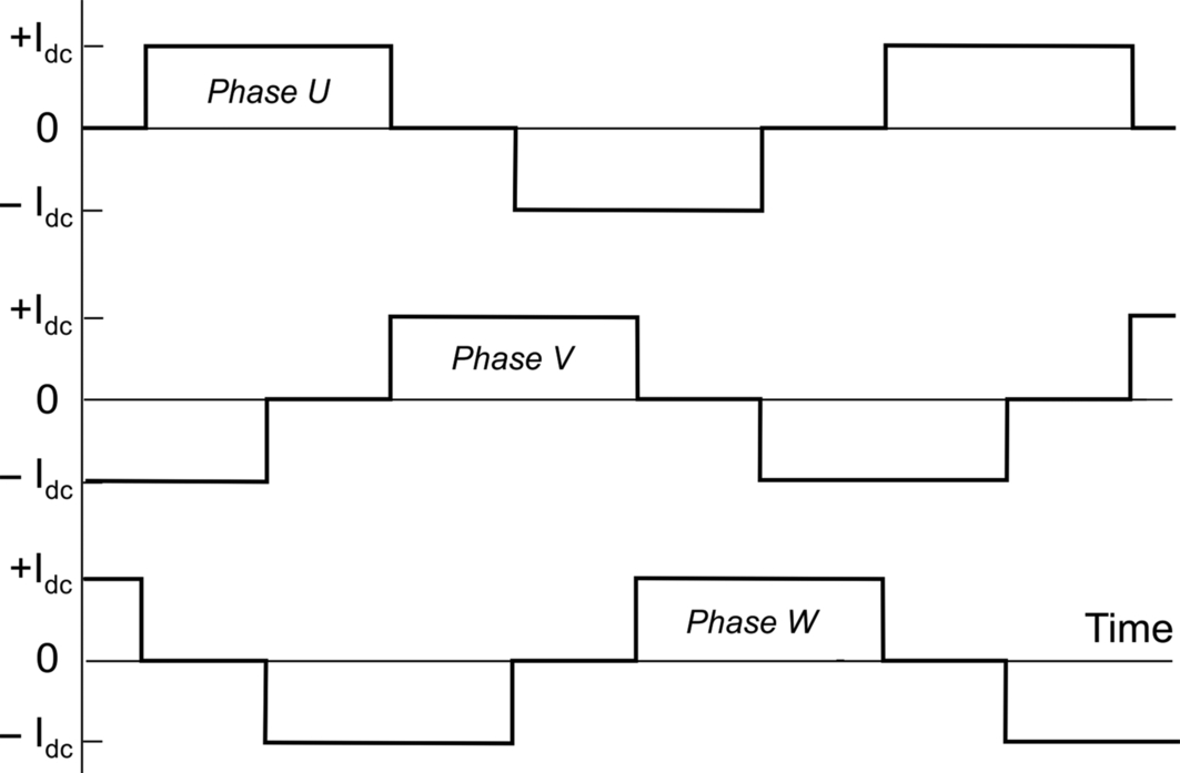
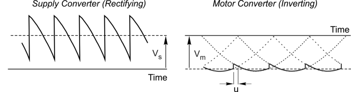
Conversely, in the conventional d.c. motor, the field is stationary, and its flux induces a motional alternating e.m.f. in the (many) armature coils on the rotor. The mechanical commutator and its sliding brushes rectify the e.m.f. so that at the armature terminals we get a very smooth d.c. induced voltage that we refer to as the back e.m.f, and denote by the symbol E.
So when viewed from the d.c. link, the two are essentially the same. It is therefore not surprising that, as with a d.c. motor, the no-load speed of the synchronous motor depends on the d.c. link voltage provided by the supply-side converter, while when load is applied and speed tends to fall, reducing the induced e.m.f., the d.c. link current automatically increases, thereby producing more torque until the steady-state is reached. The effects of varying the d.c. excitation on the rotor of the synchronous machine also mirror those in the d.c. motor, so that field weakening will lead to higher speed but reduced torque for a given link current.
Returning to the synchronous motor itself, and assuming that the link current is sensibly constant (see below), the switching strategy of the motor converter is synchronised to the induced e.m.f. of the machine and hence to the rotor position. In the steady state, each phase conducts the link current (Idc) for one third of a cycle of the generated e.m.f., i.e. 120o (elect); it is zero for the next 60°; and the pattern is repeated in the negative half-cycle, giving the current waveforms as shown in Fig. 9.25. (These are idealised waveforms, in which the d.c. current is assumed to be constant, and the current transitions from one value to another instantly, in the interest of simplicity: in practice there will of course be some current ripple and finite rise and fall times, the latter determined by the so-called ‘transient reactance’ of each phase, which fortunately is relatively low.)
If as is usual the windings are sinusoidally distributed, the resultant stator m.m.f. will always be sinusoidally distributed around the machine despite the non-sinusoidal current waveforms. But instead of progressing smoothly around the stator (as it would if the phase currents were sinusoidal in time), the m.m.f. jumps forward in space by 60° (elec) (i.e. one third of a pole-pitch) every time the motor converter commutates the link current to the incoming phase. Hence in the steady state there will inevitably be a torque ripple, which is the price to be paid for having a relatively unsophisticated inverter. Happily, resonances excited by the torque ripple are rare and can usually be overcome by preventing continuous operation at particular speeds associated with any mechanical resonance.
We have illustrated the basic operation by focusing on the steady-state, but it is important to remind ourselves that this is very different from the utility-fed case we looked at previously. In the utility-fed situation, the motor will lose synchronism and stall if the pull-out torque is exceeded. Here, the motor is self-synchronising, and if the load on the shaft is greater than the torque that can be developed when the link current is at its maximum, the motor will simply slow down, and pick up speed again when the shaft load is reduced, just as in a d.c. motor.
Current source inverter (CSI)
The term ‘Current Source Inverter’ has already been used to describe the power circuit shown in Fig. 9.24, so it is now time to explain what the term means.
It may be unnecessary, but we will start by making the point that the term current source inverter does not mean that the link current never changes, which is what a reader who is familiar with current sources in other contexts, especially in low power electronics, might think. In the present context, it means that under normal operating conditions, the link current cannot be changed rapidly, i.e. not significantly during one complete period of the motor current waveform, even at the lowest operating speed. The reader will not be surprised to learn that the link inductor is central to achieving this state of affairs.
We have said many times before in this book that inductance in a circuit results in the current waveform being much smoother than the voltage waveform (see for example Fig. 8.10), and that the bigger the inductance, the smoother the current. We need to recall that the voltage across an inductor is related to the current through it by the equation
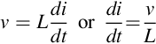
i.e. the rate of change of current is proportional to the voltage difference and inversely proportional to the inductance.
The rectified output voltage waveform of the supply-side rectifier will typically be as shown (left) in Fig. 9.26, which shows the potential of the top of the converter (i.e. at left hand end of the inductance) with respect to the bottom of the d.c. link. It a has a substantial ripple at six times the utility frequency, and the average (d.c.) voltage is (Vs).
At the same time the motor side converter (which is connected upside down) is inverting and the potential of the right hand end of the inductor will be as shown on the right of Fig. 9.26; the average (d.c.) voltage is (Vm). Note that whenever we want the link current to be constant, the first requirement is that the average voltage across the inductor is zero, which means that Vs must be equal to Vm, i.e. the d.c. voltage is the same for both converters. The current controller will adjust the firing angle of the supply-side rectifier in order to achieve this. (In practice there will be a small voltage difference because of the resistance of the inductor.)
The instantaneous voltage across the inductance is the difference between the two waveforms in Fig. 9.26. Finding the difference would be difficult because the two waveforms are not synchronised in time, but we can see that there will be substantial voltages across the inductor, not least the sudden step changes as a result of each supply converter commutation. If no inductance was present, there would consequently be huge step changes in the link current, and wild fluctuations in the motor torque. Hence we need to decide how much ‘ripple’ current we can tolerate, and choose the inductor accordingly. In practice a peak ripple of say 5% of rated current is typical for most applications.
Having chosen the inductor to suppress the current ripples, it is inevitable that when we want to raise or lower the mean current in order to vary the torque, the inductor will impede our efforts, and the response of the current control loop will be more sluggish. Fortunately, in large motors, we are not usually seeking high bandwidth torque control, so the compromise is acceptable.
The reason for the description ‘current source’ should now be clearer. Despite the switching of the link current from one phase to another in which the instantaneous induced e.m.f. is very different, the link current remains more or less unchanged, so that the impression we get is that the link current is independent of the load that we present to it.
Starting
So far we have assumed that the motor is running in the steady state, so that the motor terminal voltage (or better the back e.m.f.) can be used to determine the rotor position, but at start up and at very low speeds the magnitude of the back e.m.f. is too small to be used for control purposes or to commutate the current in the motor converter. The commutation is usually achieved by momentarily switching off the d.c. link current (by phase control of the utility side converter). When the current has reduced to zero the next pair of thyristors can be fired and the current built up again. A shaft mounted absolute position sensor provides position information to determine when the current should be commutated from one switch to the next. Whilst this sounds a slow and laborious process, it is not, and large machines can be accelerated in a few seconds. Above approximately 5% of rated speed the machine generates sufficient voltage for natural commutation, and subsequent control is undertaken in a similar manner to that of a d.c. drive.
Where the load is highly predictable some systems actually impose a pre-determined sequence of current pulses (applied sequentially to the motor phases) to “crank” the motor up to a speed at which the back e.m.f. becomes of sufficient magnitude to be used for position sensing and commutation. Such systems can avoid the need for a shaft mounted position sensor.
As in the d.c. drive, the a.c. supply power factor is poor at low speeds, but on the plus side, full four-quadrant operation is possible without any additional equipment.
Control
The fact that the synchronous motor/self-commutating thyristor converter combination behaves in much the same way as a conventional d.c. motor means that the control philosophy that we discussed in Chapter 5 can be employed, as shown in Fig. 9.27.

An inner current control loop provides torque control, and the torque reference is obtained from the error signal from the outer speed control loop. The maximum current is limited by clamping the current reference signal, Iref.
The items inside the chain-dotted line in Fig. 9.27 form the essential elements of a self-synchronous motor, and all that is necessary for it to function is a d.c. supply, shown as Vm in Fig. 9.27. The control scheme is the same as we saw for the conventional d.c. motor (Fig. 4.12), and it operates in much the same way as previously described, including field weakening, the rotor field current being reduced progressively as the link voltage gets close to its maximum value.
Looking back to Fig. 9.26, the frequency and amplitude of the motor-side voltage waveforms are of course proportional to the speed, and in motoring mode the converter firing angle delay is kept constant at slightly less than 180°, so that the torque angle is maintained at + 90°, thereby maximising the torque for the given current. The safety angle ‘u’ (see Fig. 9.26) is necessary to ensure successful commutation.
When regeneration is required, the firing angle delay of the motor converter is reduced to zero, the torque angle then becomes − 90° to give maximum braking torque and the motor converter then rectifies with maximum voltage (and hence maximum power and torque). Energy then flows back to the supply converter, which will have moved into the inverting mode in order to control the current to its demanded value.
Finally, we should note that current source inverters are now being challenged at powers up to 5 MW by voltage source inverters, the basic circuit and control of which is the same as for the PM motor to which we now turn.
9.6.3 Permanent magnet motor
Permanent magnet motor drives are a very important and rapidly growing sector of the drives market, and we will be looking in Section 9.7 at the excellent performance characteristics of these drives in more detail to explain why. In terms of the practical implementation, we have little new to introduce because the converter circuits used in commercial drives are exactly the same as we have already discussed in Chapters 7 and 8 for the induction motor, and the control is also very similar.
The power circuit
The general arrangement used in the control of PM motors (and all synchronous motors apart from the excited-rotor type) is as shown in Fig. 7.2.
The inverter bridge is shown in Fig. 9.28 (it is the same Fig. 2.21, but repeated here to avoid turning back).
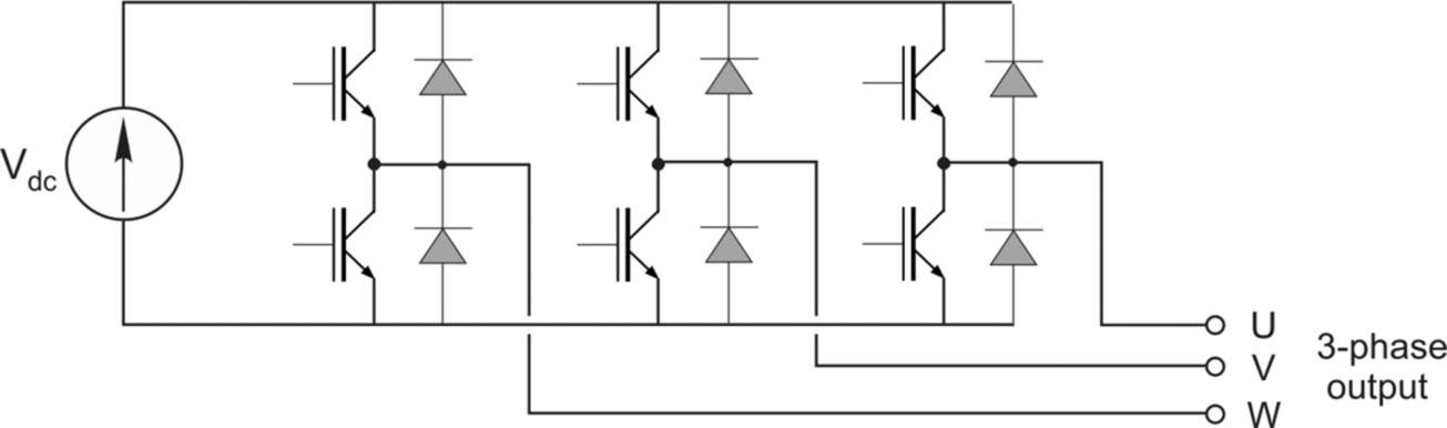
In Chapter 2 we discovered that during motoring operation (power flowing from the d.c. link to the motor) the power flows through the main power switch, usually an IGBT, and the reactive power flows through the anti-parallel diode. When the bridge feeds an induction motor, the magnetising (reactive) component of current is high, but in a PM motor there is no need for magnetising current when the motor is running below base speed, so there is the possibility of savings in terms of the diode rating, and also in improved inverter efficiency. We will consider the impact of operation above base speed (in the field weakening region) later.
Control
PM motors are almost always fed from a voltage source inverter, and so the control strategy is different from that for the current source inverter shown in Fig. 9.27. The arrangement of a typical field oriented control system for a PM motor is shown in Fig 9.29, in which the asterisk (⁎) is used to denote demanded quantities. As mentioned previously, the scheme is very similar to that for the induction motor (see Fig. 8.16).
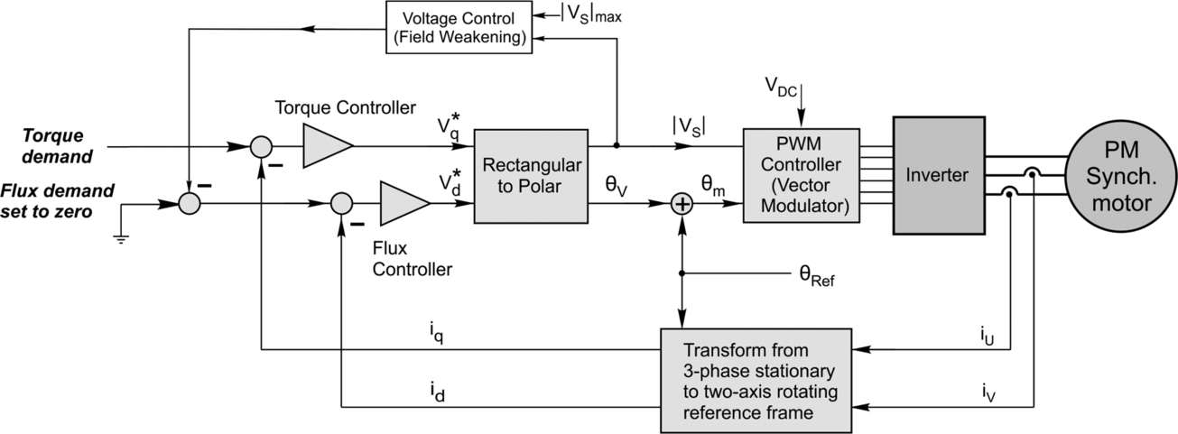
The flux demand has been set to zero because the flux is provided by the magnets. However, if the field current demand was not set to zero, the control system would provide a flux component of stator current that could either increase or decrease the effect of the magnet's flux, depending on the polarity of the reference signal. Clearly there will be an upper limit on the flux because of saturation of the magnetic circuit, and in practice, reducing the flux is a more attractive proposition because it allows us to operate in a field weakening mode and so extend the speed range into a constant power region, as discussed at the end of Section 9.5.
It would be possible to apply field weakening control by applying a speed-dependent term (− id), but this would require a good understanding of the machine characteristics, which is far from easy. A simpler approach can be applied if we think back to how we control a d.c. motor in field weakening (see Chapter 2). Steady-state operation up to base speed requires the stator voltage to increase with speed, but once base speed has been reached, the voltage, by definition, cannot increase any further. For the PM motor drive the situation is no different and so negative id must be imposed via the stator current, and a simple way to do this is shown by the additional “Voltage Control (Field Weakening)” loop at the top of Fig. 9.29.
Field weakening operation of PM motors presents an interesting practical problem that may occur if the control system should fail when running at high speed. For example, suppose the motor is running at three times base speed and for some reason the control system loses control. The component of stator current that is opposing the magnet flux disappears and so the rotor is spinning at three times base speed with full airgap flux, and the terminal voltage will rise to three times its rated value. The motor insulation systems and the power converter components are not normally rated to withstand such voltages and so catastrophic failure will result. Rating all components for such a situation would usually be cost prohibitive, and so other means of protection need to be sought. A common solution is to put a simple crowbar circuit near to the motor terminals, such that if such a fault does occur, and the terminal voltage rises, it is limited to an acceptable level.
9.6.4 Reluctance motor
The reluctance motor was once the motor of choice in the early days of power semiconductor based a.c. drives, but until recently had become all but forgotten, in a market dominated by the induction and PM motors. In recent years however, it has re-emerged as a commercial competitor of the induction motor. Whilst the motor is, in general, a little larger than the equivalent induction motor, some suppliers have put together credible motor/drive packages such as that shown in Fig 9.30.

The power circuit
The voltage source power converter (Fig 9.28) predominates for synchronous reluctance drives, and because it is common to induction motor and PM synchronous motor drives, a standard hardware platform can be utilised for the control of many different forms of a.c. motor. It turns out that the control strategy for the reluctance motor also has much in common with the induction and PM drives, as we will now see.
Control
Whilst reluctance motors can be operated with very simple control strategies, field orientation control is used in most commercial drives. We have seen in section 9.3.3 that as long as we are able to control the angle of the stator current phasor in relation to the rotor saliency we are able to directly control the motor torque. We have also seen that the torque depends on the square of the current, and that it is a double frequency function of the rotor angle.
The rotor design and modelling of reluctance motors has received a great deal of academic and industrial attention in recent years and the optimisation of the stator current phasor angle, taking into account the effects of saturation, is a subject area which is well beyond the scope of this book. To simplify matters, we will introduce an undefined ‘Current References’ function block into the control diagram, Fig. 9.31. In practice, the reality in many cases is that the function simply creates a fixed ratio of iq/id to give an angle close to the 45° associated with the peak torque as shown in Fig 9.8.

9.6.5 Salient permanent magnet motor
Control of the Salient PM (“PM/Rel”) motor is undertaken in much the same way as described above for the reluctance motor, but with more complex algorithms in the “Current References” box. Again relatively simple implementations based on a fixed ratio of Iq/Id are possible, but for optimised control, the impact of saturation, common in such machines, needs to be taken into account.
9.7 Performance of permanent magnet motors
Throughout this section we will use the terms ‘brushless’ and ‘permanent magnet’ to be synonymous when they are applied to an electric motor. We will also avoid the confusing term ‘brushless d.c. motor’ because, as already mentioned in the introduction, such motors are always supplied with alternating currents.
However we should mention that the inherent electromagnetic properties of a PM motor can be quantified by its ‘motor constant’ in much the same way as a d.c. motor (Chapter 3). If we spin the rotor of a PM machine at angular velocity ω, the r.m.s. value of the sinusoidal e.m.f. induced in each phase is given by E = kω, and if we supply balanced currents of r.m.s value Ia to the three phase windings in quadrature to the field, the torque is given by T = kIa, where k is the machine constant, expressed in the SI units of Volts per radian per second or the equivalent Newton-metres per Ampere. (In practice, manufacturers usually quote k in terms of Volts per thousand revs per min.) These relationships are identical to those we discussed earlier for the DC machine, and once again they underline the unity of machines that operate on the ‘BIl’ principle.
We have hinted previously that PM motors offer outstanding performance in terms of power density and performance in comparison with induction and d.c. machines, and in this section we look briefly at the underlying reasons. We then discuss the limitations that govern performance and finally give an example that illustrates the impressive results that can be obtained.
9.7.1 Advantages of PM motors
The stator windings of PM motors do not have to carry the excitation or magnetising current required by the induction motor, so a given winding can carry a higher work current without generating more heat, thereby increasing the electric loading and the specific power output (as discussed in Chapter 1).
Cooling the rotor is difficult in any enclosed machine because ultimately the heat has to get to the stator, so the absence of current on the rotor not only improves efficiency by reducing the total copper loss, but also eases the cooling problem.
Historically, brushless PM motors only became practicable with the advent of power electronics, so it became normal for them to be supplied via power electronics with the associated expectation that they would operate in a speed-controlled drive. The majority were therefore not expected to operate directly off the utility supply, and as a result their designers had much greater freedom to produce bespoke designs, tailored to a specific purpose. (The designers were also less hamstrung by standards developed over many years dictating shaft size and height, mounting arrangements and cooling arrangements.)
For example suppose we require a motor that can accelerate very quickly, which implies that the ratio of torque to inertia should be maximised. We saw in Chapter 1 that with given values of the specific magnetic and electric loadings, the torque is broadly dependent on the volume of the rotor, so we are free to choose long and thin or short and fat. The inertia of a homogeneous rotor is proportional to the fourth power of its radius, so clearly for this application we want to minimise the rotor radius, so a long thin design is required. Fortunately, there is considerable flexibility in regard to the shape and size of the rotor magnets, so no serious constraint applies in relation to rotor diameter. Many so-called servo motors have this profile, as illustrated in Fig. 9.32.
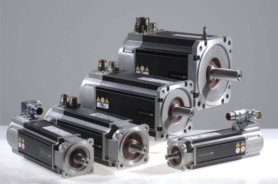
A different application with the same continuous torque and power requirements would require the same rotor volume, but if, for example, the application requires that unwanted changes in speed caused by step changes in load torque must be minimised, the inertia should clearly be maximised, with a short rotor of larger diameter.
A section through a high inertia PM motor typically rated up to 100 Nm and 3000 rev/min is shown in Fig. 9.33. It is interesting to note how little of the volume of the motor is actually taken up with active material, namely the stator and rotor laminations and the surface-mounted magnets on the rotor. The end windings of the stator windings are seen to contribute significantly to the overall volume of the motor illustrated. (The move to using segmented stator windings reduces the impact of the end winding and can lead to significant reductions in total motor volume.) Most PM motors employ rare-earth magnets which have much higher energy product (in effect a measure of their magnetising ‘power’) than traditional materials such as Alnico, so they are very small, as shown in Fig. 9.33.
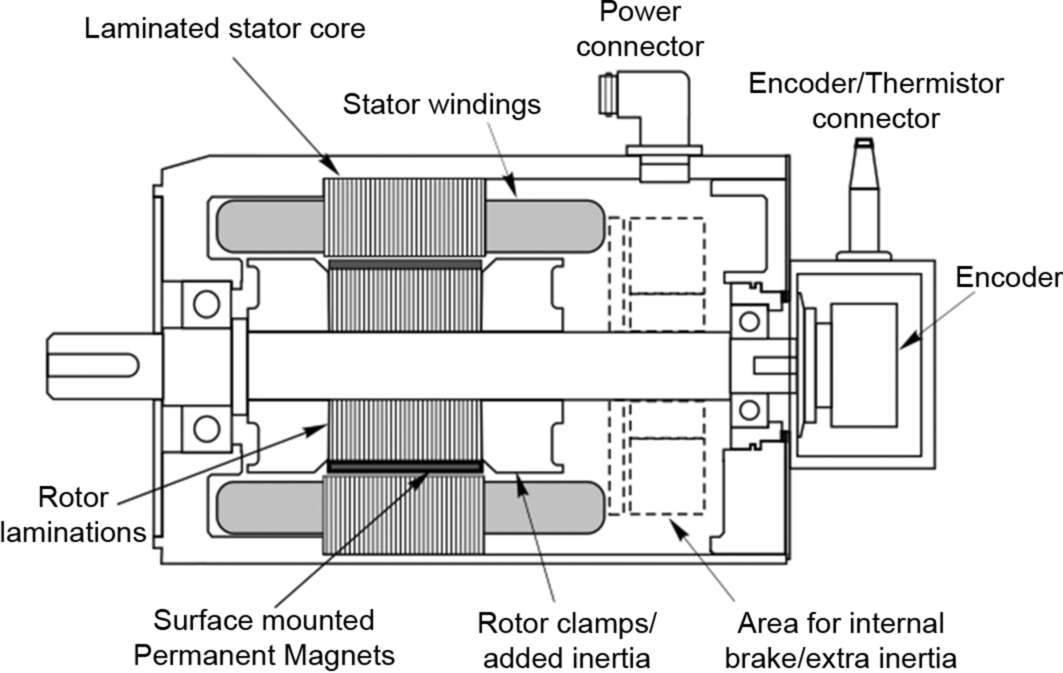
As in other motors the heat dissipated in the stator diffuses into the air through the frame to the finned case and hence to the surrounding air. However, the design of some motors of this type is based on the requirement that a substantial proportion (perhaps 40%) of the loss is conducted through the mounting flange to a suitable heatsink, so this is an area where great care needs to be taken with the thermal properties of the mounting.
9.7.2 Industrial PM motors
In the preceding section we mentioned that bespoke design of PM motors has long been considered unexceptional, but recent years have seen the emergence of PM motors packaged in the same industrial motor (IEC or NEMA) housings that are been used for induction motors, as shown in Fig. 9.34.

This type of motor is now marketed as a direct competitor of the induction motor in variable speed applications. They are targeted at general applications where the higher initial cost is offset by their higher efficiency and high power density. The heat loss in the permanent magnet rotor is much less than in the corresponding induction motor, so the rotor runs cooler which may also be an advantage in aspects such as bearing life.
9.7.3 Summary of performance characteristics
Permanent magnet motors with low inertia rotors are used in high performance servo applications such as machine tools or pick and place applications where fast precise movements are required, and motors with high inertia rotors (and high pole numbers) suit low speed applications such as gearless lift systems.
The performance characteristics of these drives are summarised below:
- • Excellent dynamic performance at speeds down to standstill when position feedback is used.
- • For precision positioning the position feedback must define the absolute position uniquely within an electrical revolution of the motor. This can be provided with a position sensor or alternatively a sensorless scheme can be used. The performance of a sensorless scheme will be lower than when a position sensor is used.
- • Field weakening of permanent magnet motors is possible to extend their speed range, but (as shown in Section 9.5) this requires additional motor current, and so the motor becomes less efficient in the field weakening range. This form of control also increases the rotor losses and raises the temperature of the magnet material, thereby increasing the risk of demagnetisation. Care is also needed in such applications to avoid overvoltage at the motor and drive terminals in the event of a loss of control: at high speeds, the open-circuit voltage will exceed the rated value.
- • Permanent magnet motors exhibit an effect called cogging that results in torque ripple. It is caused by magnetic reluctance forces acting mainly in the teeth of the stator, and can be minimised by good motor design, but can still be a problem in sensitive applications.
- • Permanent magnet motors can be very efficient as the rotor losses are very small.
To give an impression of the outstanding performance that can be achieved by a brushless PM motor, Fig. 9.35 shows the results from a bench test in which the speed reference begins with a linear ramp from zero to 6000 rev/min in 0.06 s, followed shortly by a demand for the speed to reverse to 6000 rev/min, then back to full forward speed and finally to rest, the whole process lasting less than 1 s.

The motor was coupled to a high-inertia load of 78 times the rotor inertia, which makes the fact that the speed reversal is accomplished in only 120 ms even more remarkable. It takes only three revolutions to come to rest and a further three to accelerate in reverse. In common with many high performance applications, the drive control is actually implemented in the form of position control, with the shaft angle being incremented at a rate equivalent to the required speed. The dotted trace in Fig. 9.35 shows the position error of the motor shaft throughout the speed reversal. The maximum error is less than 0.05o, so by any standard this is truly impressive. It is no wonder that the brushless PM motor is frequently chosen for applications where closely co-ordinated motion control is called for.
Finally, on a matter of terminology, it is worth pointing out that brushless PM motors are sometimes referred to as ‘servo’ motors. The name “servo” originates from ‘servomechanism’, defined as a mechanical or electrical system for control of speed or position. The term tends to be used loosely, but broadly speaking when it is applied to a motor it implies superior levels of performance.
9.7.4 Limits of operation of a brushless PM motor
We have previously talked about the limits of operation that determine the rating and operating envelope of other types of electrical machine, so we will conclude this section by taking a closer look at the limits of operation for a Brushless PM servo motor (which usually has no external cooling fins or fan). A typical torque-speed characteristic is shown in Fig. 9.36.
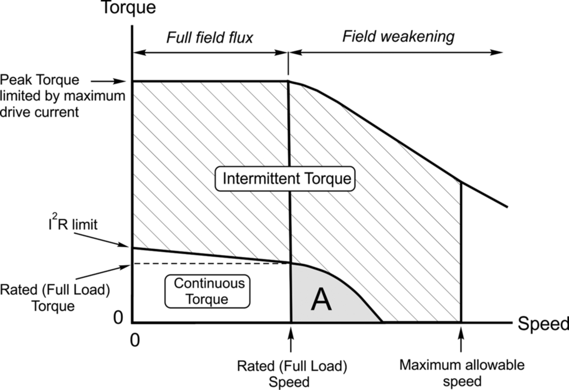
The individual limits shown in Fig. 9.36 are discussed below, but the most striking feature is clearly the very large area where operation above rated torque is possible (albeit on an intermittent basis). This provision clearly reflects the potential application areas, such as rapid positioning systems, where high acceleration is needed for relatively short periods.
The continuously-rated region is, as usual, limited by the allowable temperature rise of the motor. At standstill the predominant source of loss is the stator copper loss (shown as I2R limit in Fig. 9.36), but at higher speeds the iron loss becomes significant and the full load torque at rated speed is therefore less than the standstill torque.
The upper boundary of the intermittent torque region is usually determined by the maximum current that the drive converter can supply: only intermittent operation is possible otherwise the motor overheats.
Continuous operation is not possible when field weakening either, because, as explained in Section 9.5, the stator current is large in order to oppose the magnet flux. For this thermal reason Region A shown in Fig. 9.36 can be somewhat truncated compared with the characteristic field weakening region of the induction motor.
Operation of PM motors at excessive temperatures can lead to demagnetisation of the rare earth magnets in the motor, as well as the hazards common to all other electrical machine such as degradation of insulation. Good thermal protection is therefore necessary. Below base speed, for applications involving few excursions outside the continuous operating region, a relatively simple motor thermal model in the drive control scheme, may be adequate. For applications involving significant operation in the intermittent torque region, and certainly where field weakening operation is used, more complex thermal models would be needed and these are usually supplemented by thermistors embedded in the stator windings.
9.7.5 Brushless PM generators
As with almost all forms of electrical machines the PM motor can be operated as a generator, with mechanical energy supplied to the shaft being converted to electrical energy. The advantages of high power density and efficiency offered by the PM motor, of course apply equally when the machine is being used as a generator.
Many commercial wind generators up to 75 kW use PM synchronous machines. Much larger wind generators are also in service with some multi-pole multi-MW motors being applied in utility scale turbines with direct drive systems, i.e. systems which do not employ a gearbox between the wind turbine and the generator.
9.8 Emerging developments in permanent magnet motors
So far in the book, our discussions of a.c. machines (both induction and permanent magnet) have concentrated on machines with low pole-numbers (e.g. 2, 4, 6….), because they are by far the most numerous. The corresponding speeds when fed from the 50 or 60 Hz utility supplies cover the range from 1500 rev/min at 50 Hz to 3600 rev/min at 60 Hz, and are therefore well-suited to the majority of industrial applications.
We have also seen that for motors with similar magnetic and electric loadings, and similar cooling arrangements, the specific power output is proportional to the speed. A 4-pole, 50 Hz, 1500 rev/min, totally enclosed fan ventilated induction motor is therefore smaller than a 12-pole, 50 Hz, 500 rev/min version producing the same power output.
The availability of inverters that are highly efficient at frequencies in the kHz range has largely removed the frequency constraint, so that, regardless of pole number, the synchronous speed can now be varied smoothly up to much higher frequencies than that of the utility supply, so it is no longer necessary to have a low pole number to achieve the high speed required for a high specific output.
Superficially, the high pole-number stator windings of recently developed PM motors (see Fig. 9.39) often appear radically different from their predecessors, so we might expect to need a new approach in order to explain how they work. In fact, we will see that their novel stator windings represent limiting versions of the conventional multi-slotted, 2-layer stator windings, with coils spanning several slots (see Chapter 5), which means that their behaviour can be explained using the same ideas as we have used previously.
9.8.1 Advantages of high pole number
For a PM motor, where the main excitation flux is produced by magnets on the rotor, a higher pole-number brings advantages in terms of economy of copper and iron, and often simplicity of manufacture, and comparatively few disadvantages, as we will see shortly. This explains why higher pole numbers now predominate in PM motors, particularly those aimed at high-volume emerging markets such as electric vehicle drives, where investment in mass production is justified. (By contrast, it is worth pointing out that when the excitation is provided by the stator winding, as in an induction motor, a higher pole numbers is not inherently desirable (apart from yielding a low speed at 50 or 60 Hz). This is because to achieve a given magnetic loading the magnetising m.m.f. per pole must remain the same, but the available slot space per pole reduces as the pole number increases. Hence the proportion of the slot space to be devoted to the magnetising function increases, leaving less for the useful or work component of current. Induction motors with high pole numbers therefore have an unattractive low power factor.)
We are discussing permanent magnet (PM) motors, where the main flux is provided by the rotor magnets, so (as explained in Section 9.3) we now choose to picture torque production as the result of the magnet flux interacting with the currents on the stator, rather than stator flux interacting with rotor current. Thus when we refer to electric loading (see Section 1.5.1), we are referring to the stator, rather than the rotor.
The first and most obvious advantage of a high pole number (as compared with say a 2-pole) is that, for a given magnetic loading, the flux per pole is less and consequently the depth of iron core behind the slots (necessary to carry the circumferential flux from north pole back to south pole without saturating) is reduced. This results in a cost saving in expensive core steel on both stator and rotor, the latter being annular: a sketch showing 2-pole and 8-pole stators for the same rotor diameter, and similar magnetic loadings, is shown diagrammatically in Fig. 9.37.
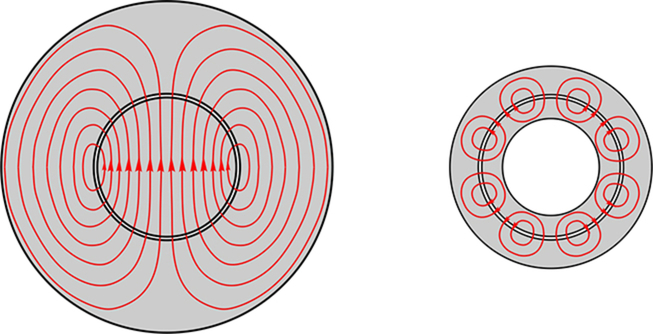
The second advantage relates to the progressive reduction in the length of the end windings as the pole number is increased. The function of the end windings is simply to connect the ‘go’ and ‘return’ sides of the coils: they contribute nothing to the output power, but their resistance represents a source of unwanted ‘copper loss’, so there are savings in both materials and losses when the pole number is increased.
9.8.2 Segmented core and concentrated windings
For high pole-number stators, splitting the stator core into segments has obvious attractions both in terms of automated coil assembly and reduction of waste in comparison with conventional (full circle) laminations: a typical set of interlocking segments is shown in Fig. 9.38.


Single-tooth versions that are pre-wound before assembly are now in widespread use for PM motors. They can have a relatively high fill factor, but the disadvantage of this ‘concentrated coil’ winding is that there is no longer any freedom (as there is with a 2-layer winding) to select the coil-pitch: in a concentrated winding spanning one tooth only, the coil pitch is of necessity equal to the slot pitch. We will see in the example in the next section that this leads to a relatively poor m.m.f. waveform.
9.8.3 Fractional slot windings
In order to understand how multi-pole stator windings with few slots derive from their conventional predecessors, we must briefly recap and then extend the discussion of fractional slot windings in Section 5.2.3. Readers who want to skip this detail will doubtless be happy to accept that it is not essential to understanding the remainder of the chapter.
Historically, the majority of a.c. machines (synchronous and induction) had stators with a large number of slots with 3-phase, 2-layer windings of the type discussed in Section 5.2 of Chapter 5. (By ‘a large number of slots’ we mean a range from perhaps 24 to around 100). This type of winding remains dominant, especially in the larger sizes.
In Section 5.2, we emphasised that conventional stator windings were laid out in order to produce a sinusoidal rotating magnetic field of a particular pole number. It became clear that by using a two-layer winding with coil pitch less than one pole-pitch, and with several slots per pole per phase (s/p/p), a set of identical coils could be distributed so that the resultant space wave of m.m.f. was a very close approximation to a sinewave, thereby minimising the undesirable effects of harmonic fields.
However, even with a large number of slots, there are occasions where the s/p/p is not an integer, for example a 4-pole, 3-phase, two-layer winding in a stator with 54 slots, for which the s/p/p = 4.5. Where the s/p/p is not an integer, the winding is described as ‘fractional slot’, and in such windings, some phase bands occupy more slots than others: in the example above, the first and third phase bands will occupy four adjacent slots, while the second and fourth will occupy 5 adjacent slots. As usual, all three phases will be identical but displaced by one third of a pole-pitch. Such windings have long proved to be entirely satisfactory.
Example: 10-pole, 3-phase winding in 12 slots
Returning for a moment to the 2-layer winding, we can see by comparing Figs. 5.4 and 5.3 that when the s/p/p reduces from 3 to 1, the m.m.f. waveform degenerates from a reasonable approximation to sinewave to a rectangular waveform, which is of course heavily polluted with harmonics. Many contemporary permanent magnet motor stators with concentrated windings take the move towards fewer slots per pole well beyond that shown in Fig. 5.3, and typically have values of s/p/p less than one. For example, for the 3-phase, 10-pole winding in 12 slots shown in Fig. 9.39, the s/p/p = 0.4.
The rotor in Fig. 9.39 clearly has 10 permanent magnets, which immediately indicates that it is a 10-pole machine. However, it is by no means self-evident (even to an experienced observer) that the 12-slot stator winding, fed with balanced 3-phase currents, will produce a 10-pole rotating field. (Indeed, given only the stator to examine, it would not be at all surprising if a non-expert concluded that it was for a 12-pole machine, or a switched reluctance motor, or a stepping motor (see Chapter 10).
To see that the winding will indeed produce a 10-pole field to cooperate with the rotor, we must examine the stator m.m.f., using the approach followed in Chapter 5.
Given that the aim of each phase winding is to produce a 10-pole m.m.f., the fact that there are only 4 slots for each phase clearly indicates that the outcome will inevitably be less than ideal. In fact, by sharing some of the slots with a coil from another phase (see Fig. 9.39), we manage to obtain 8 ‘half height steps’ in the phase m.m.f. waveform, as shown in Fig. 9.40: in this figure, the current in phase U is at a positive maximum, while each of the other two phases carry a negative current of half peak amplitude. The phase m.m.f. is clearly a very poor approximation to a 10-pole sinusoid, it probably being best described as a 10-pole square wave with six of the ten poles missing.

The other two phase-windings are identical to phase U, but displaced in space by 120° and 240° electrical (i.e. with respect to the 10-pole wave), and when their m.m.f.’s are added the resulting m.m.f. wave is much better, as shown by the resultant waveform in Fig. 9.40.
This example illustrates the extent to which expediency and cost of manufacturing outweigh considerations of purity of m.m.f. waveform for applications such as hybrid vehicles, where the motor will probably be integrated within the power train and cooled by engine oil. ‘Fault tolerance’ is at a premium in such duties, meaning that the motor is expected to continue to produce torque despite failure of one or more of its parts. In the case of the motor in Fig. 9.39, the four coils in each phase may be supplied from separate inverters, so that healthy coils can continue in the event of a failure elsewhere.
9.9 Review questions
- (1) What voltage should be used to allow a 420 V, 60 Hz, 4-pole synchronous motor to be used on a 50 Hz supply?
- (2) What purpose, might be served by a pair of 3-phase synchronous machines (one of which has ten polar projections on its rotor and the other twelve) mounted on a bedplate with their shafts coupled together, but with no shaft projections at their outer ends?
- (3) The book explains that in excited-rotor synchronous machines the field winding can be supplied with d.c. current via sliprings. Given that the field winding rotates, why is there no mention of any motional e.m.f. in the rotor circuit?
- (4) A large synchronous motor is running without any load on its shaft, and it is found that when the d.c. excitation on the rotor is set to either maximum or minimum, the a.c. current in the stator is large, but that at an intermediate level the stator current becomes almost zero. The stator power seems to remain low regardless of the rotor current.
Explain these observations by reference to the equivalent circuit and phasor diagram. Under what conditions does the motor look like a capacitor when viewed from the supply side? - (5) This question refers to Fig. 9.5. In the motor shown on the right of Fig. 9.5, what would happen if the polarity of the stator current was suddenly reversed?
- (6) How many discrete stable equilibrium positions would you expect to find in a 4-pole reluctance motor? (Hint: imagine the stator current to be d.c. as in the 2-pole example in Fig. 9.8.)
- (7) By clever re-design of the rotor of a current-fed reluctance motor, the quadrature axis reactance is reduced while the direct axis reactance is unchanged, and as a result the ratio of direct to quadrature reactance is increased from 4 to 5. If the motor is current-fed, by how much will the peak torque increase?
- (8) The stator of a 10-pole PM motor is supplied with a steady (d.c.) current from a battery, and the unloaded rotor is at rest at an angle of 0°.
- (i) The rotor is then turned by hand before being released. At what angle will the rotor eventually come to rest if the angle it is initially turned through is (a) 15°, (b) 45°.
- (ii) At what angle(s) will the maximum torque be detected?
- (iii) If the polarity of the current is reversed, at what angle will the rotor settle?
- (9) Explain briefly why, for a PM motor, it is possible for a given torque to be produced for a range of values of stator current.
- (10) A PM motor driven from a voltage source inverter is running light at its base speed and the current is negligible. The speed is increased to twice base speed, and despite having no load on the shaft, the current is now much larger. Explain, preferably with the aid of phasor diagrams.
Answers to the review questions are given in Appendix.