Motor/drive selection
Abstract
The availability, ratings, speeds, and main characteristics of the various drives are presented in convenient tabular form. We then discuss the principal factors involved in drawing up a specification, including the nature of the load; duty cycle; supply system effects; and prevailing standards.
Keywords
Motor/drive selection; Load types; Torque-speed; Power ratings; Performance; Advantages; Disadvantages; Duty cycle
11.1 Introduction
The selection process often highlights difficulties in three areas. Firstly, as we have discovered in the preceding chapters, there is a good deal of overlap between the characteristics of the major types of motor and drive. This makes it impossible to lay down a set of hard and fast rules to guide the user straight to the best solution for a particular application. Secondly, users tend to underestimate the importance of starting with a comprehensive specification of what they really want, and they seldom realise how much weight attaches to such things as the steady-state torque-speed curve, the dynamic performance required, the inertia of the load, the pattern of operation (continuous or intermittent), the environment and the question of whether or not the drive needs to be capable of regeneration. And thirdly they may be unaware of the existence of standards and legislation, and hence can be baffled by questions from any potential supplier.
The aim in this chapter is to assist the user in taking the first steps by giving some of these matters an airing. We begin by laying out the availability, ratings and speeds, and then the main characteristics of the various motor and drive types that we have highlighted earlier in the book. We then move on to the questions which need to be asked about the load and pattern of operation, and finally look briefly at the matter of standards. The whole business of selection is so broad that it really warrants a book to itself, but the cursory treatment here should at least help the user to specify the drive rating and arrive at a short-list of possibilities.
11.2 Power ratings and capabilities
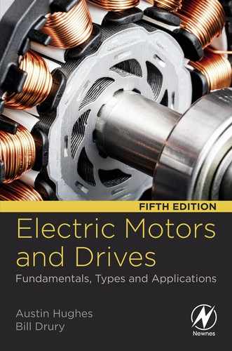
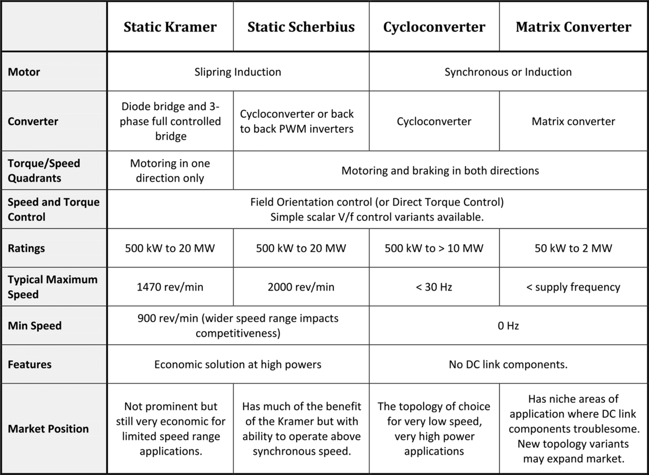
The four tables in this section represent an attempt to condense the most important aspects that will be of interest to the user into a readily accessible form. It will be evident from the weight given to a.c. drives in the book that they now dominate the scene, and this is reflected in the fact that only the first table deals with d.c. drives. The scope of a.c. drives is too great for a single table, so to aid digestion we have split them into three.
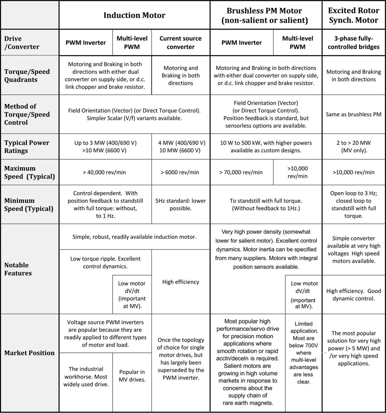
The first table (Fig. 11.1) covers conventional (brushed) d.c. motor drives, which remain significant despite their diminishing market share. However, the second table (Fig. 11.2—a.c. drives) is by far the most important because it includes the inverter-fed induction motor and brushless PM motor drives which are now the most widely used industrial drives. The (synchronous) reluctance motor is not separately identified here but can be considered as an alternative to the induction motor in most applications (though the motor tends to be a little larger). The emergence of the salient PM synchronous machine in recent years is having a growing impact in many markets including automotive traction: its operational characteristics closely follow those of the nonsalient PM motor and for this reason they have been discussed together in this summary. Fig. 11.3 deals with (predominantly large) a.c. drives, which have limited and/or niche application and are therefore less common: for completeness the static Scherbius drive is included although it was not discussed. The fourth table (Fig. 11.4) contains three unlikely bedfellows whose conjunction reflects the fact that they could not be fitted in elsewhere.


11.3 Drive characteristics
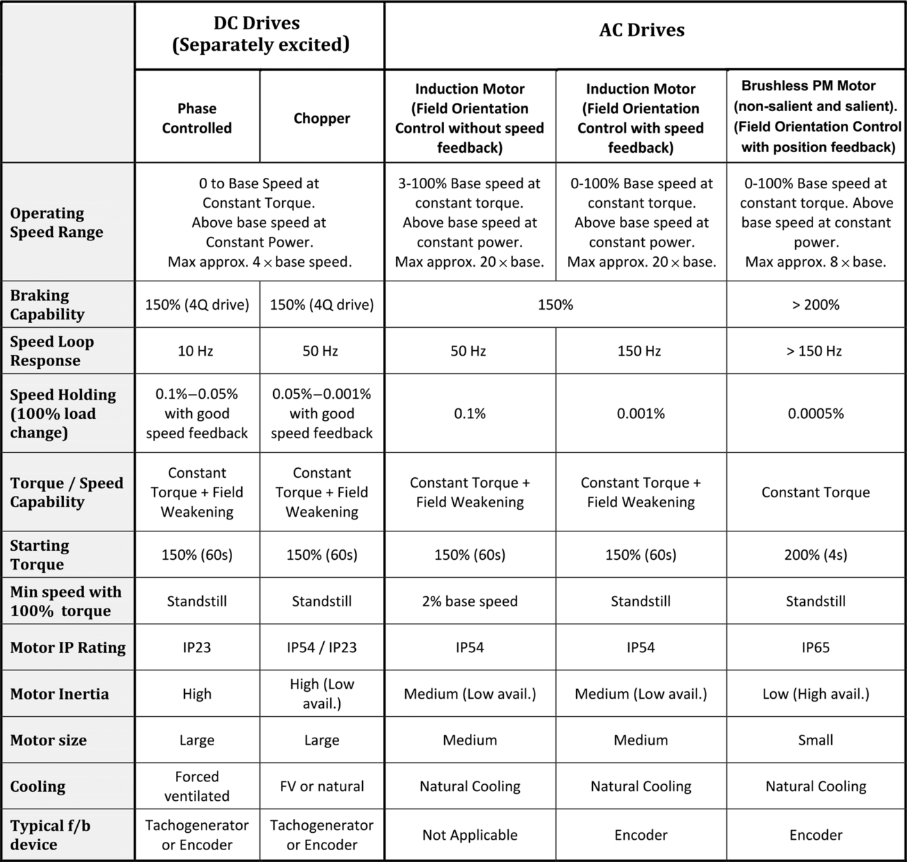
The successful integration of electronic variable speed drives into a system depends on knowledge of the key characteristics of the application and the site where the system will be used. The correct drive also has to be selected, but this is often simpler than it used to be because the voltage source PWM inverter has become universally adopted for almost all applications, and its control characteristics can be adapted to suit most loads with relative ease. It is still important to understand the general characteristics of the various types of drive, however, and these are listed in summary form in the table (Fig. 11.5). (Note that the data on overloads relates to typical industrial equipment, but users will inevitably encounter a range of different figures from the various suppliers.) Finally, a summary of the pros and cons of d.c. and a.c. drives is given in the table (Fig. 11.6). The wealth of information in these tables should be of great value in assisting prospective users to narrow down their options.

11.3.1 Maximum speed and speed range
This is an important consideration in many drives, so a few words are appropriate. We saw in Chapter 1 that as a general rule, for a given power the higher the base speed the smaller the motor. In practice there are only a few applications where motors with base speeds below a few hundred rev/min are attractive, and it is usually best to obtain low ‘maximum’ speeds by means of mechanical speed reduction often in the form of a gearbox.
Motors speeds above 10,000 rev/min are also unusual except in small universal motors and special-purpose inverter-fed motors for applications such as aluminium machining. The majority of motors have base speeds between 1500 and 3000 rev/min: this range is attractive as far as motor design is concerned since acceptable power/weight ratios are obtained, and these speeds are also satisfactory as far as mechanical transmission is concerned. Note, however, that as explained in Chapter 1, the higher the rated speed the more compact the motor, so there will be instances where a high speed motor is preferred when minimising motor size is of paramount importance.
In controlled-speed applications, the range over which the steady-state speed must be controlled, the required torque/speed characteristic, the duty cycle and the accuracy of the speed-holding, are significant factors in the selection process. In Chapter 7, we looked at some of these aspects, notably in relation to motor cooling. For constant torque loads which require operation at all speeds, the inverter-fed induction motor, the inverter-fed synchronous machine and the d.c. drive are possibilities, but only the d.c. drive would come as standard with a force-ventilated motor capable of continuous operation with full torque at very low speeds.
Fan or Pump type loads (see below), with a wide operating speed range, are a somewhat easier proposition because the torque is low at low speeds. In most circumstances, the inverter-fed induction motor (using a standard motor) is the natural choice.
Figures for accuracy of speed holding can sometimes cause confusion, as they are usually given as a percentage of the base speed. Hence with a drive claiming a decent speed holding accuracy of 0.2% and a base speed of 2000 rev/min, the user can expect the actual speed to be between 1996 rev/min and 2004 rev/min when the speed reference is 2000 rev/min. But if the speed reference is set for 100 rev/min, the actual speed can be anywhere between 96 rev/min and 104 rev/min, and still be within the specification.
11.4 Load requirements—torque-speed characteristics
The most important things we need to know about the load are the steady-state torque-speed characteristic, the effective inertia as seen by the motor and what dynamic performance is required. At one extreme, for example in a steel rolling mill, it may be necessary for the speed to be set at any value over a wide range, and for the mill to react very quickly when a new target speed is demanded. Having reached the set speed, it may be essential that it is held very precisely even when subjected to sudden load changes. At the other extreme, for example a large ventilating fan, the range of set speed may be quite limited (perhaps from 80% to 100%); it may not be important to hold the set speed very precisely; and the times taken to change speeds, or to run-up from rest, are unlikely to be critical.
At full speed both of these examples may demand the same power, and at first sight might therefore be satisfied by the same drive system. But the ventilating fan is obviously an easier proposition, and it would be overkill to use the same system for both. The rolling mill would call for a regenerative drive with speed or position feedback, while the fan could quite happily manage with a simple open-loop, i.e. sensorless inverter-fed induction motor drive.
Although loads can vary enormously, it is customary to classify them into two major categories, referred to as ‘constant-torque’ or ‘fan or pump’ types. We will use the example of a constant-torque load to illustrate in detail what needs to be done to arrive at a specification for the torque-speed curve. An extensive treatment is warranted because this is often the stage at which users come unstuck.
11.4.1 Constant-torque load
A constant torque load implies that the torque required to keep the load running is the same at all speeds. A good example is a drum-type hoist, where the torque required varies with the load on the hook, but not with the speed of hoisting. An example is shown in Fig. 11.7.
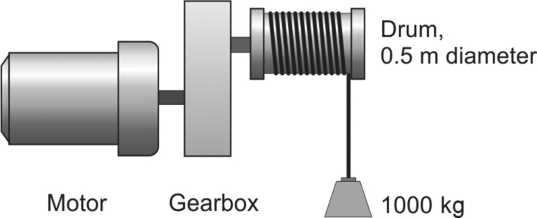
The drum diameter is 0.5 m, so if the maximum load (including the cable) is say 1000 kg, the tension in the cable (mg) will be 9810 N, and the torque applied by the load at the drum will be given by Force × radius = 9810 × 0.25 ≈ 2500 Nm. When the speed is constant (i.e. the load is not accelerating), the torque provided by the motor at the drum must be equal and opposite to that exerted at the drum by the load. (The word ‘opposite’ in the last sentence is often omitted, it being understood that steady-state motor and load torque must necessarily act in opposition.)
Suppose that the hoisting speed is to be controllable at any value up to a maximum of 0.5 m/s, and that we want this to correspond with a maximum motor speed of around 1500 rev/min, which is a reasonable speed for a wide range of motors. A hoisting speed of 0.5 m/s corresponds to a drum speed of 19 rev/min, so a suitable gear ratio would be say 80:1, giving a maximum motor speed of 1520 rev/min.
The load torque, as seen at the motor side of the gearbox, will be reduced by a factor of 80, from 2500 Nm to 31 Nm at the motor. We must also allow for friction in the gearbox, equivalent to perhaps 20% of the full load torque, so the maximum motor torque required for hoisting will be 37 Nm, and this torque must be available at all speeds up to the maximum of 1520 rev/min.
We can now draw the steady-state torque-speed curve of the load as seen by the motor, as shown in Fig. 11.8.
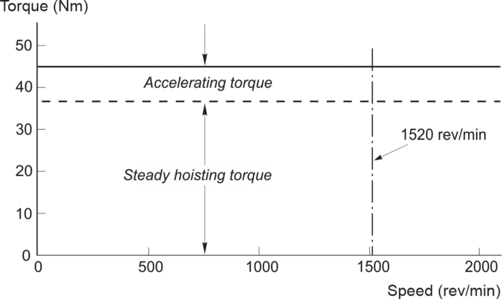
The steady-state motor power is obtained from the product of torque (Nm) and angular velocity (rad/s). The maximum continuous motor power for hoisting is therefore given by
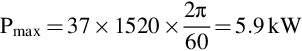
At this stage it is always a good idea to check that we would obtain roughly the same answer for the power by considering the work done per second at the load. The force (F) on the load is 9810 N, the velocity (v) is 0.5 m/s so the power (Fv) is 4.9 kW. This is 20% less than we obtained above, because here we have ignored the power lost in the gearbox.
So far we have established that we need a motor capable of continuously delivering 5.9 kW at 1520 rev/min in order to lift the heaviest load at the maximum required speed. However we have not yet addressed the question of how the load is accelerated from rest and brought up to the maximum speed. During the acceleration phase the motor must produce a torque greater than the load torque, or else the load will descend as soon as the brake is lifted. The greater the difference between the motor torque and the load torque, the higher the acceleration. Suppose we want the heaviest load to reach full speed from rest in say 1 s, and suppose we decide that the acceleration is to be constant. We can calculate the required accelerating torque from the equation of motion, i.e.

We usually find it best to work in terms of the variables as seen by the motor, and therefore we first need to find the effective total inertia as seen at the motor shaft, then calculate the motor acceleration, and finally use Eq. (11.2) to obtain the accelerating torque.
The effective inertia consists of the inertia of the motor itself, the referred inertia of the drum and gearbox, and the referred inertia of the load on the hook. The term ‘referred inertia’ means the apparent inertia, viewed from the motor side of the gearbox. If the gearbox has a ratio of n:1 (where n is greater than 1), an inertia of J on the low-speed side appears to be an inertia of J/n2 at the high-speed side. In this example the load actually moves in a straight line, so we need to ask what the effective inertia of the load is, as ‘seen’ at the drum. The geometry here is simple, and it is not difficult to see that as far as the inertia seen by the drum is concerned the load appears to be fixed to the surface of the drum. The load inertia at the drum is then obtained by using the formula for the inertia of a mass m located at radius r, i.e. J = mr2, yielding the effective load inertia at the drum as 1000 kg × (0.25 m)2 = 62.5 kgm2.
The effective inertia of the load as seen by the motor is 1/(80)2 × 62.5 ≈ 0.01 kgm2. To this must be added firstly the motor inertia which we can obtain by consulting the manufacturer’s catalogue for a 5.9 kW, 1520 rev/min motor. This will be straightforward for a d.c. motor, but a.c. motor catalogues tend to give ratings at utility frequencies only, and here a motor with the right torque needs to be selected, and the possible torque speed curve for the type of drive considered. For simplicity let us assume we have found a motor of precisely the required rating which has a rotor inertia of 0.02 kgm2. The referred inertia of the drum and gearbox, must be added and this again we have to calculate or look up. Suppose this yields a further 0.02 kgm2. The total effective inertia is thus 0.05 kgm2, of which 40% is due to the motor itself.
The acceleration is straightforward to obtain, since we know the motor speed is required to rise from zero to 1520 rev/min in 1 s. The angular acceleration is given by the increase in speed divided by the time taken, i.e.

We can now calculate the accelerating torque from Eq. (11.2) as
Hence in order to meet both the steady-state and dynamic torque requirements, a drive capable of delivering a torque of 45 Nm (= 37 + 8) at all speeds up to 1520 rev/min is required, as indicated in Fig. 11.8.
In the case of a hoist, the anticipated pattern of operation may not be known, but it is likely that the motor will spend most of its time hoisting rather than accelerating. Hence although the peak torque of 45 Nm must be available at all speeds, this will not be a continuous demand, and will probably be within the short-term overload capability of a drive which is continuously rated at 5.9 kW.
We should also consider what happens if it is necessary to lower the fully-loaded hook. We allowed for friction of 20% of the load torque (31 Nm), so during descent we can expect the friction to exert a braking torque equivalent to 6.2 Nm. But in order to prevent the hook from running-away, we will need a total torque of 31 Nm, so to restrain the load, the motor will have to produce a torque of 24.8 Nm. We would naturally refer to this as a braking torque because it is necessary to prevent the load on the hook from running away, but in fact the torque remains in the same direction as when hoisting. The speed is however negative, and in terms of a ‘four-quadrant’ diagram (e.g. Fig. 3.12) we have moved from quadrant 1 into quadrant 4, and thus the power flow is reversed and the motor is regenerating, the loss of potential energy of the descending load being converted back into electrical form (and losses). Hence if we wish to cater for this situation we must go for a drive that is capable of continuous regeneration: such a drive would also have the facility for operating in quadrant 3 to produce negative torque to drive down the empty hook if its weight was insufficient to lower itself.
In this example the torque is dominated by the steady-state requirement, and the inertia-dependent accelerating torque is comparatively modest. Of course if we had specified that the load was to be accelerated in one fifth of a second rather than 1 s, we would require an accelerating torque of 40 Nm rather than 8 Nm, and as far as torque requirements are concerned the acceleration torque would be more or less the same as the steady-state running torque. In this case it would be necessary to consult the drive manufacturer to determine the drive rating, which would depend on the frequency of the start/stop sequence.
The question of how to rate the motor when the loading is intermittent is explored more fully later, but it is worth noting that if the inertia is appreciable the stored rotational kinetic energy (![]() ) may become very significant, especially when the drive is required to bring the load to rest. Any stored energy either has to be dissipated in the motor and drive itself, or returned to the supply. All motors are inherently capable of regenerating, so the arrangement whereby the kinetic energy is recovered and dumped as heat in a resistor within the drive enclosure is the cheaper option, but is only practicable when the energy to be absorbed is modest. If the stored kinetic energy is large, the drive must be capable of returning energy to the supply, and this inevitably pushes up the cost of the converter.
) may become very significant, especially when the drive is required to bring the load to rest. Any stored energy either has to be dissipated in the motor and drive itself, or returned to the supply. All motors are inherently capable of regenerating, so the arrangement whereby the kinetic energy is recovered and dumped as heat in a resistor within the drive enclosure is the cheaper option, but is only practicable when the energy to be absorbed is modest. If the stored kinetic energy is large, the drive must be capable of returning energy to the supply, and this inevitably pushes up the cost of the converter.
In the case of our hoist, the stored kinetic energy is only

or about 1% of the energy needed to heat up a mug of water for a cup of coffee. Such modest energies could easily be absorbed by a resistor, but given that in this instance we are providing a regenerative drive, this energy would also be returned to the supply.
11.4.2 Inertia matching
There are some applications where the inertia dominates the torque requirement, and the question of selecting the right gearbox ratio has to be addressed. In this context the term ‘inertia matching’ often causes confusion, so it is worth explaining what it means.
Suppose we have a motor with a given torque, and we want to drive an inertial load via a gearbox. As discussed previously, the gear ratio determines the effective inertia as ‘seen’ by the motor: a high step-down ratio (i.e. load speed much less than motor speed) leads to a very low referred inertia, and vice-versa.
If the specification calls for the acceleration of the load to be maximised, it turns out that the optimum gear ratio is that which causes the referred inertia of the load to be equal to the inertia of the motor. Applications in which load acceleration is important include all types of positioning drives, e.g. in machine tools and phototypesetting. This explains why brushless PM synchronous motors, discussed in Chapter 9, are available from a wide range of manufacturers with different inertias. (There is an electrical parallel here—to get the most power into a load from a source with internal resistance R, the load resistance must be made equal to R.)
It is important to note however that inertia matching only maximises the acceleration of the load. Frequently it turns out that some other aspect of the specification (e.g. the maximum required load speed) cannot be met if the gearing is chosen to satisfy the inertia matching criterion, and it then becomes necessary to accept reduced acceleration of the load in favour of higher speed.
11.4.3 Fan and pump loads
Fans and centrifugal pumps have steady-state torque-speed characteristics which generally have the shape shown in Fig. 11.9.
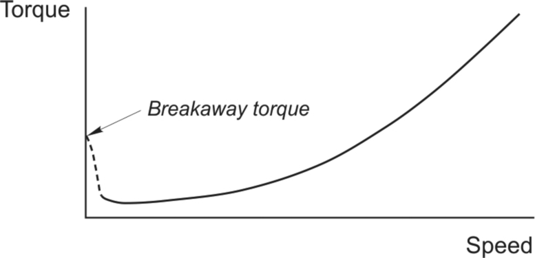
These characteristics are often approximately represented by assuming that the torque required is proportional to the square of the speed, and thus power proportional to the cube of the speed. We should note however that the approximation is seldom valid at low speeds because most real fans or pumps have a significant static friction or breakaway torque (as shown in Fig. 11.9) which must be overcome when starting.
When we consider the power-speed relationships the striking difference between the constant-torque and fan-type load is underlined. If the motor is rated for continuous operation at the full speed, it will be very lightly loaded (typically around 12% rated power) at half-speed, whereas with the constant torque load the power rating will be 50% at half speed. Fan-type loads which require speed control can therefore be handled by drives such as the inverter-fed cage induction motor, which can run happily at reduced speed and very much reduced torque without the need for additional cooling. If we assume that the rate of acceleration required is modest, the motor will require a torque-speed characteristic which is just a little greater than the load torque at all speeds. This defines the operating region in the torque-speed plane, from which the drive can be selected.
Many fans, which are required to operate almost continuously at rated speed, do not require speed control of course, and are well served by utility-frequency induction motors.
11.5 General application considerations
11.5.1 Regenerative operation and braking
All motors are inherently capable of regenerative operation, but in drives the basic power converter as used for the ‘bottom of the range’ version will not normally be capable of continuous regenerative operation. The cost of providing for fully regenerative operation is usually considerable, and users should always ask the question ‘do I really need it?’
In most cases it is not the recovery of energy for its own sake which is of prime concern, but rather the need to achieve a specified dynamic performance. Where rapid reversal is called for, for example, kinetic energy has to be removed quickly, and, as discussed in the previous section, this implies that the energy is either returned to the supply (regenerative operation) or dissipated (usually in a braking resistor). An important point to bear in mind is that a non-regenerative drive will have an asymmetrical transient speed response, so that when a higher speed is demanded, the extra kinetic energy can be provided quickly, but if a lower speed is demanded, the drive can do no better than reduce the torque to zero and allow the speed to coast down.
11.5.2 Duty cycle and rating
This is a complex matter, which in essence reflects the fact that whereas all motors are governed by a thermal (temperature rise) limitation, there are different patterns of operation which can lead to the same ultimate temperature rise.
Broadly speaking the procedure is to choose the motor on the basis of the root mean square of the power cycle, on the assumption that the losses (and therefore the temperature rise) vary with the square of the load. This is a reasonable approximation for most motors, especially if the variation in power is due to variations in load torque at an essentially constant speed, as is often the case, and the thermal time-constant of the motor is long compared with the period of the loading cycle. (The thermal time-constant has the same significance as it does in relation to any first-order linear system, e.g. an R/C circuit. If the motor is started from ambient temperature and run at a constant load, it takes typically four or five time-constants to reach its steady operating temperature.) Thermal time-constants vary from more than an hour for the largest motors (e.g. in a steel mill) through tens of minutes for medium power machines down to minutes for fractional-horsepower motors and seconds for small stepping motors.
To illustrate the estimation of rating when the load varies periodically, suppose a constant-frequency cage induction motor is required to run at a power of 4 kW for 2 min, followed by 2 min running light, then 2 min at 2 kW, then 2 min running light, this 8-min pattern being repeated continuously. To choose an appropriate power rating we need to find the r.m.s. power, which means exactly what it says, i.e. it is the square root of the mean (average) of the square of the power. The variation of power is shown in the upper part of Fig. 11.10, which has been drawn on the basis that when running light the power is negligible. The ‘power squared’ is shown in the lower part of the figure.

The average power is 1.5 kW, the average of the power squared is 5 kW2, and the r.m.s. power is therefore √ 5 kW, i.e. 2.24 kW. A motor that is continuously rated at 2.24 kW would therefore be suitable for this application, provided of course that it is capable of meeting the overload torque associated with the 4 kW period. The motor must therefore be able to deliver a torque that is greater than the continuous rated torque by a factor of 4/2.25, i.e. 178%: this would be within the capability of most general-purpose induction motors.
Motor suppliers are accustomed to recommending the best type of motor for a given pattern of operation, and they will typically classify the duty type in one of eight standard categories which cover the most commonly encountered modes of operation. As far as rating is concerned the most common classifications are maximum continuous rating, where the motor is capable of operating for an unlimited period, and short time rating, where the motor can only be operated for a limited time (typically 10, 30 or 60 min) starting from ambient temperature. NEMA, in the United States, refer to motor duty cycles in terms of continuous, intermittent or special duty. IEC 60034-1 defines duty cycles in eight ratings S1 … S8.
It is important to add that in controlled speed applications, the duty cycle also impacts the power electronic converter and here the thermal time constants are VERY much shorter than in the motor. The duty cycle can be very important in some applications, and should be clearly stated in a torque and speed-time profile to ensure that there is no ambiguity that could lead to subsequent disappointment.
11.5.3 Enclosures and cooling
There is clearly a world of difference between the harsh environment faced by a winch motor on the deck of an ocean-going ship and the comparative comfort enjoyed by a motor driving the drum of an office photocopier. The former must be protected against the ingress of rain and sea water, while the latter can rely on a dry and largely dust-free atmosphere.
Classifying the extremely diverse range of environments poses a potential problem, but fortunately this is one area where international standards have been agreed and are widely used. The International Electrotechnical Committee (IEC) standards for motor enclosures are now almost universal and take the form of a classification number prefixed by the letters IP, and followed by two digits. The first digit indicates the protection level against ingress of solid particles ranging from 1 (solid bodies greater than 50 mm diameter) to 5 (dust), while the second relates to the level of protection against ingress of water ranging from 1 (dripping water) through 5 (jets of water) to 8 (submersible). A zero in either the first or second digit indicates no protection.
Methods of motor cooling have also been classified and the more common arrangements are indicated by the letters IC followed by two digits, the first of which indicates the cooling arrangement (e.g. 4 indicates cooling through the surface of the frame of the motor) while the second shows how the cooling circuit power is provided (e.g. 1 indicates motor driven fan).
The most common motor enclosures for standard industrial electrical machines are IP 21 and 23 for d.c. motors; IP 44 and 54 for induction motors; and IP 65 and 66 for brushless PM synchronous motors. These classifications are known in the United States, but it is common practice for manufacturers there to adopt less formal designations, for example the following:
Open Drip Proof (ODP): Motors with ventilating openings, which permit passage of external cooling air over and around the windings. (Similar to IP23)
Totally Enclosed Fan Cooled (TEFC): A fan is attached to the shaft to push air over the frame during operation to enhance the cooling process. (Similar to IP54)
Washdown Duty (W): An enclosure designed for use in the food processing industry and other applications routinely exposed to washdown, chemicals, humidity and other severe environments. (Similar to IP65)
11.5.4 Dimensional standards
Standardisation is improving in this area, though it remains far from universal. Such matters as shaft diameter, centre height, mounting arrangements, terminal box position, and overall dimensions are fairly closely defined for the mainstream motors (induction, d.c.) over a wide size range, but standardisation is relatively poor at the low-power end because so many motors are tailor-made for specific applications.
Standardisation is also poor in relation to brushless PM motors. Paradoxically, the lack of standardisation, particularly in terms of frame size, mounting arrangements and shaft dimensions, has been cited as a significant driver of innovation in these machines, whereas the induction motor has been handicapped by its universal success and resulting standardisation!
11.5.5 Supply interaction and harmonics
As we have seen in Section 8.5, most converter-fed drives cause distortion of the utility voltage which can upset other sensitive equipment, particularly in the immediate vicinity of the installation. We have also discussed some of the options available to mitigate such effects. This is however a complex subject area and one which, in most cases, requires a systems overview rather than consideration of a single drive or even group of drives. It requires an intimate knowledge of the supply system, particularly its impedances.
With more and larger drives being installed, the problem of distortion is increasing, and supply authorities therefore react by imposing increasingly stringent statutory limits governing what is allowable.
The usual pattern is for the supply authority to specify the maximum amplitude and spectrum of the harmonic currents at the point of supply to a particular customer. If the proposed installation exceeds these limits, appropriate filter circuits must be connected in parallel with the installation. These can be costly, and their design is far from simple because the electrical characteristics of the supply system need to be known in advance in order to avoid unwanted resonance phenomena. Users need to be alert to the potential problem and, where appropriate, ensure that the drive supplier takes responsibility for handling it.
Measurement of harmonic currents is not straightforward and here the standards help, with IEC 61000-4-7:2002 providing valuable guidance.
11.6 Review questions
- (1) The speed-holding accuracy of a 1500 rev/min drive is specified as 0.5% at all speeds below base speed. If the speed reference is set at 75 rev/min, what are the maximum and minimum speeds between which the drive can claim to meet the specification?
- (2) A servo motor drives an inertial load via a toothed belt. The motor carries a 12-tooth pulley, and the total inertia of motor and pulley is 0.001 kgm2. The load inertia (including the load pulley) is 0.009 kgm2. Find the number of teeth on the load pulley that will maximise the acceleration of the load.
- (3) Assuming that the temperature rise of a motor follows an exponential curve, that the final temperature rise is proportional to the total losses and that the losses are proportional to the square of the load power, for how long could a motor with a 30-min thermal time-constant be started from cold and overloaded by 60%?
- (4) A special-purpose numerically-controlled machine-tool spindle has a maximum speed of 10,000 rev/min, and requires full torque at all speeds. Peak steady-state power is of the order of 1200 W. The manufacturer wishes to use a direct-drive motor. Discuss options, and suggest what additional information might be required in order to seek the best solution.
- (5) When planning to purchase a variable-frequency inverter to provide speed control of an erstwhile fixed-frequency induction motor driving a hoist, what problems should be anticipated if low-speed operation is envisaged?
- (6) List two controlled-speed applications for which conventional d.c. motors are not suitable, and suggest an alternative for each.
- (7) A standard induction motor can produce twice full load for short periods, but a standard inverter is limited to its rated output. What accounts for the difference?
- (8) A pump drive supplied from the 50 Hz utility supply requires a torque of 60 Nm at approximately 1400 rev/min for 1 min, followed by 5 min during which the motor runs unloaded. This cyclic pattern is repeated continuously.
The motor is to be selected from a range of general-purpose cage motors with continuous ratings of 2.2, 3, 4, 5.5, 7.5, 11 and 15 kW. The motors all have full-load slips of approximately 5% and pull-out torques of 200% at slips of approximately 15%.
Select the pole number and power rating, and estimate the running speed when the motor drives the pump. - (9) A speed-controlled drive rated 50 kW at its base speed of 1200 rev/min drives a large circular stone-cutting saw. When the drive is started from rest with the speed reference set to base speed, it accelerates to 1180 rev/min in 4 s, during which time the acceleration is more-or-less uniform. It takes a further second to settle at full speed, after which time the saw engages with the workpiece.
Estimate the total effective inertia of motor and saw. Make clear what assumptions you have had to make. Estimate the stored kinetic energy at full speed, and compare it with the energy supplied during the first 4 s. - (10) When the saw in question 9 is running light at base speed, and the power is switched-off, the speed falls approximately linearly, taking 20 s to reach 90% of base speed. Estimate the friction torque as a percentage of the full-load torque of the motor. Explain how this result justifies any approximations that had to be made in order to answer question 9.
Answers to review questions are given in the Appendix.