Electric motors—The basics
Abstract
Non-specialist readers wishing to learn the essence of how and why motors work will find answers in this chapter. We discuss how to quantify magnetic effects, explain how force and torque are generated, and show that the elegant energy-converting process can be predicted using a simple equivalent circuit. The key factors that underpin the operation of all types of motor emerge, and we conclude by identifying the simple design parameters that determine the relationship between rotor volume and torque.
Keywords
Magnetic field; Magnetomotive force (m.m.f.); Magnetic circuit; Reluctance; Torque; Motional e.m.f.; Energy conversion; Primitive motor
1.1 Introduction
Electric motors are so much a part of everyday life that we seldom give them a second thought. When we switch on an ancient electric drill, for example, we confidently expect it to run rapidly up to the correct speed, and we don’t question how it knows what speed to run at, nor how it is that once enough energy has been drawn from the supply to bring it up to speed, the power drawn falls to a very low level. When we put the drill to work it draws more power, and when we finish the power drawn from the supply reduces automatically, without intervention on our part.
The humble motor, consisting of nothing more than an arrangement of copper coils and steel laminations, is clearly rather a clever energy converter, which warrants serious consideration. By gaining a basic understanding of how the motor works, we will be able to appreciate its potential and its limitations, and (in later chapters) see how its already remarkable performance is dramatically enhanced by the addition of external electronic controls.
The great majority of electric motors have a shaft which rotates, but linear electric motors have niche applications, and whilst they appear very different from their rotating sister, their principle of operation is the same.
This chapter deals with the basic mechanisms of motor operation, so readers who are already familiar with such matters as magnetic flux, magnetic and electric circuits, torque, and motional e.m.f. (electromotive force) can probably afford to skim over much of it. In the course of the discussion, however, several very important general principles and guidelines emerge. These apply to all types of motor and are summarised in Section 1.9. Experience shows that anyone who has a good grasp of these basic principles will be well equipped to weigh the pros and cons of the different types of motor, so all readers are urged to absorb them before tackling other parts of the book.
1.2 Producing rotation
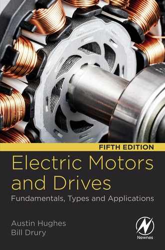
Nearly all motors exploit the force which is exerted on a current-carrying conductor placed in a magnetic field. The force can be demonstrated by placing a bar magnet near a wire carrying current (Fig. 1.1), but anyone trying the experiment will probably be disappointed to discover how feeble the force is, and will doubtless be left wondering how such an unpromising effect can be used to make effective motors.
We will see that in order to make the most of the mechanism, we need to arrange for there to be a very strong magnetic field, and for it to interact with many conductors, each carrying as much current as possible. We will also see later that although the magnetic field (or ‘excitation’) is essential to the working of the motor, it acts only as a catalyst, and all of the mechanical output power comes from the electrical supply to the conductors on which the force is developed.
It will emerge later that in some motors the parts of the machine responsible for the excitation and for the energy converting functions are distinct and self-evident. In the d.c. motor, for example, the excitation is provided either by permanent magnets or by field coils wrapped around clearly-defined projecting field poles on the stationary part, while the conductors on which force is developed are on the rotor and supplied with current via sliding contacts known as brushes. In many motors, however, there is no such clear-cut physical distinction between the ‘excitation’ and the ‘energy-converting’ parts of the machine, and a single stationary winding serves both purposes. Nevertheless, we will find that identifying and separating the excitation and energy-converting functions is always helpful to understanding both how motors of all types operate, and their performance characteristics.
Returning to the matter of force on a single conductor, we will look first at what determines the magnitude and direction of the force, before turning to ways in which the mechanism is exploited to produce rotation. The concept of the magnetic circuit will have to be explored, since this is central to understanding why motors have the shapes they do. Before that a brief introduction to the magnetic field and magnetic flux and flux density is included for those who are not already familiar with the ideas involved.
1.2.1 Magnetic field and magnetic flux
When a current-carrying conductor is placed in a magnetic field, it experiences a force. Experiment shows that the magnitude of the force depends directly on the current in the wire, and the strength of the magnetic field, and that the force is greatest when the magnetic field is perpendicular to the conductor.
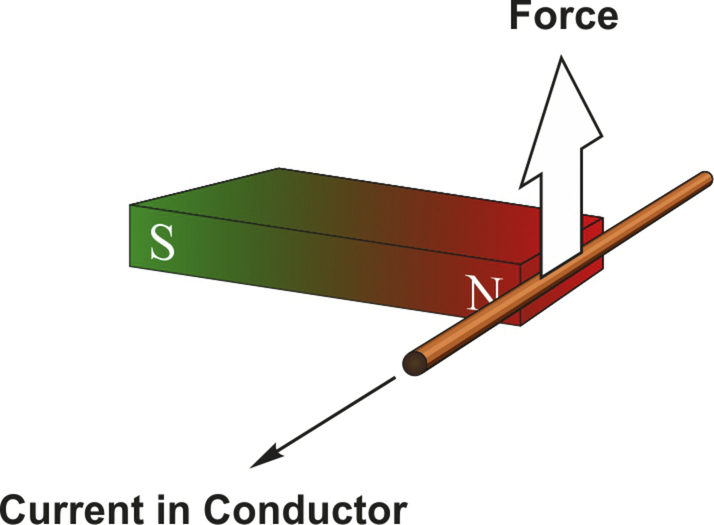
In the set-up shown in Fig. 1.1, the source of the magnetic field is a bar magnet, which produces a magnetic field as shown in Fig. 1.2.
The notion of a ‘magnetic field’ surrounding a magnet is an abstract idea that helps us to come to grips with the mysterious phenomenon of magnetism: it not only provides us with a convenient pictorial way of picturing the directional effects, but it also allows us to quantify the ‘strength’ of the magnetism and hence permits us to predict the various effects produced by it.
The dotted lines in Fig. 1.2 are referred to as magnetic flux lines, or simply flux lines. They indicate the direction along which iron filings (or small steel pins) would align themselves when placed in the field of the bar magnet. Steel pins have no initial magnetic field of their own, so there is no reason why one end or the other of the pins should point to a particular pole of the bar magnet.
However, when we put a compass needle (which is itself a permanent magnet) in the field we find that it aligns itself as shown in Fig. 1.2. In the upper half of the figure, the S end of the diamond-shaped compass settles closest to the N pole of the magnet, while in the lower half of the figure, the N end of the compass seeks the S of the magnet. This immediately suggests that there is a direction associated with the lines of flux, as shown by the arrows on the flux lines, which conventionally are taken as positively directed from the N to the S pole of the bar magnet.
The sketch in Fig. 1.2 might suggest that there is a ‘source’ near the top of the bar magnet, from which flux lines emanate before making their way to a corresponding ‘sink’ at the bottom. However, if we were to look at the flux lines inside the magnet, we would find that they were continuous, with no ‘start’ or ‘finish’. (In Fig. 1.2 the internal flux lines have been omitted for the sake of clarity, but a very similar field pattern is produced by a circular coil of wire carrying a direct current—see Fig. 1.7 where the continuity of the flux lines is clear.) Magnetic flux lines always form closed paths, as we will see when we look at the ‘magnetic circuit’, and draw a parallel with the electric circuit, in which the current is also a continuous quantity. (There must be a ‘cause’ of the magnetic flux, of course, and in a permanent magnet this is usually pictured in terms of atomic-level circulating currents within the magnet material. Fortunately, discussion at this physical level is not necessary for our purposes.)
1.2.2 Magnetic flux density
As well as showing direction, the flux plots also convey information about the intensity of the magnetic field. To achieve this, we introduce the idea that between every pair of flux lines (and for a given depth into the paper) there is the same ‘quantity’ of magnetic flux. Some people have no difficulty with such a concept, while others find that the notion of quantifying something so abstract represents a serious intellectual challenge. But whether the approach seems obvious or not, there is no denying the practical utility of quantifying the mysterious stuff we call magnetic flux, and it leads us next to the very important idea of magnetic flux density (B).
When the flux lines are close together, the ‘tube’ of flux is squashed into a smaller space, whereas when the lines are further apart the same tube of flux has more breathing space. The flux density (B) is simply the flux in the ‘tube’ (Φ) divided by the cross-sectional area (A) of the tube, i.e.
The flux density is a vector quantity, and is therefore often written in bold type: its magnitude is given by Eq. (1.1), and its direction is that of the prevailing flux lines at each point. Near the top of the magnet in Fig. 1.2, for example, the flux density will be large (because the flux is squashed into a small area), and pointing upwards, whereas on the equator and far out from the body of the magnet the flux density will be small and directed downwards.
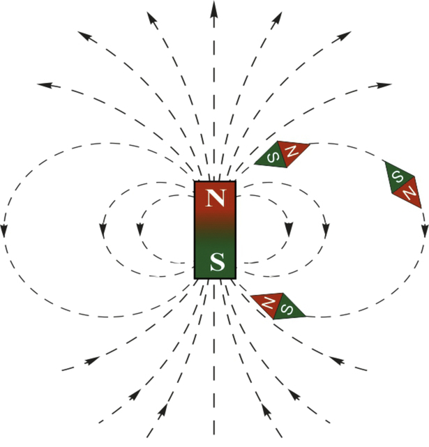
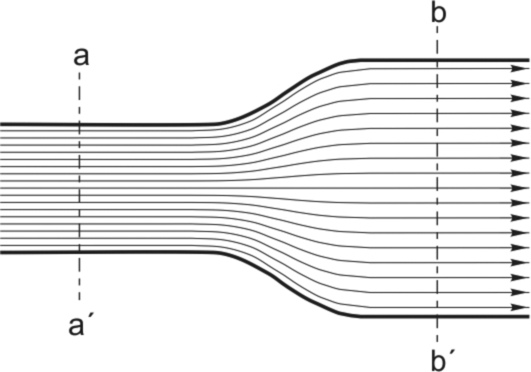
We will see later that in order to create high flux densities in motors, the flux spends most of its life inside well-defined ‘magnetic circuits’ made of iron or steel, within which the flux lines spread out uniformly to take full advantage of the available area. In the case shown in Fig. 1.3, for example, the cross-sectional area of the iron at bb’ is twice that at aa’, but the flux is constant so the flux density at bb’ is half that at aa’.
It remains to specify units for quantity of flux, and flux density. In the SI system, the unit of magnetic flux is the Weber (Wb). If one Weber of flux is distributed uniformly across an area of one square metre perpendicular to the flux, the flux density is clearly one Weber per square metre (Wb/m2). This was the unit of B until about 60 years ago, when it was decided that one Weber per square metre would henceforth be known as one Tesla (T), in honour of Nikola Tesla whose is generally credited with inventing the induction motor. The widespread use of B (measured in Tesla) in the design stage of all types of electromagnetic apparatus means that we are constantly reminded of the importance of Tesla; but at the same time one has to acknowledge that the outdated unit did have the advantage of conveying directly what flux density is, i.e. flux divided by area.
The flux in a 1 kW motor will be perhaps a few tens of milliwebers, and a small bar magnet would probably only produce a few microwebers. On the other hand, values of flux density are typically around 1 Tesla in most motors (regardless of type and rating), which is a reflection of the fact that although the quantity of flux in the 1 kW motor is small, it is also spread over a small area.
1.2.3 Force on a conductor
We now return to the production of force on a current-carrying wire placed in a magnetic field, as revealed by the set-up shown in Fig. 1.1.
The force is shown in Fig. 1.1: it is at right angles to both the current and the magnetic flux density, and its direction can be found using Fleming’s left hand rule. If we picture the thumb, first and middle fingers held mutually perpendicular, then the first finger represents the field or flux density (B), the middle finger represents the current (I), and the thumb then indicates the direction of motion, as shown in Fig. 1.4.

Clearly, if either the field or the current is reversed, the force acts downwards, and if both are reversed, the direction of the force remains the same.
We find by experiment that if we double either the current or the flux density, we double the force, while doubling both causes the force to increase by a factor of four. But how about quantifying the force? We need to express the force in terms of the product of the current and the magnetic flux density, and this turns out to be very straightforward when we work in SI units.
The force F on a wire of length l, carrying a current I and exposed to a uniform magnetic flux density B throughout its length is given by the simple expression
In Eq. (1.2), F is in Newtons when B is in Tesla, I in Amps, and l in metres.
This is a delightfully simple formula, and it may come as a surprise to some readers that there are no constants of proportionality involved in Eq. (1.2). The simplicity is not a coincidence, but stems from the fact that the unit of current (the Ampere) is actually defined in terms of force.
Eq. (1.2) only applies when the current is perpendicular to the field. If this condition is not met, the force on the conductor will be less; and in the extreme case where the current was in the same direction as the field, the force would fall to zero. However, every sensible motor designer knows that to get the best out of the magnetic field it has to be perpendicular to the conductors, and so it is safe to assume in the subsequent discussion that B and I are always perpendicular. In the remainder of this book, it will be assumed that the flux density and current are mutually perpendicular, and this is why, although B is a vector quantity (and would usually be denoted by bold type), we can drop the bold notation because the direction is implicit and we are only interested in the magnitude.
The reason for the very low force detected in the experiment with the bar magnet is revealed by Eq. (1.2). To obtain a high force, we must have a high flux density, and a lot of current. The flux density at the ends of a bar magnet is low, perhaps 0.1 Tesla, so a wire carrying 1 Amp will experience a force of only 0.1 N (approximately 10 g wt) per metre. Since the flux density will be confined to perhaps 1 cm across the end face of the magnet, the total force on the wire will be only 0.1 g wt. This would be barely detectable, and is too low to be of any use in a decent motor. So how is more force obtained?
The first step is to obtain the highest possible flux density. This is achieved by designing a ‘good’ magnetic circuit, and is discussed next. Secondly, as many conductors as possible must be packed in the space where the magnetic field exists, and each conductor must carry as much current as it can without heating up to a dangerous temperature. In this way, impressive forces can be obtained from modestly sized devices, as anyone who has tried to stop an electric drill by grasping the chuck will testify.
1.3 Magnetic circuits
So far we have assumed that the source of the magnetic field is a permanent magnet. This is a convenient starting point as all of us are familiar with magnets. But in the majority of motors, the magnetic field is produced by coils of wire carrying current, so it is appropriate that we look at how we arrange the coils and their associated ‘magnetic circuit’ so as to produce high magnetic fields which then interact with other current-carrying conductors to produce force, and hence rotation.
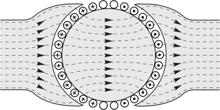
First, we look at the simplest possible case of the magnetic field surrounding an isolated long straight wire carrying a steady current (Fig. 1.5). (In the figure, the + sign indicates that current is flowing into the paper, while a dot is used to signify current out of the paper: these symbols can perhaps be remembered by picturing an arrow or dart, with the cross being the rear view of the fletch, and the dot being the approaching point.) The flux lines form circles concentric with the wire, the field strength being greatest close to the wire. As might be expected, the field strength at any point is directly proportional to the current. The convention for determining the direction of the field is that the positive direction is taken to be the direction that a right-handed corkscrew must be rotated to move in the direction of the current.
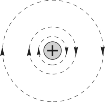
Fig. 1.5 is somewhat artificial as current can only flow in a complete circuit, so there must always be a return path. If we imagine a parallel ‘go’ and ‘return’ circuit, for example, the field can be obtained by superimposing the field produced by the positive current in the go side with the field produced by the negative current in the return side, as shown in Fig. 1.6.
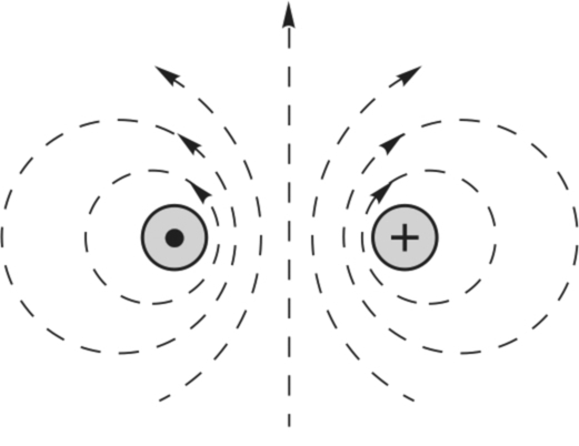

We note how the field is increased in the region between the conductors, and reduced in the regions outside. Although Fig. 1.6 strictly only applies to an infinitely long pair of straight conductors, it will probably not come as a surprise to learn that the field produced by a single turn of wire of rectangular, square or round form is very much the same as that shown in Fig. 1.6. This enables us to build up a picture of the field that would be produced—in air—by the sort of coils used in motors, which typically have many turns, as shown for example in Fig. 1.7.
The coil itself is shown on the left in Fig. 1.7 while the flux pattern produced is shown on the right. Each turn in the coil produces a field pattern, and when all the individual field components are superimposed we see that the field inside the coil is substantially increased and that the closed flux paths closely resemble those of the bar magnet that we looked at earlier. The air surrounding the sources of the field offers a homogeneous path for the flux, so once the tubes of flux escape from the concentrating influence of the source, they are free to spread out into the whole of the surrounding space. Recalling that between each pair of flux lines there is an equal amount of flux, we see that because the flux lines spread out as they leave the confines of the coil, the flux density is much lower outside than inside: for example, if the distance ‘b’ is say four times ‘a’ the flux density Bb is a quarter of Ba.
Although the flux density inside the coil is higher than outside, we would find that the flux densities which we could achieve are still too low to be of use in a motor. What is needed is firstly a way of increasing the flux density, and secondly a means for concentrating the flux and preventing it from spreading out into the surrounding space.
1.3.1 Magnetomotive force (m.m.f.)
One obvious way to increase the flux density is to increase the current in the coil, or to add more turns. We find that if we double the current, or the number of turns, we double the total flux, thereby doubling the flux density everywhere.
We quantify the ability of the coil to produce flux in terms of its Magnetomotive Force (m.m.f.). The m.m.f. of the coil is simply the product of the number of turns (N) and the current (I), and is thus expressed in Ampere-turns. A given m.m.f. can be obtained with a large number of turns of thin wire carrying a low current, or a few turns of thick wire carrying a high current: as long as the product NI is constant, the m.m.f. is the same.
1.3.2 Electric circuit analogy
We have seen that the magnetic flux which is set up is proportional to the m.m.f. driving it. This points to a parallel with the electric circuit, where the current (Amps) which flows is proportional to the electromotive force (e.m.f., in Volts) driving it.
In the electric circuit, current and e.m.f. are related by Ohm’s Law, which is

For a given source e.m.f. (Volts), the current depends inversely on the resistance of the circuit, so to obtain more current, the resistance of the circuit has to be reduced.
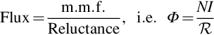
We can make use of an equivalent ‘magnetic Ohm’s law’ by introducing the idea of Reluctance (![]() ). The reluctance gives a measure of how difficult it is for the magnetic flux to complete its circuit, in the same way that resistance indicates how much opposition the current encounters in the electric circuit.
). The reluctance gives a measure of how difficult it is for the magnetic flux to complete its circuit, in the same way that resistance indicates how much opposition the current encounters in the electric circuit.
The magnetic Ohm’s law is then
We see from Eq. (1.4) that to increase the flux for a given m.m.f. we need to reduce the reluctance of the magnetic circuit. In the case of the example (Fig. 1.7), this means we must replace as much as possible of the air path (which is a ‘poor’ magnetic material, and therefore constitutes a high reluctance) with a ‘good’ magnetic material, thereby reducing the reluctance and resulting in a higher flux for a given m.m.f.
The material which we usually choose is good quality magnetic steel, which for historical reasons is often referred to as ‘iron’. This brings several very dramatic and desirable benefits, as shown in Fig. 1.8.

Firstly, the reluctance of the iron paths is very much less than the air paths which they have replaced, so the total flux produced for a given m.m.f. is very much greater. (Strictly speaking therefore, if the m.m.f.’s and cross-sections of the coils in Figs. 1.7 and 1.8 are the same, many more flux lines should be shown in Fig. 1.8 than in Fig. 1.7, but for the sake of clarity a similar number are indicated.) Secondly, almost all the flux is confined within the iron, rather than spreading out into the surrounding air. We can therefore shape the iron parts of the magnetic circuit as shown in Fig. 1.8 in order to guide the flux to wherever it is needed. And finally, we see that inside the iron, the flux density remains constant over the whole uniform cross-section, there being so little reluctance that there is no noticeable tendency for the flux to crowd to one side or another.
Before moving on to the matter of the air-gap, a question which is often asked is whether it is important for the coils to be wound tightly onto the magnetic circuit, and whether, if there is a multi-layer winding, the outer turns are as effective as the inner ones. The answer, happily, is that the total m.m.f. is determined solely by the number of turns and the current, and therefore every complete turn makes the same contribution to the total m.m.f., regardless of whether it happens to be tightly or loosely wound. Of course it does make sense for the coils to be wound as tightly as is practicable, since this not only minimises the resistance of the coil (and thereby reduces the heat loss) but also makes it easier for the heat generated to be conducted away to the frame of the machine.
1.3.3 The air-gap
In motors, we intend to use the high flux density to develop force on current-carrying conductors, which must then move to produce useful work. We have now seen how to create a high flux density in a magnetic circuit, but, of course, it is not possible to put current-carrying conductors inside the iron. We therefore arrange for an air-gap in the magnetic circuit, as shown in Fig. 1.8. We will see shortly (see for example Fig. 1.12) that the conductors on which the force is to be produced will be placed in this air-gap region. So although we will find that the reluctance of the air-gap is unwelcome from the magnetic circuit viewpoint, it is obviously necessary for there to be mechanical clearance to allow the rotor to rotate.
If the air-gap is relatively small, as in motors, we find that the flux jumps across the air-gap as shown in Fig. 1.8, with very little tendency to balloon out into the surrounding air. With most of the flux lines going straight across the air-gap, the flux density in the gap region has the same high value as it does inside the iron.
In the majority of magnetic circuits with one or more air-gaps, the reluctance of the iron parts is very much less than the reluctance of the gaps. At first sight this can seem surprising, since the distance across the gap is so much less than the rest of the path through the iron. The fact that the air-gap dominates the reluctance is simply a reflection of how poor air is as a magnetic medium, compared with iron. To put the comparison in perspective, if we calculate the reluctances of two paths of equal length and cross-sectional area, one being in iron and the other in air, the reluctance of the air path will typically be 1000 times greater than the reluctance of the iron path.
Returning to the analogy with the electric circuit, the role of the iron parts of the magnetic circuit can be likened to that of the copper wires in the electric circuit. Both offer little opposition to flow (so that a negligible fraction of the driving force (m.m.f. or e.m.f.) is wasted in conveying the flow to where it is usefully exploited) and both can be shaped to guide the flow to its destination. There is one important difference, however. In the electric circuit, no current will flow until the circuit is completed, after which all the current is confined inside the wires. With an iron magnetic circuit, some flux can flow (in the surrounding air) even before the iron is installed. And although most of the flux will subsequently take the easy route through the iron, some will still leak into the air, as shown in Fig. 1.8. We will not pursue leakage flux here, though it is sometimes important, as will be seen later.
1.3.4 Reluctance and air-gap flux densities
If we neglect the reluctance of the iron parts of a magnetic circuit, it is easy to estimate the flux density in the air-gap. Since the iron parts are then in effect ‘perfect conductors’ of flux, none of the source m.m.f. (NI) is used in driving the flux through the iron parts, and all of it is available to push the flux across the air-gap. The situation depicted in Fig. 1.8 therefore reduces to that shown in Fig. 1.9, where an m.m.f. of NI is applied directly across an air-gap of length g.
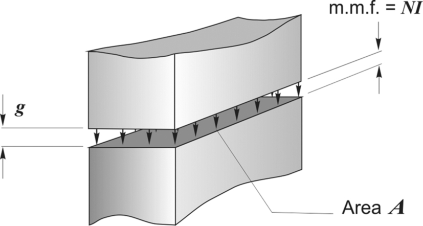
To determine how much flux will cross the gap, we need to know its reluctance. As might be expected the reluctance of any part of the magnetic circuit depends on its dimensions, and on its magnetic properties, and the reluctance of a rectangular ‘prism’ of air, of cross-sectional area A and length g is given by

where μ0 is the so-called ‘primary magnetic constant’ or ‘permeability of free space’. Strictly, as its name implies, μo quantifies the magnetic properties of a vacuum, but for all engineering purposes the permeability of air is also μo. The value of the primary magnetic constant (μo) in the SI system is 4π × 10− 7 Henry/m: rather surprisingly, there is no widely-used name for the unit of reluctance.
(In passing, we should note that if we want to include the reluctance of the iron part of the magnetic circuit in our calculation, its reluctance would be given by

and we would have to add this to the reluctance of the air-gap to obtain the total reluctance. However, as stated earlier, because the permeability of iron (μiron) is so much higher than μ0, its reluctance will be very much less than the gap reluctance, despite the path length liron being considerably longer than the path length (g) in the air.)
Eq. (1.5) reveals the expected result that doubling the air-gap would double the reluctance (because the flux has twice as far to go), while doubling the area would halve the reluctance (because the flux has two equally appealing paths in parallel). To calculate the flux, Φ, we use the magnetic Ohm’s law (Eq. 1.4), which gives

We are usually interested in the flux density in the gap, rather than the total flux, so we use Eq. (1.1) to yield
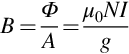
Eq. (1.7) is delightfully simple, and from it we can calculate the air-gap flux density once we know the m.m.f. of the coil (NI) and the length of the gap (g). We do not need to know the details of the coil-winding as long as we know the product of the turns and the current, and neither do we need to know the cross-sectional area of the magnetic circuit in order to obtain the flux density (though we do if we want to know the total flux, see Eq. 1.6).
For example, suppose the magnetising coil has 250 turns, the current is 2 A, and the gap is 1 mm. The flux density is then given by
(We could of course create the same flux density with a coil of 50 turns carrying a current of 10 A, or any other combination of turns and current giving an m.m.f. of 500 Ampere-turns.)
If the cross-sectional area of the iron was constant at all points, the flux density would be 0.63 T everywhere. Sometimes, as has already been mentioned, the cross-section of the iron reduces at points away from the air-gap, as shown for example in Fig. 1.3. Because the flux is compressed in the narrower sections, the flux density is higher, and in Fig. 1.3 if the flux density at the air-gap and in the adjacent pole-faces is once again taken to be 0.63 T, then at the section aa’ (where the area is only half that at the air-gap) the flux density will be 2 × 0.63 = 1.26 T.
1.3.5 Saturation
It would be reasonable to ask whether there is any limit to the flux density at which the iron can be operated. We can anticipate that there must be a limit, or else it would be possible to squash the flux into a vanishingly small cross-section, which we know is not the case. In fact there is a limit, though not a very sharply defined one.
Earlier we noted that the ‘iron’ has very little reluctance, at least not in comparison with air. Unfortunately this happy state of affairs is only true as long as the flux density remains below about 1.6–1.8 T, depending on the particular magnetic steel in question: if we try to work at higher flux densities, it begins to exhibit significant reluctance, and no longer behaves like an ideal conductor of flux. At these higher flux densities a significant proportion of the source m.m.f. is used in driving the flux through the iron. This situation is obviously undesirable, since less m.m.f. remains to drive the flux across the air-gap. So, just as we would not recommend the use of high-resistance supply leads to the load in an electric circuit, we must avoid overloading the iron parts of the magnetic circuit.
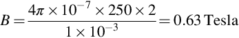
The emergence of significant reluctance as the flux density is raised is illustrated qualitatively in Fig. 1.10. When the reluctance begins to be appreciable, the iron is said to be beginning to ‘saturate’. The term is apt, because if we continue increasing the m.m.f. or reducing the area of the iron, we will eventually reach an almost constant flux density, typically around 2 T. To avoid the undesirable effects of saturation, the size of the iron parts of the magnetic circuit are usually chosen so that the flux density does not exceed about 1.5 T. At this level of flux density, the reluctance of the iron parts will remain small in comparison with the air-gap.
1.3.6 Magnetic circuits in motors
The reader may be wondering why so much attention has been focused on the gapped C-core magnetic circuit, when it appears to bear little resemblance to the magnetic circuits found in motors. We will now see that it is actually a short step from the C-core to a typical motor magnetic circuit, and that no fundamentally new ideas are involved.
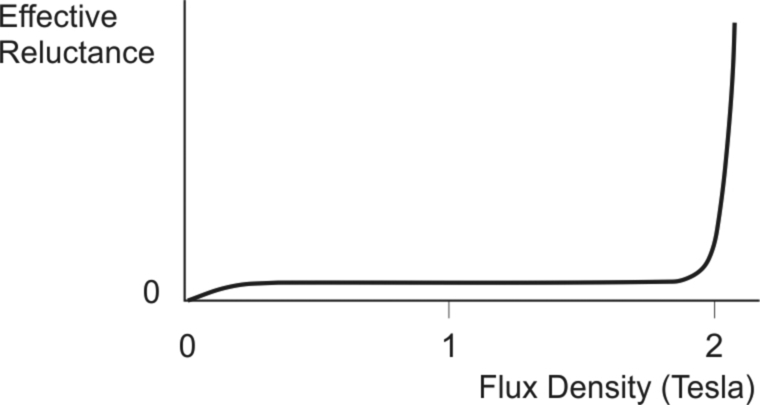
The evolution from C-core to motor geometry is shown in Fig. 1.11, which should be largely self-explanatory, and relates to the field system of a traditional d.c. motor.
We note that the first stage of evolution (Fig. 1.11, left) results in the original single gap of length g being split into two gaps of length g/2, reflecting the requirement for the rotor to be able to turn. At the same time the single magnetising coil is split into two to preserve symmetry. (Relocating the magnetising coil at a different position around the magnetic circuit is of course in order, just as a battery can be placed anywhere in an electric circuit.) Next, (Fig. 1.11, centre) the single magnetic path is split into two parallel paths of half the original cross-section, each of which carries half of the flux: and finally (Fig. 1.11, right), the flux paths and pole faces are curved to match the cylindrical rotor. The coil now has several layers in order to fit the available space, but as discussed earlier this has no adverse effect on the m.m.f. The air-gap is still small, so the flux crosses radially to the rotor.
1.4 Torque production
Having designed the magnetic circuit to give a high flux density under the poles, we must obtain maximum benefit from it. We therefore need to arrange a set of conductors, fixed to the rotor, as shown in Fig. 1.12, and to ensure that conductors under a N-pole (on the left) carry positive current (into the paper), while those under the S-pole carry negative current. The tangential electromagnetic (‘BIl’) force (see Eq. 1.2) on all the positive conductors will be downwards (towards the bottom of the page), while the force on the negative ones will be upwards (towards the top of the page): a torque will therefore be exerted on the rotor, which will be caused to rotate.
(The observant reader spotting that some of the conductors appear to have no current in them will find the explanation later, in Chapter 3.)
At this point we should pause and address three questions that often crop up when these ideas are being developed. The first is to ask why we have made no reference to the magnetic field produced by the current-carrying conductors on the rotor. Surely they too will produce a magnetic field, which will presumably interfere with the original field in the air-gap, in which case perhaps the expression used to calculate the force on the conductor will no longer be valid.
The answer to this very perceptive question is that the field produced by the current-carrying conductors on the rotor certainly will modify the original field (i.e. the field that was present when there was no current in the rotor conductors.) But in the majority of motors, the force on the conductor can be calculated correctly from the product of the current and the ‘original’ field. This is very fortunate from the point of view of calculating the force, but also has a logical feel to it. For example in Fig. 1.1, we would not expect any force on the current-carrying conductor if there was no externally applied field, even though the current in the conductor will produce its own field (upwards on one side of the conductor and downwards on the other). So it seems right that since we only obtain a force when there is an external field, all of the force must be due to that field alone. (In Chapter 3 we will discover that the field produced by the rotor conductors is known as ‘armature reaction’, and that, especially when the magnetic circuit becomes saturated, its undesirable effects may be combatted by fitting additional windings designed to nullify the armature field.)
The second question arises when we think about the action and reaction principle. When there is a torque on the rotor, there is presumably an equal and opposite torque on the stator; and therefore we might wonder if the mechanism of torque production could be pictured using the same ideas as we used for obtaining the rotor torque. The answer is yes, there is always an equal and opposite torque on the stator, which is why it is usually important to bolt a motor down securely. In some machines (e.g. the induction motor) it is easy to see that torque is produced on the stator by the interaction of the air-gap flux density and the stator currents, in exactly the same way that the flux density interacts with the rotor currents to produce torque on the rotor. In other motors (e.g. the d.c. motor we have been looking at), there is no simple physical argument which can be advanced to derive the torque on the stator, but nevertheless it is equal and opposite to the torque on the rotor.
The final question relates to the similarity between the set-up shown in Fig. 1.11 and the field patterns produced for example by the electromagnets used to lift car bodies in a scrap yard. From what we know of the large force of attraction that lifting magnets can produce, might we not expect there to be a large radial force between the stator pole and the iron body of the rotor? And if there is, what is to prevent the rotor from being pulled across to the stator?
Again the affirmative answer is that there is indeed a radial force due to magnetic attraction, exactly as in a lifting magnet or relay, although the mechanism whereby the magnetic field exerts a pull as it enters iron or steel is different from the ‘BIl ‘force we have been looking at so far.
It turns out that the force of attraction per unit area of pole-face is proportional to the square of the radial flux density, and with typical air-gap flux densities of up to 1 T in motors, the force per unit area of rotor surface works out to be about 40 N/cm2. This indicates that the total radial force can be very large: for example the force of attraction on a small pole face of only 5 cm × 10 cm is 2000 N, or about 200 kg. This force contributes nothing to the torque of the motor, and is merely an unwelcome by-product of the ‘BIl’ mechanism we employ to produce tangential force on the rotor conductors.
In most machines the radial magnetic force under each pole is actually a good deal bigger than the tangential electromagnetic force on the rotor conductors, and as the question implies, it tends to pull the rotor onto the pole. However, the majority of motors are constructed with an even number of poles equally spaced around the rotor, and the flux density in each pole is the same, so that—in theory at least—the resultant force on the complete rotor is zero. In practice, even a small eccentricity will cause the field to be stronger under the poles where the air-gap is smaller, and this will give rise to an unbalanced pull, resulting in noisy running and rapid bearing wear.
In the majority of motors we can quantify the torque via the ‘BIl’ approach. The source of the magnetic flux density B may be a winding, as in Fig. 1.11, or a permanent magnet. The source (or ‘excitation’) may be located on the stator (as implied in Fig. 1.12) or on the rotor. If the source of B is on the stator, the current carrying conductors on which the force is developed are located on the rotor, whereas if the excitation is on the rotor, the active conductors are on the stator. In all of these the large radial magnetic forces discussed above are an unwanted by-product.
However, in some motors the stator and/or rotor geometry is arranged so that some of the flux crossing the air-gap to the rotor produces tangential forces (and thus torque) directly on the rotor iron, without any rotor currents. We will see in later chapters that in some of these ‘reluctance’ machines, we can still quantify the torque using the ‘BIl’ method, while in others we have to employ an alternative to the ‘BIl’ method to obtain the turning forces.
1.4.1 Magnitude of torque
Returning to our original discussion, the force on each conductor is given by Eq. (1.2), and it follows that the total tangential force F depends on the flux density produced by the field winding, the number of conductors on the rotor, the current in each, and the length of the rotor. The resultant torque (T) depends on the radius of the rotor (r), and is given by
We will return to this after we examine the remarkable benefits gained by putting the rotor conductors into slots.
1.4.2 The beauty of slotting
If the conductors were mounted on the surface of the rotor iron, as in Fig. 1.12, the air-gap would have to be at least equal to the wire diameter, and the conductors would have to be secured to the rotor in order to transmit their turning force to it. The earliest motors were made like this, with string or tape to bind the conductors to the rotor.
Unfortunately, a large air-gap results in an unwelcome high reluctance in the magnetic circuit, and the field winding therefore needs many turns and a high current to produce the desired flux density in the air-gap. This means that the field winding becomes very bulky and consumes a lot of power. The early (nineteenth-century) pioneers soon hit upon the idea of partially sinking the conductors on the rotor into grooves machined parallel to the shaft, the intention being to allow the air-gap to be reduced so that the exciting windings could be smaller. This worked extremely well as it also provided a more positive location for the rotor conductors, and thus allowed the force on them to be transmitted more directly to the body of the rotor. Before long the conductors began to be recessed into ever deeper slots until finally (see Fig. 1.13) they no longer stood proud of the rotor surface and the air-gap could be made as small as was consistent with the need for mechanical clearances between the rotor and the stator. The new ‘slotted’ machines worked very well, and their pragmatic makers were unconcerned by rumblings of discontent from sceptical theorists.

The theorists of the time accepted that sinking conductors into slots allowed the air-gap to be made small, but argued that, as can be seen from Fig. 1.13, almost all the flux would now pass down the attractive low-reluctance path through the teeth, leaving the conductors exposed to the very low leakage flux density in the slots. Surely, they argued, little or no ‘BIl’ force would be developed on the conductors, since they would only be exposed to a very low flux density.
The sceptics were right in that the flux does indeed flow down the teeth; but there was no denying that motors with slotted rotors produced the same torque as those with the conductors in the air-gap, provided that the average flux densities at the rotor surface were the same. So what could explain this seemingly too good to be true situation?
The search for an explanation preoccupied some of the leading thinkers long after slotting became the norm, but finally it became possible to show that what happens is that the total force remains the same as it would have been if the conductors were actually in the flux, but almost all of the tangential force now acts on the rotor teeth, rather than on the conductors themselves.
This is remarkably good news. By putting the conductors in slots, we simultaneously enable the reluctance of the magnetic circuit to be reduced, and transfer the force from the conductors themselves to the sides of the iron teeth, which are robust and well able to transfer the resulting torque to the shaft. A further benefit is that the insulation around the conductors no longer has to transmit the tangential forces to the rotor, and its mechanical properties are thus less critical. Seldom can tentative experiments with one aim have yielded rewarding outcomes in almost every other relevant direction.
There are some snags, however. To maximise the torque, we will want as much current as possible in the rotor conductors. Naturally we will work the copper at the highest practicable current density (typically between 2 and 8 A/mm2), but we will also want to maximise the cross-sectional area of the slots to accommodate as much copper as possible. This will push us in the direction of wide slots, and hence narrow teeth. But we recall that the flux has to pass radially down the teeth, so if we make the teeth too narrow, the iron in the teeth will saturate, and lead to a poor magnetic circuit. There is also the possibility of increasing the depth of the slots, but this cannot be taken too far or the centre region of the rotor iron—which has to carry the flux from one pole to another—will become so depleted that it too will saturate. Finally, an unwelcome mechanical effect of slotting it that it increases the frictional drag and acoustic noise, effects which are often minimised by filling the tops of the slot openings so that the rotor surface becomes smooth.
1.5 Torque and motor volume
In this section we look at what determines the torque that can be obtained from a rotor of a given size, and see how speed plays a key role in determining the power output.
The universal adoption of slotting to accommodate conductors means that a compromise is inevitable in the crucial air-gap region, and designers constantly have to exercise their skills to achieve the best balance between the conflicting demands on space made by the flux (radial) and the current (axial).
As in most engineering design, guidelines emerge as to what can be achieved in relation to particular sizes and types of machine, and motor designers usually work in terms of two parameters, the specific magnetic loading, and the specific electric loading. These parameters will seldom be made available to the user, but, together with the volume of the rotor, they define the torque that can be produced, and are therefore of fundamental importance. An awareness of the existence and significance of these parameters therefore helps the user to challenge any seemingly extravagant claims that may be encountered.
1.5.1 Specific loadings
The specific magnetic loading ![]() is the average of the magnitude of the radial flux density over the entire cylindrical surface of the rotor. Because of the slotting, the average flux density is always less than the flux density in the teeth, but in order to calculate the magnetic loading we picture the rotor as being smooth, and calculate the average flux density by dividing the total radial flux from each ‘pole’ by the surface area under the pole.
is the average of the magnitude of the radial flux density over the entire cylindrical surface of the rotor. Because of the slotting, the average flux density is always less than the flux density in the teeth, but in order to calculate the magnetic loading we picture the rotor as being smooth, and calculate the average flux density by dividing the total radial flux from each ‘pole’ by the surface area under the pole.
The specific electric loading (usually denoted by the symbol ![]() ), the
), the ![]() standing for Amperes) is the axial current per metre of circumference on the rotor. In a slotted rotor, the axial current is concentrated in the conductors within each slot, but to calculate
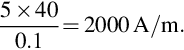
standing for Amperes) is the axial current per metre of circumference on the rotor. In a slotted rotor, the axial current is concentrated in the conductors within each slot, but to calculate ![]() we picture the total current to be spread uniformly over the circumference (in a manner similar to that shown in Fig. 1.13, but with the individual conductors under each pole being represented by a uniformly distributed ‘current sheet’). For example, if under a pole with a circumferential width of 10 cm we find that there are five slots, each carrying a current of 40 A, the electric loading is
we picture the total current to be spread uniformly over the circumference (in a manner similar to that shown in Fig. 1.13, but with the individual conductors under each pole being represented by a uniformly distributed ‘current sheet’). For example, if under a pole with a circumferential width of 10 cm we find that there are five slots, each carrying a current of 40 A, the electric loading is
The discussion in Section 1.4 referred to the conflicting demands of flux and current, so it should be clear that if we seek to increase the electric loading, for example by widening the slots to accommodate more copper, we must be aware that the magnetic loading may have to be reduced because the narrower teeth will mean there is less area for the flux, and therefore a danger of saturating the iron.
Many factors influence the values which can be employed in motor design, but in essence the specific magnetic and electric loadings are limited by the properties of the materials (iron for the flux, and copper for the current), and by the cooling system employed to remove heat losses.
The specific magnetic loading does not vary greatly from one machine to another, because the saturation properties of most core steels are similar, so there is an upper limit to the flux density that can be achieved. On the other hand, quite wide variations occur in the specific electric loadings, depending on the type of cooling used.
Despite the low resistivity of the copper conductors, heat is generated by the flow of current, and the current must therefore be limited to a value such that the insulation is not damaged by an excessive temperature rise. The more effective the cooling system, the higher the electric loading can be. For example, if the motor is totally enclosed and has no internal fan, the current density in the copper has to be much lower than in a similar motor which has a fan to provide a continuous flow of ventilating air. Similarly, windings which are fully impregnated with varnish can be worked much harder than those which are surrounded by air, because the solid body of encapsulating varnish not only gives mechanical rigidity but also provides a much better thermal path along which the heat can flow to the stator body. Overall size also plays a part in determining permissible electric loading, with larger motors generally having higher values than small ones.
In practice, the important point to be borne in mind is that unless an exotic cooling system is employed, most motors (induction, d.c., etc.) of a particular size have more or less the same specific loadings, regardless of type. As we will now see, this in turn means that motors of similar size have broadly similar torque capabilities, regardless of the specific motor type/technology. This fact is not widely appreciated by users, but is always worth bearing in mind.
1.5.2 Torque and rotor volume
In the light of the earlier discussion, we can obtain the total tangential force by first considering an area of the rotor surface of width w and length L. The axial current flowing in the width w is given by ![]() , and on average all of this current is exposed to radial flux density
, and on average all of this current is exposed to radial flux density ![]() so the tangential force is given (from Eq. 1.2) by
so the tangential force is given (from Eq. 1.2) by ![]() The area of the surface is wL so the force per unit area is
The area of the surface is wL so the force per unit area is ![]() . We see that the product of the two specific loadings expresses the average tangential stress over the rotor surface.
. We see that the product of the two specific loadings expresses the average tangential stress over the rotor surface.
To obtain the total tangential force we must multiply by the area of the curved surface of the rotor, and to obtain the total torque we multiply the total force by the radius of the rotor. Hence for a rotor of diameter D and length L, the total torque is given by
What this equation tells us is extremely important. The term D2L is proportional to the rotor volume, so we see that for given values of the specific magnetic and electric loadings, the torque from any motor is proportional to the rotor volume. We are at liberty to choose a long thin rotor or a short fat one, but once the rotor volume and specific loadings are specified, we have effectively determined the torque.
It is worth stressing that we have not focused on any particular type of motor, but have approached the question of torque production from a completely general viewpoint. In essence our conclusions reflect the fact that all motors are made from iron and copper, and differ only in the way these materials are disposed, and how hard they are worked.
We should also acknowledge that in practice it is the overall volume of the motor which is important, rather than the volume of the rotor. But again we find that, regardless of the type of motor, there is a fairly close relationship between the overall volume and the rotor volume, for motors of similar torque. We can therefore make the bold but generally accurate statement that the overall volume of a motor is determined by the torque it has to produce. There are of course exceptions to this rule, but as a general guideline for motor selection, it is extremely useful.
Having seen that torque depends on rotor volume, we must now turn our attention to the question of power output.
1.5.3 Output power—Importance of speed
Before deriving an expression for power a brief digression may be helpful for those who are more familiar with linear rather than rotary systems.
In the SI system, the unit of work or energy is the Joule (J). One Joule represents the work done by a force of 1 Newton moving 1 m in its own direction. Hence the work done (W) by a force F which moves a distance d is given by
With F in Newtons and d in metres, W is clearly in Newton-metres (Nm), from which we see that a Newton-metre is the same as a Joule.
In rotary systems, it is more convenient to work in terms of torque and angular distance, rather than force and linear distance, but these are closely linked as we can see by considering what happens when a tangential force F is applied at a radius r from the centre of rotation. The torque is simply given by
Now suppose that the arm turns through an angle θ, so that the circumferential distance travelled by the force is ![]() . The work done by the force is then given by
. The work done by the force is then given by
We note that whereas in a linear system work is force times distance, in rotary terms work is torque times angle. The units of torque are Newton-metres, and the angle is measured in radians (which is dimensionless), so the units of work done are Nm, or Joules, as expected. (The fact that torque and work (or energy) are measured in the same units does not seem self-evident to the authors!)
To find the power, or the rate of working, we divide the work done by the time taken. In a linear system, and assuming that the velocity remains constant, power is therefore given by
where v is the linear velocity. The angular equivalent of this is
where ![]() is the (constant) angular velocity, in radians per second.
is the (constant) angular velocity, in radians per second.
We can now express the power output in terms of the rotor dimensions and the specific loadings, using Eq. 1.9 which yields
Eq. (1.13) emphasises the importance of speed ![]() in determining power output. For given specific and magnetic loadings, if we want a motor of a given power we can choose between a large (and therefore expensive) low-speed motor or a small (and generally cheaper) high-speed one. The latter choice is preferred for most applications, even if some form of speed reduction (using belts or gears, for example) is needed, because the smaller motor is cheaper. Familiar examples include portable electric tools, where rotor speeds of 12,000 rev/min or more allow powers of hundreds of Watts to be obtained, and electric traction: in both the high motor speed is geared down for the final drive. In these examples, where volume and weight are at a premium, a direct drive would be out of the question.
in determining power output. For given specific and magnetic loadings, if we want a motor of a given power we can choose between a large (and therefore expensive) low-speed motor or a small (and generally cheaper) high-speed one. The latter choice is preferred for most applications, even if some form of speed reduction (using belts or gears, for example) is needed, because the smaller motor is cheaper. Familiar examples include portable electric tools, where rotor speeds of 12,000 rev/min or more allow powers of hundreds of Watts to be obtained, and electric traction: in both the high motor speed is geared down for the final drive. In these examples, where volume and weight are at a premium, a direct drive would be out of the question.
1.5.4 Power density (specific output power)
By dividing Eq. (1.13) by the rotor volume, we obtain an expression for the specific power output (power per unit rotor volume), Q, given by
The importance of this simple equation cannot be overemphasised. It is the fundamental design equation that governs the output of any ‘BIl’ machine, and thus applies to almost all motors.
To obtain the highest possible power from a given volume for given values of the specific magnetic and electric loadings, we must clearly operate the motor at the highest practicable speed. The one obvious disadvantage of a small high-speed motor and gearbox is that the acoustic noise (both from the motor itself and the from the power transmission) is higher than it would be from a larger direct drive motor. When noise must be minimised (for example in ceiling fans), a direct drive motor is therefore preferred, despite its larger size.
In this section, we began by exploring and quantifying the mechanism of torque production, so not surprisingly it was tacitly assumed that the rotor was at rest, with no work being done. We then moved on to assume that the torque was maintained when the speed was constant and useful power was delivered, i.e. that electrical energy was being converted into mechanical energy. The aim was to establish what factors determine the output of a rotor of given dimensions, and this was possible without reference to any particular type of motor.
In complete contrast, the approach in the next section focuses on a generic ‘primitive’ motor, and we begin to look in detail at what we have to do at the terminals in order to control the speed and torque.
1.6 Energy conversion—Motional e.m.f
We now examine the behaviour of a primitive linear machine which, despite its obvious simplicity, encapsulates all the key electromagnetic energy conversion processes that take place in electric motors. We will see how the process of conversion of energy from electrical to mechanical form is elegantly represented in an ‘equivalent circuit’ from which all the key aspects of motor behaviour can be predicted. This circuit will provide answers to such questions as ‘how does the motor automatically draw in more power when it is required to work’, and ‘what determines the steady speed and current’. Central to such questions is the matter of motional e.m.f., which is explored next.
We have already seen that force (and hence torque) is produced on current-carrying conductors exposed to a magnetic field. The force is given by Eq. (1.2), which shows that as long as the flux density and current remain constant, the force will be constant. In particular we see that the force does not depend on whether the conductor is stationary or moving. On the other hand relative movement is an essential requirement in the production of mechanical output power (as distinct from torque), and we have seen that output power is given by the equation P = Tω. We will now see that the presence of relative motion between the conductors and the field always brings ‘motional e.m.f.’ into play; and we will find that this motional e.m.f. plays a key role in quantifying the energy conversion process.
1.6.1 Elementary motor—Stationary conditions
The primitive linear machine is shown pictorially in Fig. 1.14 and in diagrammatic form in Fig. 1.15. It consists of a conductor of active1 length l which can move horizontally perpendicular to a magnetic flux density B.

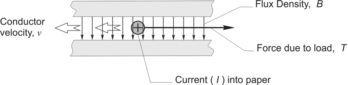
It is assumed that the conductor has a resistance (R), that it carries a d.c. current (I), and that it moves with a velocity (v) in a direction perpendicular to the field and the current (see Fig. 1.15). Attached to the conductor is a string which passes over a pulley and supports a weight: the tension in the string acting as a mechanical ‘load’ on the rod. Friction is assumed to be zero.
We need not worry about the many difficult practicalities of making such a machine, not least how we might manage to maintain electrical connections to a moving conductor. The important point is that although this is a hypothetical set-up, it represents what happens in a real motor, and it allows us to gain a clear understanding of how real machines behave before we come to grips with more complex structures.
We begin by considering the electrical input power with the conductor stationary (i.e. v = 0). For the purpose of this discussion we can suppose that the magnetic field (B) is provided by permanent magnets. Once the field has been established (when the magnet was first magnetised and placed in position), no further energy will be needed to sustain the field, which is just as well since it is obvious that an inert magnet is incapable of continuously supplying energy. It follows that when we obtain mechanical output from this primitive ‘motor’, none of the energy involved comes from the magnet. This is an extremely important point: the field system, whether provided from permanent magnets or ‘exciting’ windings, acts only as a catalyst in the energy conversion process, and contributes nothing to the mechanical output power.
When the conductor is held stationary the force produced on it (BIl) does no work, so there is no mechanical output power, and the only electrical input power required is that needed to drive the current through the conductor.
The resistance of the conductor is R, the current through it is I, so the voltage which must be applied to the ends of the rod from an external source will be given by ![]() and the electrical input power will be
and the electrical input power will be ![]() . Under these conditions, all the electrical input power will appear as heat inside the conductor, and the power balance can be expressed by the equation
. Under these conditions, all the electrical input power will appear as heat inside the conductor, and the power balance can be expressed by the equation
Although no work is being done because there is no movement, the stationary condition can only be sustained if there is equilibrium of forces. The tension in the string (T) must equal the gravitational force on the mass (mg), and this in turn must be balanced by the electromagnetic force on the conductor (BIl). Hence under stationary conditions the current must be given by
This is our first indication of the essential link that always exists (in the steady state) between the mechanical and electric worlds, because we see that in order to maintain the stationary condition, the current in the conductor is determined by the mass of the mechanical load. We will return to this interdependence later.
1.6.2 Power relationships—Conductor moving at constant speed
Now let us imagine the situation where the conductor is moving at a constant velocity (v) in the direction of the electromagnetic driving force that is propelling it. What current must there be in the conductor, and what voltage will have to be applied across its ends?
We start by recognising that constant velocity of the conductor means that the mass (m) is moving upwards at a constant speed, i.e. it is not accelerating. Hence from Newton’s law, there must be no resultant force acting on the mass, so the tension in the string (T) must equal the weight (mg).
Similarly, the conductor is not accelerating, so its net force must also be zero. The string is exerting a braking force (T), so the electromagnetic force (BIl) must be equal to T. Combining these conditions yields
This is exactly the same equation that we obtained under stationary conditions, and it underlines the fact that the steady-state current is determined by the mechanical load. When we develop the electrical equivalent circuit, we will have to get used to the idea that in the steady-state one of the electrical variables (the current) is determined by the mechanical load.
With the mass rising at a constant rate, mechanical work is being done because the potential energy of the mass is increasing. This work is coming from the moving conductor. The mechanical output power is equal to the rate of work, i.e. the force (T = BIl) times the velocity (v). The power lost as heat in the conductor is the same as it was when stationary, since it has the same resistance, and the same current. The electrical input power supplied to the conductor must continue to furnish this heat loss, but in addition it must now supply the mechanical output power. As yet we do not know what voltage will have to be applied, so we will denote it by V2. The power balance equation now becomes

We note that the first term on the right hand side of Eq. (1.18) represents the heating effect, which is the same as when the conductor was stationary, while the second term corresponds to the additional power that must be supplied to provide the mechanical output. Since the current is the same but the input power is now greater, the new voltage ![]() must be higher than
must be higher than ![]() .
.
By subtracting Eq. (1.15) from Eq. (1.18) we obtain
and thus
Eq. (1.19) quantifies the extra voltage to be provided by the source to keep the current constant when the conductor is moving. This increase in source voltage is a reflection of the fact that whenever a conductor moves through a magnetic field, an electromotive force or voltage (E) is induced in it.
We see from Eq. (1.19) that the e.m.f. is directly proportional to the flux density, to the velocity of the conductor relative to the flux, and to the active length of the conductor. The source voltage has to overcome this additional voltage in order to keep the same current flowing: if the source voltage was not increased, the current would fall as soon as the conductor began to move because of the opposing effect of the induced e.m.f.
We have deduced that there must be an e.m.f. caused by the motion, and have derived an expression for it by using the principle of the conservation of energy, but the result we have obtained, i.e.
is often introduced as the ‘flux-cutting’ form of Faraday’s law, which states that when a conductor moves through a magnetic field an e.m.f., given by Eq. (1.20), is induced in it. Because motion is an essential part of this mechanism, the e.m.f. induced is often referred to as a ‘motional e.m.f.’. The ‘flux-cutting’ terminology arises from attributing the origin of the e.m.f. to the cutting or slicing of the lines of flux by the passage of the conductor. This is a useful mental picture, though it must not be pushed too far: after all the flux lines are merely inventions which we find helpful in coming to grips with magnetic matters.
Before turning to the equivalent circuit of the primitive motor two general points are worth noting. Firstly, whenever energy is being converted from electrical to mechanical form, as here, the induced e.m.f. always acts in opposition to the applied (source) voltage. This is reflected in the use of the term ‘back e.m.f.’ to describe motional e.m.f. in motors. Secondly, although we have discussed a particular situation in which the conductor carries current, it is certainly not necessary for any current to be flowing in order to produce an e.m.f.: all that is needed is relative motion between the conductor and the magnetic field.
1.7 Equivalent circuit
We can represent the electrical relationships in the primitive machine in an equivalent circuit as shown in Fig. 1.16.

The resistance of the conductor and the motional e.m.f. together represent in circuit terms what is happening in the conductor (though in reality the e.m.f. and the resistance are distributed, not lumped as separate items). The externally applied source that drives the current is represented by the voltage V on the left (the old-fashioned battery symbol being deliberately used to differentiate the applied voltage V from the induced e.m.f. E). We note that the induced motional e.m.f. is shown as opposing the applied voltage, which applies in the ‘motoring’ condition we have been discussing. Applying Kirchoff’s law we obtain the voltage equation as
Multiplying Eq. (1.21) by the current gives the power equation as

(Note that the term ‘copper loss’ used in Eq. (1.22) refers to the heat generated by the current in the windings: all such losses in electric motors are referred to in this way, even when the conductors are made of aluminium or bronze!)
It is worth seeing what can be learned from these equations because, as noted earlier, this simple elementary ‘motor’ encapsulates all the essential features of real motors. Lessons which emerge at this stage will be invaluable later, when we look at the way actual motors behave.
1.7.1 Motoring and generating
If the e.m.f. E is less than the applied voltage V, the current will be positive, and electrical power will flow from the source, resulting in motoring action in which energy is converted from electrical to mechanical form. The first term on the right hand side of Eq. (1.22), which is the product of the motional e.m.f. and the current, represents the mechanical output power developed by the primitive linear motor, but the same simple and elegant result applies to real motors. We may sometimes have to be a bit careful if the e.m.f. and the current are not simple d.c. quantities, but the basic idea will always hold good.
Now let us imagine that we push the conductor along at a steady speed that makes the motional e.m.f. greater than the applied voltage. We can see from the equivalent circuit that the current will now be negative (i.e. anticlockwise), flowing back into the supply and thus returning energy to the supply. And if we look at Eq. (1.22), we see that with a negative current, the first term (-VI) represents the power being returned to the source, the second term (-EI) corresponds to the mechanical power being supplied by us pushing the rod along, and the third term is the heat loss in the conductor.
For readers who prefer to argue from the mechanical standpoint, rather than the equivalent circuit, we can say that when we are generating a negative current (− I), the electromagnetic force on the conductor is (− BIl), i.e. it is directed in the opposite direction to the motion. The mechanical power is given by the product of force and velocity, i.e. (− BIlv), or − EI, as above.
The fact that exactly the same kit has the inherent ability to switch from motoring to generating without any interference by the user is an extremely desirable property of all electromagnetic energy converters. Our primitive set-up is simply a machine which is equally at home acting as a motor or a generator.
Finally, it is obvious that in a motor we want as much as possible of the electrical input power to be converted to mechanical output power, and as little as possible to be converted to heat in the conductor. Since the output power is EI, and the heat loss is ![]() , we see that ideally we want EI to be much greater than
, we see that ideally we want EI to be much greater than ![]() , or in other words E should be much greater than IR. In the equivalent circuit (Fig. 1.16) this means that the majority of the applied voltage V is accounted for by the motional e.m.f. (E), and only a little of the applied voltage is used in overcoming the resistance.
, or in other words E should be much greater than IR. In the equivalent circuit (Fig. 1.16) this means that the majority of the applied voltage V is accounted for by the motional e.m.f. (E), and only a little of the applied voltage is used in overcoming the resistance.
1.8 Constant voltage operation
Up to now, we have studied behaviour under ‘steady-state’ conditions, which in the context of motors means that the load is constant and conditions have settled to a steady speed. We saw that with a constant load, the current was the same at all steady speeds, the voltage being increased with speed to take account of the rising motional e.m.f. This was a helpful approach to take in order to illuminate the energy conversion process, but is seldom typical of normal operation. We therefore turn to how the moving conductor will behave under conditions where the applied voltage V is constant, since this corresponds more closely with normal operation of a real motor.
Matters inevitably become more complicated because we consider how the motor gets from one speed to another, as well as what happens under steady-state conditions. As in all areas of dynamics, study of the transient behaviour of our primitive linear motor brings into play additional parameters such as the mass of the conductor (equivalent to the inertia of a rotary motor) which are absent from steady-state considerations.
1.8.1 Behaviour with no mechanical load
In this section we assume that the hanging weight has been removed, and that the only force on the conductor is its own electromagnetically generated one. Our primary interest will be in what determines the steady speed of the primitive motor, but we begin by considering what happens when we first apply the voltage.
With the conductor stationary when the voltage V is applied, there is no motional e.m.f. and the current will immediately rise to a value of V/R, since the only thing which limits the current is the resistance. (Strictly we should allow for the effect of inductance in delaying the rise of current, but we choose to ignore it here in the interests of simplicity.) The resistance will be small, so the current will be large, and a high ‘BIl’ force will therefore be developed on the conductor. The conductor will therefore accelerate at a rate governed by Newton’s law, i.e. acceleration = the force acting on it divided by its mass.
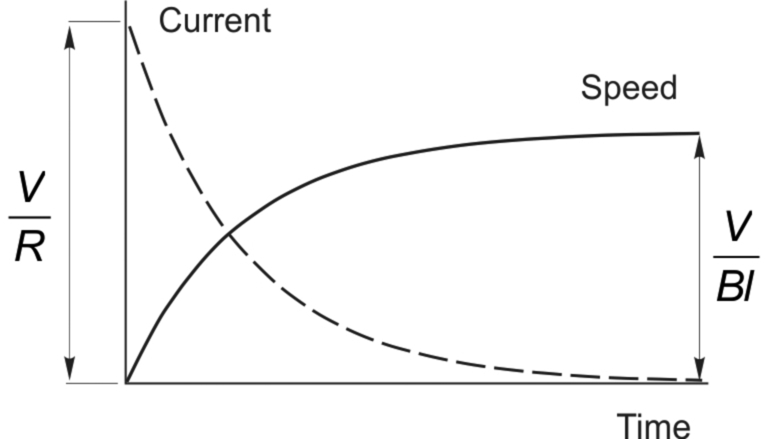
As the speed (v) increases, the motional e.m.f. (Eq. 1.20) will grow in proportion to the speed. Since the motional e.m.f. opposes the applied voltage, the current will fall (Eq. 1.21), so the force and hence the acceleration will reduce, though the speed will continue to rise. The speed will increase as long as there is an accelerating force, i.e. as long as there is a current in the conductor. We can see from Eq. (1.21) that the current will finally fall to zero when the speed reaches a level at which the motional e.m.f. is equal to the applied voltage. The speed and current therefore vary as shown in Fig. 1.17, both curves having the exponential shape which characterises the response of systems governed by a first-order differential equation. The fact that the steady-state current is zero is in line with our earlier observation that the mechanical load (in this case zero) determines the steady-state current.
We note that in this idealised situation (in which there is no load applied, and no friction forces), the conductor will continue to travel at a constant speed, because with no net force acting on it there is no acceleration. Of course, no mechanical power is being produced, since we have assumed that there is no opposing force on the conductor, and there is no input power because the current is zero. This hypothetical situation nevertheless corresponds closely to the so-called ‘no-load’ condition in a motor, the only difference being that a motor will have some friction (and therefore it will draw a small current), whereas we have assumed no friction in order to simplify the discussion.
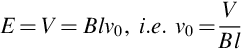
An elegant self-regulating mechanism is evidently at work here. When the conductor is stationary, it has a high force acting on it, but this force tapers-off as the speed rises to its target value, which corresponds to the back e.m.f. being equal to the applied voltage. Looking back at the expression for motional e.m.f. (Eq. 1.18), we can obtain an expression for the no-load speed v0 by equating the applied voltage and the back e.m.f., which gives
Eq. (1.23) shows that the steady-state no-load speed is directly proportional to the applied voltage, which indicates that speed control can be achieved by means of the applied voltage. We will see later that one of the main reasons why d.c. motors held sway in the speed-control arena for so long is that their speed can be controlled via the applied voltage.
Rather more surprisingly, Eq. (1.23) reveals that the speed is inversely proportional to the magnetic flux density, which means that the weaker the field, the higher the steady-state speed. This result can cause raised eyebrows, and with good reason. Surely, it is argued, since the force is produced by the action of the field, the conductor will not go as fast if the field is weaker. This view is wrong, but understandable.
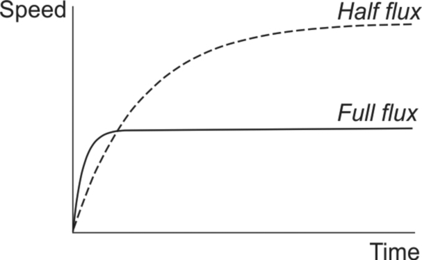
The flaw in the argument is to equate force with speed. When the voltage is first applied, the force on the conductor certainly will be less if the field is weaker, and the initial acceleration will be lower. But in both cases the acceleration will continue until the current has fallen to zero, and this will only happen when the induced e.m.f. has risen to equal the applied voltage. With a weaker field, the speed needed to generate this e.m.f. will be higher than with a strong field: there is ‘less flux’, so what there is has to be cut at a higher speed to generate a given e.m.f. The matter is summarised in Fig. 1.18, which shows how the speed will rise for a given applied voltage, for ‘full’ and ‘half’ fields respectively. Note that the initial acceleration (i.e. the slope of the speed-time curve) in the half-flux case is half that of the full flux case, but the final steady speed is twice as high. In motors the technique of reducing the flux density in order to increase speed is known as ‘field weakening’.
1.8.2 Behaviour with a mechanical load
Suppose that, with the primitive linear motor up to its no-load speed we suddenly attach the string carrying the weight, so that we now have a steady force T (= mg), opposing the motion of the conductor. At this stage there is no current in the conductor and thus the only force on it will be T. The conductor will therefore begin to decelerate. But as soon as the speed falls, the back e.m.f. will become less than V, and current will begin to flow into the conductor, producing an electromagnetic driving force. The more the speed drops, the bigger the current, and hence the larger the force developed by the conductor. When the force developed by the conductor becomes equal to the load (T), the deceleration will cease, and a new equilibrium condition will be reached. The speed will be lower than at no-load, and the conductor will now be producing continuous mechanical output power, i.e. acting as a motor.
We recall that the electromagnetic force on the conductor is directly proportional to the current, so it follows that the steady-state current is directly proportional to the load which is applied, as we saw earlier. If we were to explore the transient behaviour mathematically, we would find that the drop in speed followed the same first-order exponential response that we saw in the run-up period. Once again the self-regulating property is evident, in that when load is applied the speed drops just enough to allow sufficient current to flow to produce the force required to balance the load. We could hardly wish for anything better in terms of performance, yet the conductor does it without any external intervention on our part.
(Readers who are familiar with closed-loop control systems will probably recognise that the reason for this excellent performance is that the primitive motor possesses inherent negative speed feedback via the motional e.m.f.).
Returning to Eq. (1.21), we note that the current depends directly on the difference between V and E, and inversely on the resistance. Hence for a given resistance, the larger the load (and hence the steady-state current), the greater the required difference between V and E, and hence the lower the steady running speed, as shown in Fig. 1.19.
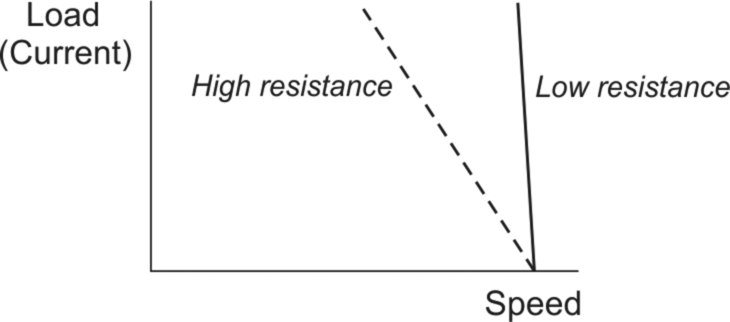
We can also see from Eq. (1.21) that the higher the resistance of the conductor, the more it slows down when a given load is applied. Conversely, the lower the resistance, the more the conductor is able to hold its no-load speed in the face of applied load, as also shown in Fig. 1.19. We can deduce that the only way we could obtain an absolutely constant speed with this type of motor is for the resistance of the conductor to be zero, which is of course not possible. Nevertheless, real d.c. motors generally have resistances which are small, and their speed does not fall much when load is applied—a characteristic which is highly desirable for most applications.
We complete our exploration of the performance when loaded by asking how the flux density influences behaviour. Recalling that the electromagnetic force is proportional to the flux density as well as the current, we can deduce that to develop a given force, the current required will be higher with a weak flux than with a strong one. Hence in view of the fact that there will always be an upper limit to the current which the conductor can safely carry, the maximum force which can be developed will vary in direct proportion to the flux density, with a weak flux leading to a low maximum force and vice-versa. This underlines the importance of operating with maximum flux density whenever possible.
We can also see another disadvantage of having a low flux density by noting that to achieve a given force, the drop in speed will be disproportionately high when we go to a lower flux density. We can see this by imagining that we want a particular force, and considering how we achieve it firstly with full flux, and secondly with half flux. With full flux, there will be a certain drop in speed which causes the motional e.m.f. to fall enough to admit the required current. But with half the flux, for example, twice as much current will be needed to develop the same force. Hence the motional e.m.f. must fall by twice as much as it did with full flux. However, since the flux density is now only half, the drop in speed will have to be four times as great as it was with full flux. The half-flux ‘motor’ therefore has a load characteristic with a load/speed gradient four times more droopy than the full-flux one. This is shown in Fig. 1.20 the applied voltages having been adjusted so that in both cases the no-load speed is the same. The half-flux motor is clearly inferior in terms of its ability to hold the set speed when the load is applied.
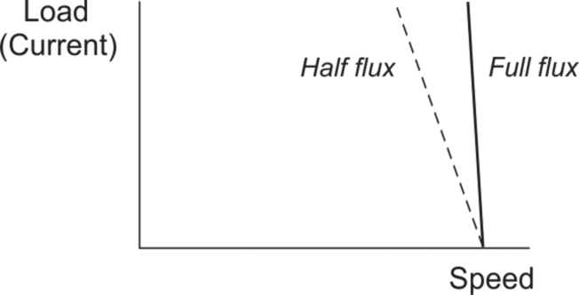
We may have been tempted to think that the higher speed which we can obtain by reducing the flux somehow makes for better performance, but we can now see that this is not so. By halving the flux, for example, the no load speed for a given voltage is doubled, but when the load is raised until rated current is flowing in the conductor, the force developed is only half, so the mechanical power is the same. We are in effect trading speed against force, and there is no suggestion of getting something for nothing.
1.8.3 Relative magnitudes of V and E, and efficiency
Invariably we want machines which have high efficiency. From Eq. (1.20), we see that to achieve high efficiency, the copper loss (I2R) must be small compared with the mechanical power (EI), which means that the resistive volt-drop in the conductor (IR) must be small compared with either the induced e.m.f. (E) or the applied voltage (V). In other words we want most of the applied voltage to be accounted for by the ‘useful’ motional e.m.f., rather than the wasteful volt drop in the wire. Since the motional e.m.f. is proportional to speed, and the resistive volt drop depends on the conductor resistance, we see that a good energy converter requires the conductor resistance to be as low as possible, and the speed to be as high as possible.
To provide a feel for the sorts of numbers likely to be encountered, we can consider a conductor with resistance of 0.5 Ω, capable of carrying a current of 4 A without overheating, and moving at a speed such that the motional e.m.f. is 8 V. From Eq. (1.19), the supply voltage is given by
Hence the electrical input power (VI) is 40 W, the mechanical output power (EI) is 32 W, and the copper loss (I2R) is 8 W, giving an efficiency of 80%.
If the supply voltage was doubled (i.e. V = 20 Volts), however, and the resisting force is assumed to remain the same (so that the steady-state current is still 4 A), the motional e.m.f. is given by Eq. (1.21) as
which shows that the speed will have more than doubled, as expected. The electrical input power is now 80 W, the mechanical output power is 72 W, and the copper loss is still 8 W. The efficiency has now risen to 90%, underlining the fact that the energy conversion process gets better at higher speeds.
When we operate the machine as a generator, we again benefit from the higher speeds. For example, with the battery voltage maintained at 10 V, and the conductor being propelled by an external force so that its e.m.f. was 12 V, the allowable current of 4 A would now be flowing into the battery, with energy being converted from mechanical to electrical form. The power into the battery (VI) is 40 W, the mechanical input power (EI) is 48 W and the heat loss 8 W. In this case efficiency is defined as the ratio of useful electrical power divided by mechanical input power, i.e. 40/48, or 83.3%.
If we double the battery voltage to 20 V and increase the driven speed so that the motional e.m.f. rises to 22 V, we will again supply the battery with 4 A, but the efficiency will now be 80/88, or 90.9%.
The ideal situation is clearly one where the term IR in Eq. (1.22) is negligible, so that the back e.m.f. is equal to the applied voltage. We would then have an ideal machine with an efficiency of 100%, in which the steady-state speed would be directly proportional to the applied voltage and independent of the load.
In practice the extent to which we can approach the ideal situation discussed above depends on the size of the machine. Tiny motors, such as those used in wrist watches, are awful, in that most of the applied voltage is used up in overcoming the resistance of the conductors, and the motional e.m.f. is very small: these motors are much better at producing heat than they are at producing mechanical output power! Small machines, such as those used in hand tools, are a good deal better with the motional e.m.f. accounting for perhaps 70–80% of the applied voltage. Industrial machines are very much better: the largest ones (of many hundreds of kW) use only 1 or 2% of the applied voltage in overcoming resistance, and therefore have very high efficiencies.
1.8.4 Analysis of primitive machine—Conclusions
All of the lessons learned from looking at the primitive machine will find direct parallels in almost all of the motors we look at in the rest of this book, so it is worth reminding ourselves of the key points.
Although this book is primarily about motors, perhaps the most important conclusion so far is that electrical machines are inherently bi-directional energy converters, and any motor can be made to generate, or vice-versa. We also saw that the efficiency of the energy-conversion process improves at high speeds, which explains why direct-drive slow-speed motors are not widely used.
In terms of the theoretical underpinning, we will make frequent reference to the formula for the force on a conductor in a magnetic field, i.e.
and to the formula for the motional induced e.m.f, i.e.
where B is the magnetic flux density, I is the current, l is the length of conductor and v is the velocity perpendicular to the field.
Specifically in relation to d.c. machines, we have seen that the speed at which the primitive motor runs unloaded is determined by the applied voltage, while the steady-state current that the motor draws is determined by the mechanical load. Exactly the same results will hold when we examine real d.c. motors, and very similar relationships will also emerge when we look at a.c. machines.
1.9 General properties of electric motors
All electric motors are governed by the laws of electromagnetism, and are subject to essentially the same constraints imposed by the materials (copper or aluminium for the electric circuit, magnetic steel, and insulation) from which they are made. We should therefore not be surprised to find that, at the fundamental level, all motors—regardless of type—have a great deal in common.
These common properties, most of which have been touched on in this chapter, are not usually given prominence. Books tend to concentrate on the differences between types of motor, and manufacturers are usually interested in promoting the virtues of their particular motor at the expense of the competition. This divisive emphasis can cause the underlying unity to be obscured, leaving users with little opportunity to absorb the sort of knowledge which will equip them to make informed judgements.
The most useful ideas worth bearing in mind are therefore given below, with brief notes accompanying each. Experience indicates that users who have these basic ideas firmly in mind will find themselves better able to understand why one motor is better than another, and will feel more confident when faced with the difficult task of weighing the pros and cons of competing types.
1.9.1 Operating temperature and cooling
The cooling arrangement is the single most important factor in determining the permissible output from any given motor.
Any motor will give out more power if its electric circuit is worked harder (i.e. if the current is allowed to increase). The limiting factor is normally the allowable temperature rise of the windings, which depends on the class of insulation.
For class F insulation (the most widely used) the permissible temperature rise is 100 K, whereas for class H it is 125 K. Thus if the cooling remains the same, more output can be obtained simply by using the higher-grade insulation. Alternatively, with a given insulation the output can be increased if the cooling system is improved. A through-ventilated motor, for example, might give perhaps twice the output power of an otherwise identical but totally enclosed machine.
1.9.2 Torque per unit volume
For motors with similar cooling systems, the rated torque is approximately proportional to the rotor volume, which in turn is roughly proportional to the overall motor volume.
This stems from the fact that for a given cooling arrangement, the electric and magnetic loadings of machines of different types will be more or less the same. The torque per unit length therefore depends first and foremost on the square of the diameter, so motors of roughly the same diameter and length can be expected to produce roughly the same torque.
1.9.3 Power per unit volume and efficiency—Importance of speed
Output power per unit volume is directly proportional to speed.
Low-speed motors are unattractive for most applications because they are large, and therefore expensive. It is usually better to use a high-speed motor with mechanical speed reduction. For example, a direct drive motor for a portable electric screwdriver would be an absurd proposition. On the other hand the reliability and inefficiency of gearboxes may sometimes outweigh the size argument, especially in high-power applications.
The efficiency of a motor improves with speed.
For a given torque, power output usually rises in direct proportion to speed, while electrical losses tend to rise less rapidly, so that efficiency rises with speed.
1.9.4 Size effects—Specific torque and efficiency
Large motors have a higher specific torque (torque per unit volume) and are more efficient than small ones.
In large motors the specific electric loading is normally much higher than in small ones, and the specific magnetic loading is somewhat higher. These two factors combine to give the higher specific torque.
Very small motors are inherently very inefficient (e.g. 1% in a wrist-watch), whereas motors of over say 100 kW have efficiencies above 96%. The reasons for this scale effect are complex, but stem from the fact that the resistance volt-drop term can be made relatively small in large electromagnetic devices, whereas in small ones the resistance becomes the dominant term.
1.9.5 Rated voltage
A motor can be provided to suit any voltage.
Within limits it is possible to rewind a motor for a different voltage without affecting its performance. A 200 V, 10 A motor could be rewound for 100 V, 20 A simply by using half as many turns per coil of wire having twice the cross-sectional area, the m.m.f. remaining the same. The total amounts of active material, and hence the performance, would be the same. This argument breaks down if pushed too far of course: a very small motor originally wound for 100 V would almost certainly require a larger frame if required to operate at 690 V, because of the additional space required for the higher-grade insulation.
1.9.6 Short-term overload
Most motors can be overloaded for short periods without damage.
The continuous electric loading (i.e. the current) cannot be exceeded without overheating and damaging the insulation, but if the motor has been running with reduced current for some time, it is permissible for the current (and hence the torque) to be much greater than normal for a short period of time. The principal factors which influence the magnitude and duration of the permissible overload are the thermal time-constant (which governs the rate of rise of temperature) and the previous pattern of operation. Thermal time constants range from a few seconds for small motors to many minutes or even hours for large ones. Operating patterns are obviously very variable, so rather than rely on a particular pattern being followed, it is usual for motors to be provided with over-temperature protective devices (e.g. thermistors) which trigger an alarm and/or trip the supply if the safe temperature is exceeded.
Motors can of course be designed for specific applications with known duty cycles, where the thermal and electric loading can be accommodated. This is discussed further in Chapter 11.
1.10 Review questions
- (1) The current in a coil with 250 turns is 8 A. Calculate the m.m.f.
- (2) The coil in Q1 is used in a magnetic circuit with a uniform cross-section made of good-quality magnetic steel and with a 2 mm air-gap. Estimate the flux density in the air-gap, and in the iron. (μ0 = 4 × 10− 7 Hm− 1)
How would the answers change if the cross-sectional area of the magnetic circuit was doubled, with all other parameters remaining the same? - (3) A magnetic circuit of uniform cross-sectional area has two air-gaps of 0.5 and 1 mm respectively in series. The exciting winding provides an m.m.f. of 1200 Amp-turns. Estimate the m.m.f. across each of the air-gaps, and the flux density.
- (4) The rotor of a d.c. motor had an original diameter of 30 cm and an air-gap under the poles of 2 mm. During refurbishment the rotor diameter was accidentally reground and was then undersize by 0.5 mm. Estimate by how much the field m.m.f. would have to be increased to restore normal performance. How might the extra m.m.f. be provided?
- (5) Calculate the electromagnetic force on:
- (a) a single conductor of length 25 cm, carrying a current of 4A, exposed to a magnetic flux density of 0.8 T perpendicular to its length.
- (b) a coil-side consisting of 20 wires of length 25 cm, each carrying a current of 2 A, exposed to a magnetic flux density of 0.8 T perpendicular to its length.
- (6) Estimate the torque produced by one of the early machines illustrated in Fig. 1.12 given the following:- Mean air-gap flux density under pole-face = 0.4 T; pole-arc as a percentage of total circumference = 75%; active length of rotor = 50 cm; rotor diameter = 30 cm; inner diameter of stator pole = 32 cm; total number of rotor conductors = 120; current in each rotor conductor = 50 A.
- (7) If the field coils of a motor are rewound to operate from 220 V instead of 110 V, how will the new winding compare with the old in terms of number of turns, wire diameter, power consumption and physical size?
- (8) A catalogue of DIY power tools indicates that most of them are available in 240 V or 110 V versions. What differences would you expect in terms of appearance, size, weight and performance?
- (9) Given that the field windings of a motor do not contribute to the mechanical output power, why do they consume power continuously?
- (10) Explain briefly why low-speed electrical drives often employ a high-speed motor and some form of mechanical speed reduction, rather than a direct-drive motor.
Answers to the review questions are given in the Appendix.