Stepping and switched reluctance motors
Abstract
The key features that link the relatively small stepping motor with the much larger switched reluctance (SR) motor are that they have salient poles on both rotor and stator; the torque-producing mechanism is the same for both; and they only became practicable with the arrival of power electronics. The difference is that the stepping motor is used primarily for low-power open-loop position control, while the SR drive competes in the medium power industrial drive area. The descriptive and graphical approach in this chapter reflects the lack of an easy analytical treatment of doubly salient machines, but nevertheless provides a grasp of the essential performance and design constraints for these drive types.
Keywords
Salient poles; Stepping motor; Hybrid motor; Open-loop; Closed-loop; Step angle; Pull-out torque; Switched reluctance motor
10.1 Introduction
We have grouped stepping and switched reluctance (SR) motors because despite substantial differences between the modes of operation (and the power ratings), the fundamental mechanism, i.e. reluctance torque, is the same in both. However, unlike the (synchronous) reluctance motors considered in Chapter 9, stepping and switched reluctance motors are ‘doubly-salient’ with projecting poles or saliencies on both the stator and the rotor (see Fig. 10.5).
In Chapter 9 we explained that reluctance torque referred to the natural tendency of the projecting poles on a rotor (without any windings or magnets) to align themselves with the axes of the multi-polar field produced by the windings on the smooth stator. Intuitively, therefore, it should not be difficult to see that the reluctance torque is further enhanced when we replace the smooth bore stator by one with projecting poles carrying discrete exciting windings. In effect, we are ‘sharpening up the focus’ of the stator field, and thus increasing the stiffness of the rotor about its equilibrium alignment position.
We will see that doubly salient machines require their discrete stator windings to be switched sequentially across a d.c. supply, and it was the difficulty of doing this that proved the stumbling block for the early nineteenth century pioneers, who saw these inherently simple machines as being suitable for electric traction. The mechanical switching devices at the time were inadequate, and it was not until power semiconductor devices arrived in the 1960s that interest in the technology was renewed.
The theoretical treatment of doubly-salient machines is not as straightforward as that for motors with smooth stators and rotors such as the induction motor or the non-salient synchronous motor, which we have studied in previous chapters. For those motors it was relatively easy to explain the mechanism of torque production using the ‘force on a conductor' formula (‘BIl'), and because the windings were sinusoidally distributed in space, and the currents were sinusoidal in time, we were able to make extensive use of space and time phasors to illuminate performance. We even managed to explain and quantify reluctance torque in a singly-salient motor by the same approach.
Unfortunately the ‘BIl' approach does not lend itself easily to the analysis of doubly-salient machines. Instead, most analysis and design is based on computer-aided modelling of the complex flux patterns (often involving high levels of saturation), in order to establish how the flux linking each winding varies with the position of the rotor and the currents in the windings. The torque is then predicted using the circuit-based approach outlined in Section 3.4 of Chapter 8. As a result there are few if any analytic results that are helpful in terms of understanding, and we will therefore follow a largely descriptive approach in this chapter, beginning with stepping motors because they provide useful groundwork for the SR material that follows.
10.2 Stepping motors
Stepping (or stepper) motors historically became attractive because they can be controlled directly by computers, microcontrollers and Programmable Logic Controllers (PLC's).1 Their unique feature is that the output shaft rotates in a series of discrete angular intervals, or steps, one step being taken each time a command pulse is received. When a definite number of pulses has been supplied, the shaft will have turned through a known angle, and this makes the motor well suited for open-loop position control.
The idea of a shaft progressing in a series of steps might conjure up visions of a ponderous device laboriously indexing until the target number of steps has been reached, but this would be quite wrong. Each step is completed very quickly, often in less than a millisecond; and when a large number of steps is called for the step command pulses can be delivered rapidly, sometimes as fast as several thousand steps per second. At these high stepping rates the shaft rotation becomes smooth, and the behaviour resembles that of an ordinary motor. Typical applications include disc head drives, and small numerically-controlled machine tool slides, where the motor would drive a lead screw; and print feeds, where the motor might drive directly, or via a belt.
Most stepping motors look much like conventional motors, and as a general guide we can assume that the torque and power of a stepping motor will be similar to the torque and power of a conventional totally-enclosed motor of the same dimensions and speed range. Step angles are mostly in the range 1.8–90°, with torques ranging from 1 μNm (in a tiny wristwatch motor of 3 mm diameter) up to perhaps 40 Nm in a motor of 15 cm diameter suitable for a machine tool application where speeds of 500 rev/min might be called for, but the majority of applications use motors which can be held comfortably in the hand.
10.2.1 Open-loop position control
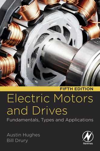
A basic stepping motor system is shown in Fig. 10.1.
The drive contains the electronic switching circuits which supply the motor, and is discussed later. The output is the angular position of the motor shaft, while the input consists of two low-power digital signals. Every time a pulse occurs on the step input line, the motor takes one step, the shaft remaining at its new position until the next step pulse is supplied. The state of the direction line (‘high’ or ‘low’) determines whether the motor steps clockwise or anticlockwise. A given number of step pulses will therefore cause the output shaft to rotate through a definite angle.
This one to one correspondence between pulses and steps is the great attraction of the stepping motor: it provides position control, because the output is the angular position of the output shaft. It is a digital system, because the total angle turned through is determined by the number of pulses supplied; and it is open-loop because no feedback need be taken from the output shaft.
10.2.2 Generation of step pulses and motor response
The step pulses may be produced by a digital controller or microprocessor (or even an oscillator controlled by an analogue voltage). When a given number of steps is to be taken, the step pulses are gated to the drive and the pulses are counted, until the required number of steps is reached, when the pulse train is gated off. This is illustrated in Fig. 10.2, for a six-step sequence. There are six step command pulses, equally spaced in time, and the motor takes one step following each pulse.

Three important general features can be identified with reference to Fig. 10.2. Firstly, although the total angle turned through (6 steps) is governed only by the number of pulses, the average speed of the shaft (which is shown by the slope of the broken line in Fig. 10.2) depends on the frequency. The higher the frequency, the shorter the time taken to complete the six steps.
Secondly, the stepping action is not perfect. The rotor takes a finite time to move from one position to the next, and then overshoots and oscillates before finally coming to rest at the new position. Overall single-step times vary with motor size, step angle and the nature of the load, but are commonly within the range 5–100 ms. This is often fast enough not to be seen by the unwary newcomer, though individual steps can usually be heard; small motors ‘tick’ when they step, and larger ones make a satisfying ‘click’ or ‘clunk’.
Thirdly, in order to be sure of the absolute position at the end of a stepping sequence, we must know the absolute position at the beginning. This is because a stepping motor is an incremental device. As long as it is not abused, it will always take one step when a drive pulse is supplied, but in order to keep track of absolute position simply by counting the number of drive pulses (and this is after all the main virtue of the system) we must always start the count from a known datum position. Normally the step counter will be ‘zeroed’ with the motor shaft at the datum position, and will then count up for clockwise direction, and down for anticlockwise rotation. Provided no steps are lost (see later) the number in the step counter will then always indicate the absolute position.
10.2.3 High speed running and ramping
The discussion so far has been restricted to operation when the step command pulses are supplied at a constant rate, and with sufficiently long intervals between the pulses to allow the rotor to come to rest between steps. Very large numbers of small stepping motors in watches and clocks do operate continuously in this way, stepping perhaps once every second, but most commercial and industrial applications call for a more exacting and varied performance.
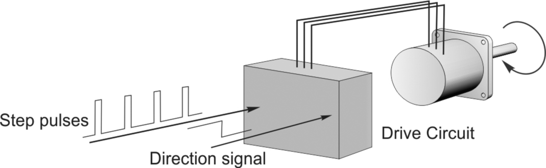
To illustrate the variety of operations which might be involved, and to introduce high-speed running, we can look briefly at a typical industrial application. A stepping motor-driven table feed on a numerically-controlled milling machine nicely illustrates both of the key operational features discussed earlier. These are the ability to control position (by supplying the desired number of steps) and velocity (by controlling the stepping rate).
The arrangement is shown diagrammatically in Fig. 10.3. The motor turns a leadscrew connected to the worktable, so that each motor step causes a precise incremental movement of the workpiece relative to the cutting tool. By making the increment small enough, the fact that the motion is discrete rather than continuous will not cause any difficulties in the machining process in most applications. We will assume that we have selected the step angle, the pitch of the leadscrew, and any necessary gearing so as to give a table movement of 0.01 mm per motor step. We will also assume that the necessary step command pulses will be generated by a digital controller or computer, programmed to supply the right number of pulses, at the right speed for the work in hand.
If the machine is a general-purpose one, many different operations will be required. When taking heavy cuts, or working with hard material, the work will have to be offered to the cutting tool slowly, at say, 0.02 mm/s. The stepping rate will then have to be set to 2 steps/s. If we wish to mill out a slot 1 cm long, we will therefore programme the controller to put out 1000 steps, at a uniform rate of 2 steps/s, and then stop. On the other hand, the cutting speed in softer material could be much higher, with stepping rates in the range 10–100 steps/s being in order. At the completion of a cut, it will be necessary to traverse the work back to its original position, before starting another cut. This operation needs to be done as quickly as possible to minimise unproductive time, and a stepping rate of perhaps 2000 steps/s (or even higher), may be called for.
It was mentioned earlier that a single step (from rest) takes upwards of several milliseconds. It should therefore be clear that if the motor is to run at 2000 steps/s (i.e. 0.5 ms/step), it cannot possibly come to rest between successive steps, as it does at low stepping rates. Instead, we find in practice that at these high stepping rates, the rotor velocity becomes quite smooth, with hardly any outward hint of its stepwise origins. Nevertheless, the vital one-to-one correspondence between step command pulses and steps taken by the motor is maintained throughout, and the open-loop position control feature is preserved. This extraordinary ability to operate at very high stepping rates (e.g. at 20,000 steps/s), and yet to remain in synchronism with the command pulses, is the most striking feature of stepping motor systems.
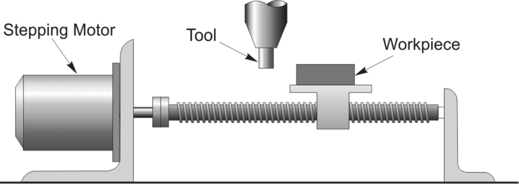
Operation at high speeds is referred to as ‘slewing’. The transition from single-stepping (as shown in Fig. 10.2) to high-speed slewing is a gradual one and is indicated by the sketches in Fig. 10.4. Roughly speaking, the motor will ‘slew’ if its stepping rate is above the frequency of its single-step oscillations. When motors are in the slewing range, they generally emit an audible whine, with a fundamental frequency equal to the stepping rate.
Naturally, a motor cannot be started from rest and expected to ‘lock on’ directly to a train of command pulses at, say, 2000 steps/s, which is well into the slewing range. Instead, it has to be started at a more modest stepping rate, before being accelerated (or ‘ramped’) up to speed: this is discussed more fully in Section 10.7. In undemanding applications, the ramping can be done slowly, and spread over a large number of steps; but if the high stepping rate has to be reached quickly, the timings of individual step pulses must be very precise.
We may wonder what will happen if the stepping rate is increased too quickly. The answer is simply that the motor will not be able to remain ‘in step’ and will stall. The step command pulses will still be being delivered, and the step counter will be accumulating what it believes are motor steps, but, by then, the system will have failed completely. A similar failure mode will occur if, when the motor is slewing, the train of step pulses is suddenly stopped, instead of being progressively slowed. The stored kinetic energy of the motor (and load) will cause it to overrun, so that the number of motor steps will be greater than the number of command pulses. Failures of this sort are prevented by the use of closed-loop control, as discussed later.
Finally, it is worth mentioning that stepping motors are designed to operate for long periods with their rotor held in a fixed (step) position, and with rated current in the winding (or windings). We can therefore anticipate that overheating after stalling is generally not a problem for a stepping motor.
10.3 Principle of motor operation
The principle on which stepping motors are based is very simple: when a bar of iron or steel is suspended so that it is free to rotate in a magnetic field, it will align itself with the field. If the direction of the field is changed, the bar will turn until it is again aligned, by the action of the so-called reluctance torque, which is the same as we have seen for the (synchronous) reluctance motor in Chapter 9.
The two most important types of stepping motor are the variable-reluctance (VR) type and the hybrid type. Both types utilise the reluctance principle, the difference between them lying in the method by which the magnetic fields are produced. In the VR type the fields are produced solely by sets of stationary current-carrying windings. The hybrid type also has sets of windings, but the addition of a permanent magnet (on the rotor) gives rise to the description ‘hybrid’ for this type of motor. Although both types of motor work on the same basic principle, it turns out in practice that the VR type is attractive for the larger step angles (e.g. 15°, 30°, 45°), while the hybrid tends to be best-suited when small angles (e.g. 1.8°, 2.5°) are required. (We should acknowledge that small versions of what we described in Chapter 9 as PM synchronous motors are also used as stepping motors, particularly where a large step angle is required, but we will not be discussing them in this book.)
10.3.1 Variable reluctance motor
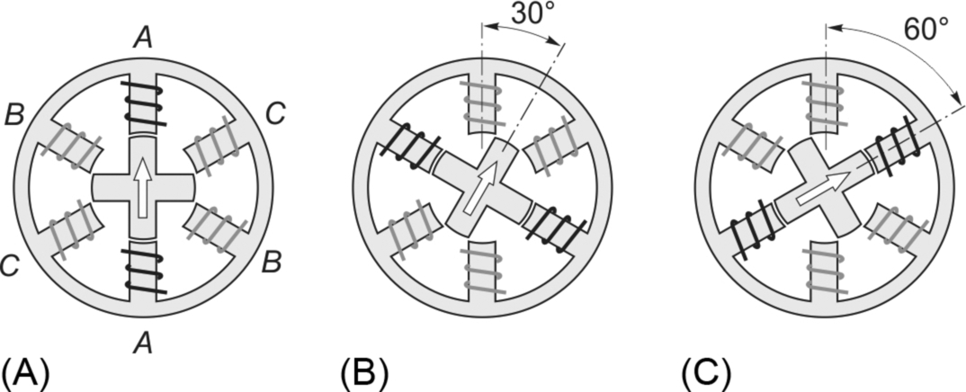
A simplified diagram of a 30°/step VR stepping motor is shown in Fig. 10.5. The stator is made from a stack of steel laminations, and has six equally-spaced projecting poles, or teeth, each carrying a separate coil. The rotor, which may be solid or laminated, has four projecting teeth, of the same width as the stator teeth. There is a very small air gap—typically between 0.02 mm and 0.2 mm—between rotor and stator teeth. When no current is flowing in any of the stator coils, the rotor will therefore be completely free to rotate.
Diametrically opposite pairs of stator coils are connected in series, such that when one of them acts as a North pole, the other acts as a South pole. There are thus three independent stator circuits, or phases, and each one can be supplied with direct current from the drive circuit (not shown in Fig. 10.5).
When phase A is energised (as indicated by the thick lines in Fig. 10.5A), a magnetic field with its axis along the stator poles of phase A is created. The rotor is therefore attracted into a position where the pair of rotor poles distinguished by the marker arrow line up with the field, i.e. in line with the phase-A pole, as shown in Fig. 10.5A. When phase A is switched off, and phase B is switched on instead, the second pair of rotor poles will be pulled into alignment with the stator poles of phase B, the rotor moving through 30° clockwise to its new step position, as shown in Fig. 10.5B. A further clockwise step of 30° will occur when phase B is switched off and phase C is switched on. At this stage the original pair of rotor poles come into play again, but this time they are attracted to stator poles C, as shown in Fig. 10.5C. By repetitively switching-on the stator phases in the sequence ABCA, etc. the rotor will rotate clockwise in 30° steps, while if the sequence is ACBA, etc. it will rotate anticlockwise. This mode of operation is known as ‘1-phase-on’, and is the simplest way of making the motor step. Note that the polarity of the energising current is not significant: the motor will be aligned equally well regardless of the direction of current.
This example demonstrates an interesting difference between doubly-salient reluctance motors and the singly-salient types discussed in Chapter 9. In a singly-salient machine, the pole-number of the field produced by the stator is determined by the winding layout and is the same as the number of rotor saliences, and both rotate together in the same direction. In most doubly-salient types, however, the rotor rotates in the opposite direction from the progression of the stator excitation: in Fig. 10.5 for example, the stator (2-pole) excitation axis rotates 60° anticlockwise each step, while the (4-pole) rotor turns 30° clockwise each step.
10.3.2 Hybrid motor
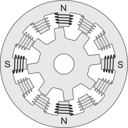
A cross-sectional view of a typical 1.8° hybrid motor is shown in Fig. 10.6. The stator has 8 main poles, each with 5 teeth, and each main pole carries a simple coil. The rotor has two steel end-caps, each with 50 teeth, and separated by a permanent magnet.
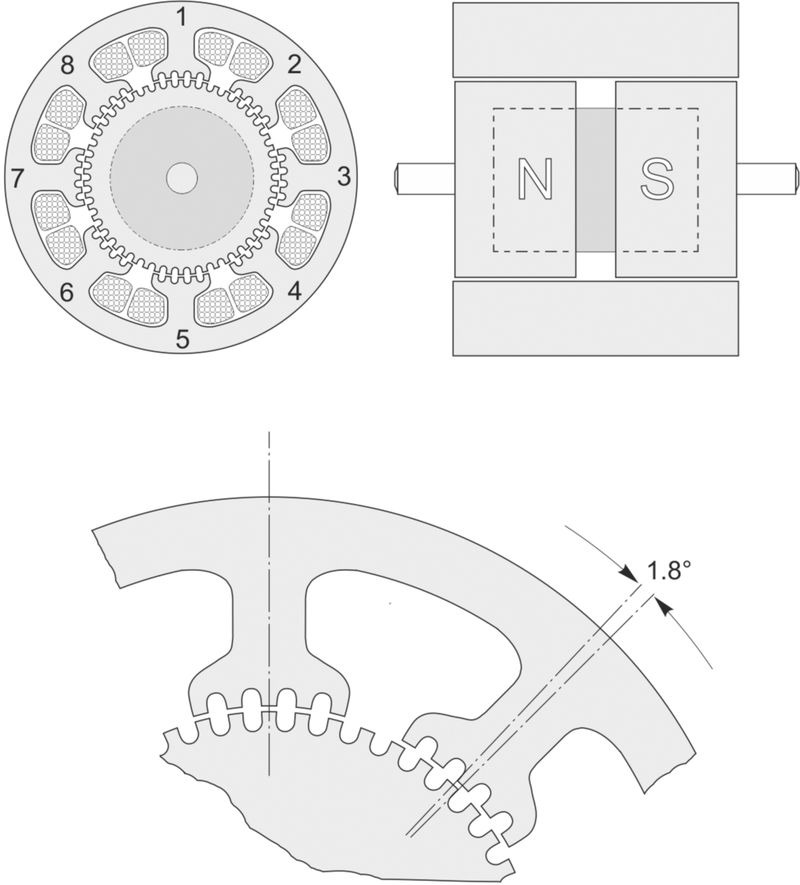
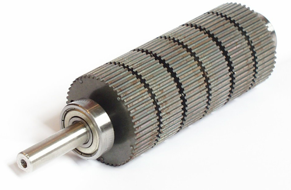
The rotor teeth have the same pitch as the teeth on the stator poles, and are offset so that the centreline of a tooth at one end-cap coincides with a slot at the other end-cap. The permanent-magnet is axially magnetised, so that one set of rotor teeth is given a North polarity, and the other a South polarity. Extra torque is obtained by adding more stacks, and stretching the stator, as shown in Fig. 10.7.
When no current is flowing in the windings, the only source of magnetic flux across the air-gap is the permanent magnet. The magnet flux crosses the air-gap from the N end-cap into the stator poles, flows axially along the body of the stator, and returns to the magnet by crossing the air-gap to the S end-cap. If there were no offset between the two sets of rotor teeth, there would be a strong periodic alignment torque when the rotor was turned, and every time a set of stator teeth was in line with the rotor teeth we would obtain a stable equilibrium position. However there is an offset, and this causes the alignment torque due to the magnet to be almost eliminated. In practice a small ‘detent’ torque remains, and this can be felt if the shaft is turned when the motor is de-energised: the motor tends to be held in its step positions by the detent torque. This is sometimes very useful: for example it is usually enough to hold the rotor stationary when the power is switched-off, so the motor can be left without fear of it being accidentally nudged into to a new position.
The 8 coils are connected to form two phase-windings. The coils on poles 1, 3, 5, and 7 form phase A, while those on 2, 4, 6, and 8 form phase B. When phase A carries positive current stator poles 1 and 5 are magnetised as South, and poles 3 and 7 become North. The teeth on the North end of the rotor are attracted to poles 1 and 5 while the offset teeth at the South end of the rotor are attracted into line with the teeth on poles 3 and 7. To make the rotor step, phase A is switched off, and phase B is energised with either positive current or negative current, depending on the sense of rotation required. This will cause the rotor to move by one quarter of a tooth pitch (1.8°) to a new equilibrium (step) position.
The motor is continuously stepped by energising the phases in the sequence + A, − B, − A, + B, + A (clockwise) or + A, + B, − A, − B, + A (anticlockwise). It will be clear from this that a bipolar supply is needed (i.e. one which can furnish + ve or − ve current). When the motor is operated in this way it is referred to as ‘2-phase, with bipolar supply’.
If a bipolar supply is not available, the same pattern of pole energisation may be achieved in a different way, as long as the motor windings consist of two identical (‘bifilar wound’) coils. To magnetise pole 1 North, a positive current is fed into one set of phase-A coils. But to magnetise pole 1 South, the same positive current is fed into the other set of phase-A coils, which have the opposite winding sense. In total, there are then four separate windings, and when the motor is operated in this way it is referred to as ‘4-phase, with unipolar supply’. Since each winding only occupies half of the space, the m.m.f. of each winding is only half of that of the full coil, so the thermally-rated output is clearly reduced as compared with bipolar operation (for which the whole winding is used).
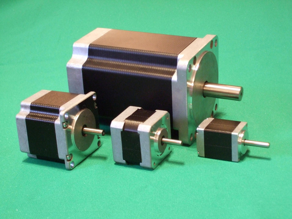
The 200 step/rev hybrid is the most widely-used general-purpose stepper, and is available in a range of sizes, as shown in Fig. 10.8.
We round-off this section on hybrid motors with a comment on identifying windings, and a warning. If the motor details are not known, it is usually possible to identify bifilar windings by measuring the resistance from the common to the two ends. If the motor is intended for unipolar drive only, one end of each winding may be commoned inside the casing; for example a 4-phase unipolar motor may have only five leads, one for each phase and one common. Wires are also usually colour-coded to indicate the location of the windings; for example a bifilar winding on one set of poles will have one end red, the other end red and white, and the common white. Finally, it is not advisable to remove the rotor of a hybrid motor because they are magnetised in-situ: removal typically causes a 5–10% reduction in magnet flux, with a corresponding reduction in static torque at rated current.
10.3.3 Summary
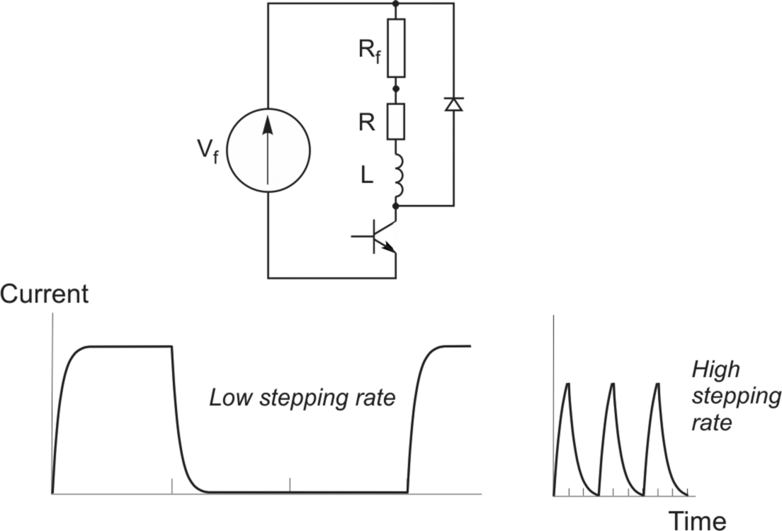
The construction of stepping motors is simple and robust, the only moving part being the rotor, which has no windings, commutator or brushes. The rotor is held at its step position solely by the action of the magnetic flux between stator and rotor. The step angle is a property of the tooth geometry and the arrangement of the stator windings, and accurate punching and assembly of the stator and rotor laminations is therefore necessary to ensure that adjacent step positions are exactly equally spaced. Any errors due to inaccurate punching will be non-cumulative, however.
The step angle is obtained from the expression
The VR motor in Fig. 10.5 has 4 rotor teeth, 3 stator phase-windings, and the step angle is therefore 30°, as already shown. It should also be clear from the equation why small angle motors always have to have a large number of rotor teeth: the 200 step/rev hybrid type (see Fig. 10.6) has a 50-tooth rotor, 4-phase stator, and hence a step angle of 1.8° (= 360°/(50 × 4).
The magnitude of the aligning torque clearly depends on the magnitude of the current in the phase-winding. However, the equilibrium positions itself does not depend on the magnitude of the current, because it is simply the position where the rotor and stator teeth are in line. This property underlines the digital nature of the stepping motor.
10.4 Motor characteristics
10.4.1 Static torque–displacement curves
From the previous discussion, it should be clear that the shape of the torque–displacement curve, and the peak static torque, will depend on the internal electromagnetic design of the rotor. In particular the shapes of the rotor and stator teeth, and the disposition of the stator windings (and permanent magnet(s)) all have to be optimised to obtain the maximum static torque.
We now turn to a typical static torque–displacement curve, and look at how it determines motor behaviour. Several aspects will be discussed, including the explanation of basic stepping (which has already been looked at in a qualitative way); the influence of load torque on step position accuracy; the effect of the amplitude of the winding current; and half-step and mini-stepping operation. For the sake of simplicity, the discussion will be based on the 30°/step 3-phase VR motor introduced earlier, but the conclusions reached apply to any stepping motor.
Typical static torque–displacement curves for a 3-phase 30°/step VR motor are shown in Fig. 10.9. These show the torque that has to be applied to move the rotor away from its aligned position. Because of the rotor/stator symmetry, the magnitude of the restoring torque when the rotor is displaced by a given angle in one direction is the same as the magnitude of the restoring torque when it is displaced by the same angle in the other direction, but of opposite sign.

There are 3 curves in Fig. 10.9, one for each of the three phases, and for each curve we assume that the relevant phase winding carries its full (rated) current. If the current is less than rated, the peak torque will be reduced, and the shape of the curve is likely to be somewhat different. The convention used in Fig. 10.9 is that a clockwise displacement of the rotor corresponds to a movement to the right, while a positive torque tends to move the rotor anticlockwise.
When only one phase, say A, is energised, the other two phases exert no torque, so their curves can be ignored and we can focus attention on the solid line in Fig. 10.9. Stable equilibrium positions (for phase A excited) exist at θ = 0°, 90°, 180° and 270°. They are stable (step) positions because any attempt to move the rotor away from them is resisted by a counteracting or restoring torque. These points correspond to positions where successive rotor poles (which are 90° apart) are aligned with the stator poles of phase A, as shown in Fig. 10.5A. There are also four unstable equilibrium positions, (at θ = 45°, 135°, 225° and 315°) at which the torque is also zero. These correspond to rotor positions where the stator poles are mid-way between two rotor poles, and they are unstable because if the rotor is deflected slightly in either direction, it will be accelerated in the same direction until it reaches the next stable position. If the rotor is free to turn, it will therefore always settle in one of the four stable positions.
10.4.2 Single-stepping
If we assume that phase A is energised, and the rotor is at rest in the position θ = 0° (Fig. 10.9) we know that if we want to step in a clockwise direction, the phases must be energised in the sequence ABCA, etc., so we can now imagine that phase A is switched off, and phase B is energised instead. We will also assume that the decay of current in phase A and the build-up in phase B take place very rapidly, before the rotor moves significantly.
The rotor will find itself at θ = 0°, but it will now experience a clockwise torque (see Fig. 10.9) produced by phase B. The rotor will therefore accelerate clockwise, and will continue to experience clockwise torque, until it has turned through 30°. The rotor will be accelerating all the time, and it will therefore overshoot the 30° position, which is of course its target (step) position for phase B. As soon as it overshoots, however, the torque reverses, and the rotor experiences a braking torque, which brings it to rest before accelerating it back towards the 30° position. If there was no friction or other cause of damping, the rotor would continue to oscillate; but in practice it comes to rest at its new position quite quickly in much the same way as a damped second-order system. The next 30° step is achieved in the same way, by switching-off the current in phase B, and switching-on phase C.
In the discussion above, we have recognised that the rotor is acted on sequentially by each of the three separate torque curves shown in Fig. 10.9. Alternatively, since the three curves have the same shape, we can think of the rotor being influenced by a single torque curve which ‘jumps’ by one step (30° in this case) each time the current is switched from one phase to the next. This is often the most convenient way of visualising what is happening in the motor.
10.4.3 Step position error, and holding torque
In the previous discussion the load torque was assumed to be zero, and the rotor was therefore able to come to rest with its poles exactly in line with the excited stator poles. When load torque is present, however, the rotor will not be able to pull fully into alignment, and a ‘step position error' will be unavoidable.
The origin and extent of the step position error can be appreciated with the aid of the typical torque–displacement curve shown in Fig. 10.10. The true step position is at the origin in the figure, and this is where the rotor would come to rest in the absence of load torque. If we imagine the rotor is initially at this position, and then consider that a clockwise load (TL) is applied, the rotor will move clockwise, and as it does so it will develop progressively more anticlockwise torque. The equilibrium position will be reached when the motor torque is equal and opposite to the load torque, i.e. at point A in Fig. 10.10. The corresponding angular displacement from the step position (θe in Fig. 10.10) is the step position error.

The existence of a step position error is one of the drawbacks of the stepping motor. The motor designer attempts to combat the problem by aiming to produce a steep torque–angle curve around the step position, and the user has to be aware of the problem and choose a motor with a sufficiently steep curve to keep the error within acceptable limits. In some cases this may mean selecting a motor with a higher peak torque than would otherwise be necessary, simply to obtain a steep enough torque curve around the step position.
As long as the load torque is less than Tmax (see Fig. 10.10), a stable rest position is obtained, but if the load torque exceeds Tmax, the rotor will be unable to hold its step position. Tmax is therefore known as the ‘holding’ torque. The value of the holding torque immediately conveys an idea of the overall capability of any motor, and it is—after step angle—the most important single parameter which is looked for in selecting a motor. Often, the adjective ‘holding’ is dropped altogether: for example ‘a 1 Nm motor' is understood to be one with a peak static torque (holding torque) of 1 Nm.
10.4.4 Half stepping
We have already seen how to step the motor in 30° increments by energising the phases one at a time in the sequence ABCA, etc. Although this ‘1-phase-on’ mode is the simplest and most widely used, there are two other modes which are also frequently employed. These are referred to as the ‘2-phase-on’ mode and the ‘half-stepping’ mode. The 2-phase-on can provide greater holding torque and a much better damped single-step response than the 1-phase-on mode; and the half stepping mode permits the effective step angle to be halved—thereby doubling the resolution - and produces a smoother shaft rotation.
In the 2-phase-on mode, two phases are excited simultaneously. When phases A and B are energised, for example, the rotor experiences torques from both phases, and comes to rest at a point midway between the two adjacent full step positions. If the phases are switched in the sequence AB, BC, CA, AB, etc., the motor will take full (30°) steps, as in the 1-phase-on mode, but its equilibrium positions will be interleaved between the full-step positions.
To obtain ‘half-stepping’ the phases are excited in the sequence A, AB, B, BC, etc., i.e. alternately in the 1-phase-on and 2-phase-on modes. This is sometimes known as ‘wave’ excitation, and it causes the rotor to advance in steps of 15°, or half the full step angle. As might be expected, continuous half-stepping usually produces a smoother shaft rotation than full-stepping, and it also doubles the resolution.
We can see what the static torque curve looks like when two phases are excited by superposition of the individual phase curves. An example is shown in Fig. 10.11, from which it can be seen that for this machine, the holding torque (i.e. the peak static torque) is higher with two phases excited than with only one excited. The stable equilibrium (half-step) position is at 15°, as expected. The price to be paid for the increased holding torque is the increased power dissipation in the windings, which is doubled as compared with the 1-phase-on mode. The holding torque increases by a factor less than two, so the torque per watt (which is a useful figure of merit) is reduced.

A word of caution is needed in regard to the addition of the two separate 1-phase-on torque curves to obtain the 2-phase-on curve. Strictly, such a procedure is only valid where the two phases are magnetically independent, or the common parts of the magnetic circuits are unsaturated. This is not the case in most motors, in which the phases share a common magnetic circuit which operates under highly saturated conditions. Direct addition of the 1-phase-on curves cannot therefore be expected to give an accurate result for the 2-phase-on curve, but it is easy to do, and provides a reasonable estimate.
Apart from the higher holding torque in the 2-phase-on mode, there is another important difference which distinguishes the static behaviour from that of the 1-phase-on mode. In the 1-phase-on mode, the equilibrium or step positions are determined solely by the geometry of the rotor and stator: they are the positions where the rotor and stator are in line. In the 2-phase-on mode, however, the rotor is intended to come to rest at points where the rotor poles are lined-up midway between the stator poles. This position is not sharply defined by the ‘edges’ of opposing poles, as in the 1-phase-on case; and the rest position will only be exactly midway if (a) there is exact geometrical symmetry and, more importantly (b) the two currents are identical. If one of the phase currents is larger than the other, the rotor will come to rest closer to the phase with the higher current, instead of half-way between the two. The need to balance the currents to obtain precise half stepping is clearly a drawback to this scheme. Paradoxically, however, the properties of the machine with unequal phase currents can sometimes be turned to good effect, as we now see.
10.4.5 Step division—Mini-stepping
There are some applications where very fine resolution is called for, and a motor with a very small step angle—perhaps only a fraction of a degree—is required. We have already seen that the step angle can only be made small by increasing the number of rotor teeth and/or the number of phases, but in practice it is inconvenient to have more than four or five phases, and it is difficult to manufacture rotors with more than 50–100 teeth. This means it is rare for motors to have step angles below about 1°. When a smaller step angle is required a technique known as mini-stepping (or step division) is used.
Mini-stepping is a technique based on 2-phase-on operation which provides for the sub-division of each full motor step into a number of ‘substeps’ of equal size. In contrast with half-stepping, where the two currents have to be kept equal, the currents are deliberately made unequal. By correctly choosing and controlling the relative amplitudes of the currents, the rotor equilibrium position can be made to lie anywhere between the step positions for each of the two separate phases.
Closed-loop current control is needed to prevent the current from changing as a result of temperature changes in the windings, or variations in the supply voltage; and if it is necessary to ensure that the holding torque stays constant for each mini-step both currents must be changed according to a prescribed algorithm. Despite the difficulties referred to above, mini-stepping is used extensively, especially in photographic and printing applications where a high resolution is needed. Schemes involving between 3 and 10 mini-steps for a 1.8° step motor are numerous, and there are instances where over 100 mini-steps (20,000 mini-steps/rev) have been achieved.
So far, we have concentrated on those aspects of behaviour which depend only on the motor itself, i.e. the static performance. The shape of the static torque curve, the holding torque, and the slope of the torque curve about the step position have all been shown to be important pointers to the way the motor can be expected to perform. All of these characteristics depend on the current(s) in the windings, however, and when the motor is running the instantaneous currents will depend on the type of drive circuit employed.
10.5 Steady-state characteristics—Ideal (constant-current) drive
In this section we will look first at how the motor would perform if it were supplied by an ideal drive circuit, which turns out to be one that is capable of supplying rectangular pulses of current to each winding when required, and regardless of the stepping rate. Because of the inductance of the windings, no real drive circuit will be able to achieve this, but the most sophisticated (and expensive) ones achieve near-ideal operation up to very high stepping rates.
10.5.1 Requirements of drive
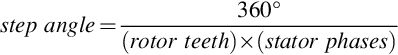
The basic function of the complete drive is to convert the step command input signals into appropriate patterns of currents in the motor windings. This is achieved in two distinct stages, as shown in Fig. 10.12, which relates to a 3-phase motor.
The ‘translator' stage converts the incoming train of step command pulses into a sequence of on/off commands to each of the three power stages. In the 1 phase-on mode, for example, the first step command pulse will be routed to turn on phase A, the second will turn on phase B, and so on. In a very simple drive, the translator will probably provide for only one mode of operation (e.g. 1-phase-on), but most commercial drives provide the option of 1-phase-on, 2-phase on and half-stepping. Single-chip I.C.’s with these 3 operating modes and with both 3-phase and 4-phase outputs are readily available.
The power stages (one per phase) supply the current to the windings. An enormous diversity of types are in use, ranging from simple ones with one switching transistor per phase, to elaborate chopper-type circuits with four transistors per phase, and some of these are discussed in Section 10.6. At this point however, it is helpful to list the functions required of the ‘ideal' power stage. These are firstly that when the translator calls for a phase to be energised, the full (rated) current should be established immediately; secondly, the current should be maintained constant (at its rated value) for the duration of the ‘on’ period; and finally, when the translator calls for the current to be turned off, it should be reduced to zero immediately.
The ideal current waveforms for continuous stepping with 1-phase-on operation are shown in the lower part of Fig. 10.12. The currents have a square profile because this leads to the optimum value of running torque from the motor. But because of the inductance of the windings, no real drive will achieve the ideal current wave-forms, though many drives come close to the ideal, even at quite high stepping rates. Drives which produce such rectangular current waveforms are (not surprisingly) called constant-current drives. We now look at the running torque produced by a motor when operated from an ideal constant current drive. This will act as a yardstick for assessing the performance of other drives, all of which will be seen to have inferior performance.
10.5.2 Pull-out torque under constant-current conditions
If the phase currents are taken to be ideal, i.e. they are switched on and off instantaneously, and remain at their full rated value during each ‘on’ period, we can picture the axis of the magnetic field to be advancing around the machine in a series of steps, the rotor being urged to follow it by the reluctance torque. If we assume that the inertia is high enough for fluctuations in rotor velocity to be very small, the rotor will be rotating at a constant rate which corresponds exactly to the stepping rate.
Now if we consider a situation where the position of the rotor axis is, on average, lagging behind the advancing field axis, it should be clear that, on average, the rotor will experience a driving torque. The more it lags behind, the higher will be the average forward torque acting on it, but only up to a point. We already know that if the rotor axis is displaced too far from the field axis, the torque will begin to diminish, and eventually reverse, so we conclude that although more torque will be developed by increasing the rotor lag angle, there will be a limit to how far this can be taken.
Turning now to a quantitative examination of the torque on the rotor, we will make use of the static torque–displacement curves discussed earlier, and look at what happens when the load on the shaft is varied, the stepping rate being kept constant. Clockwise rotation will be studied, so the phases will be energised in the sequence ABC. The instantaneous torque on the rotor can be arrived at by recognising (a) that the rotor speed is constant, and it covers one step angle (30°) between step command pulses, and (b) the rotor will be ‘acted on’ sequentially by each of the set of torque curves.
When the load torque is zero, the net torque developed by the rotor must be zero (apart from a very small torque required to overcome friction). This condition is shown in Fig. 10.13A. The instantaneous torque is shown by the thick line, and it is clear that each phase in turn exerts first a clockwise torque, then an anticlockwise torque while the rotor angle turns through 30°. The average torque is zero, the same as the load torque, because the average rotor lag angle is zero.

When the load torque on the shaft is increased, the immediate effect is to cause the rotor to fall back in relation to the field. This causes the clockwise torque to increase, and the anticlockwise torque to decrease. Equilibrium is reached when the lag angle has increased sufficiently for the motor torque to equal the load torque. The torque developed at an intermediate load condition like this is shown by the thick line in Fig. 10.13B. The highest average torque that can possibly be developed is shown by the thick line in Fig. 10.13C: if the load torque exceeds this value (which is known as the pull-out torque) the motor loses synchronism and stalls, and the vital one-to-one correspondences between pulses and steps is lost.
Since we have assumed an ideal constant-current drive, the pull-out torque will be independent of the stepping rate, and the pull-out torque–speed curve under ideal conditions is therefore as shown in Fig. 10.14. The shaded area represents the permissible operating region: at any particular speed (stepping rate) the load torque can have any value up to the pull-out torque, and the motor will continue to run at the same speed. But if the load torque exceeds the pull-out torque, the motor will suddenly pull out of synchronism and stall.

As mentioned earlier, no real drive will be able to provide the ideal current waveforms, so we now turn to look briefly at the types of drives in common use, and at their pull-out torque–speed characteristics.
10.6 Drive circuits and pull-out torque–speed curves
Users often find difficulty in coming to terms with the fact that the running performance of a stepping motor depends so heavily on the type of drive circuit being used. It is therefore important to emphasise that in order to meet a specification, it will always be necessary to consider the motor and drive together, as a package.
There are three commonly-used types of drive. All use transistors which are operated as switches, i.e. they are either turned fully on, or they are cut-off. A brief description of each is given below, and the pros and cons of each type are indicated. In order to simplify the discussion, we will consider one phase of a 3-phase VR motor and assume that it can be represented by a simple series R-L circuit in which R and L are the resistance and self-inductance of the winding respectively. (In practice the inductance will vary with rotor position, giving rise to motional e.m.f. in the windings, which, as we have seen previously in this book, is an inescapable manifestation of an electromechanical energy-conversion process. If we needed to analyse stepping motor behaviour fully we would have to include the motional e.m.f. terms. Fortunately, we can gain a pretty good appreciation of how the motor behaves if we model each winding simply in terms of its resistance and self-inductance.)
10.6.1 Constant voltage drive
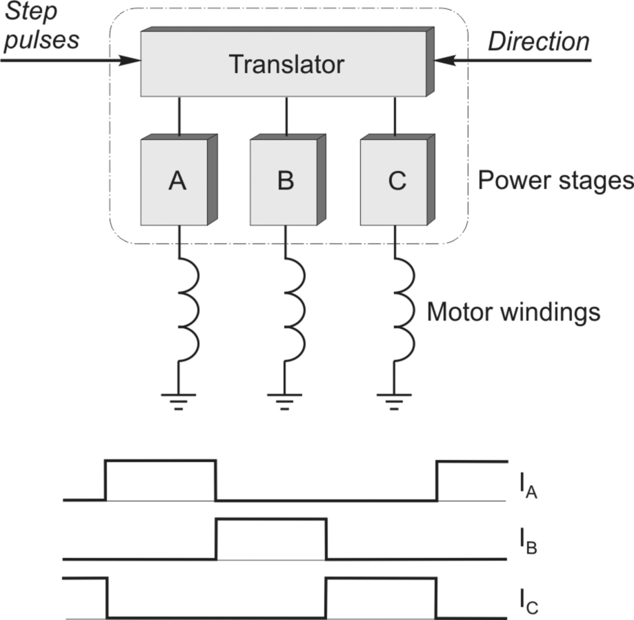
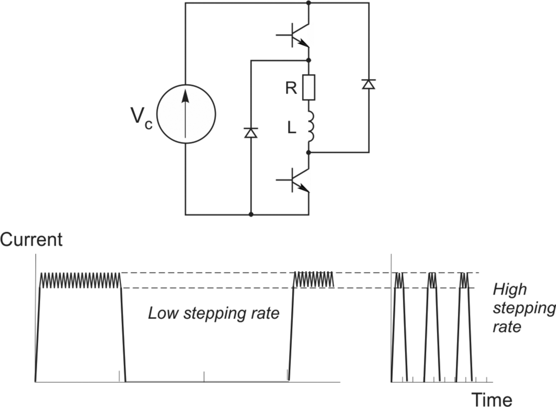
This is the simplest possible drive: the circuit for one of the three phases is shown in the upper part of Fig. 10.15, and the current waveforms at low and high stepping rates are shown in the lower part of the figure. The d.c. voltage V is chosen so that when the switching device (usually a MOSFET although a BJT is shown) turns on, the steady current is the rated current as specified by the motor manufacturer.
The current waveforms display the familiar rising exponential shape that characterises a first-order system: the time-constant is L/R, the current reaching its steady state after several time-constants. When the transistor switches off, the stored energy in the inductance cannot instantaneously reduce to zero, so although the current through the transistor suddenly becomes zero, the current in the winding is diverted into the closed path formed by the winding and the freewheel diode, and it then decays exponentially to zero, again with time-constant L/R: in this period the stored energy in the magnetic field is dissipated as heat in the resistance of the winding and diode.
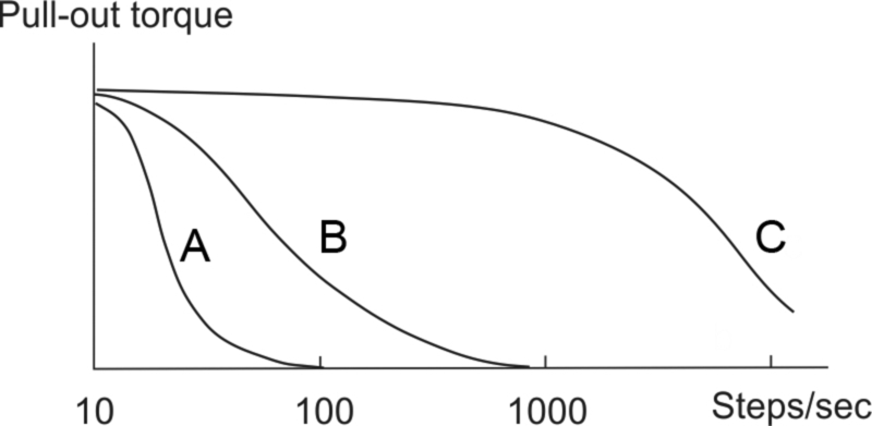
At low stepping rates (low speed), the drive provides a reasonably good approximation to the ideal rectangular current waveform. (We are considering a 3-phase motor, so ideally one phase should be on for one step pulse and off for the next two, as in Fig. 10.12.) But at higher frequencies (right-hand waveform in Fig. 10.15), where the ‘on’ period is short compared with the winding time-constant, the current waveform degenerates, and is nothing like the ideal rectangular shape. In particular the current never gets anywhere near its full value during the on pulse, so the torque over this period is reduced; and even worse, a substantial current persists when the phase is supposed to be off, so during this period the phase will contribute a negative torque to the rotor. Not surprisingly all this results in a very rapid fall-off of pull-out torque with speed, as shown later in Fig. 10.18A.
Curve (A) in Fig. 10.18 should be compared with the pull-out torque under ideal constant-current conditions shown in Fig. 10.14 in order to appreciate the severely limited performance of the simple constant-voltage drive.
10.6.2 Current-forced drive
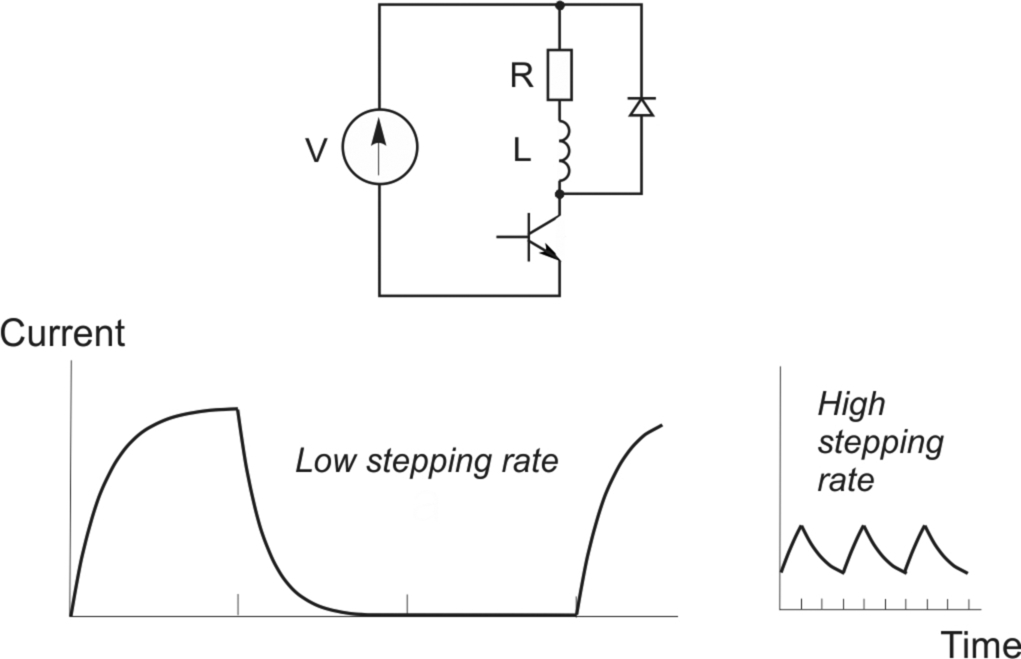
The initial rate of rise of current in a series R-L circuit is directly proportional to the applied voltage, so in order to establish the current more quickly at switch-on, a higher supply voltage (Vf) is needed. But if we simply increased the voltage, the steady-state current (Vf/R) would exceed the rated current and the winding would overheat.
To prevent the current from exceeding the rated value, an additional ‘forcing’ resistor has to be added in series with the winding. The value of this resistance (Rf) must be chosen so that (Vf/(R + Rf) = I,where I is the rated current. This is shown in the upper part of Fig. 10.16, together with the current waveforms at low and high stepping rates. Because the rates of rise and fall of current are higher, the current waveforms approximate more closely to the ideal rectangular shape, especially at low stepping rates, though at higher rates they are still far from ideal, as shown in Fig. 10.16. The low-frequency pull-out torque is therefore maintained to a higher stepping rate, as shown in Fig. 10.18B. Values of Rf from 2 to 10 times the motor resistance (R) are common. Broadly speaking, if Rf = 10R, for example, a given pull-out torque will be available at ten-times the stepping rate, compared with an unforced constant-voltage drive.
Manufacturers sometimes call this type of drive an ‘R/L' drive, or an ‘L/R' drive, or even simply a ‘Resistor Drive’. Sets of pull-out torque speed curves in catalogues may be labelled with values R/L (or L/R) = 5, 10, etc. This means that the curves apply to drives where the forcing resistor is five (or ten) times the winding resistance, the implication being that the drive voltage has also been adjusted to keep the static current at its rated value. Obviously, it follows that the higher Rf is made, the higher the power rating of the supply; and it is the higher power rating which is the principal reason for the improved torque–speed performance.
The major disadvantage of this drive is its inefficiency, and the consequent need for a high power-supply rating. Large amounts of heat are dissipated in the forcing resistors, especially when the motor is at rest and the phase-current is continuous, and disposing of the heat can lead to awkward problems in the siting of the forcing resistors. These drives are therefore only used at the low-power end of the scale.
It was mentioned earlier that the influence of the motional e.m.f. in the winding would be ignored. In practice, however, the motional e.m.f. always has a pronounced influence on the current, especially at high stepping rates, so it must be borne in mind that the waveforms shown in Figs. 10.15 and 10.16 are only approximate. Not surprisingly, it turns out that the motional e.m.f. tends to make the current waveforms worse (and the torque less) than the discussion above suggests. Ideally therefore, we need a drive which will keep the current constant throughout the on period, regardless of the motional e.m.f. The closed-loop chopper-type drive (below) provides the closest approximation to this, and it avoids the waste of power which is a feature of R/L drives, so this type is now the most widely used.
10.6.3 Constant current (chopper) drive
The basic circuit for one phase of a VR motor is shown in the upper part of Fig. 10.17, with the current wave-forms shown below. A high-voltage power supply is used in order to obtain very rapid changes in current when the phase is switched on or off.
The lower transistor is turned on for the whole period during which current is required. The upper transistor turns on whenever the actual current falls below the lower threshold of the hysteresis band (shown dotted in Fig. 10.17) and it turns off when the current exceeds the upper threshold. The chopping action leads to a current waveform which is a good approximation to the ideal (see Fig. 10.12). At the end of the on period both transistors switch off and the current freewheels through both diodes and back to the supply. During this period the stored energy in the inductance is returned to the supply, and because the winding terminal voltage is then −Vc, the current decays as rapidly as it built up.
Because the current-control system is a closed-loop one, distortion of the current waveform by the motional e.m.f. is minimised, and this means that the ideal (constant-current) torque–speed curve is closely followed up to high stepping rates. Eventually, however, the ‘on’ period reduces to the point where it is less than the current rise time, and the full current is never reached. Chopping action then ceases, the drive reverts essentially to a constant-voltage one, and the torque falls rapidly as the stepping rate is raised even higher, as in Fig. 10.18C. There is no doubt of the overall superiority of the chopper-type drive, and it is now the standard drive. Single-chip chopper modules can be bought for small (say 1–2 A) motors: complete plug-in chopper cards rated up to 10 A or more are available for larger motors; and increasingly, motors may have the drive integrated with the motor housing.
The discussion in this section relates to a VR motor, for which unipolar current pulses are sufficient. If we have a hybrid or other permanent-magnet motor we will need a bipolar current source (i.e. one that can provide positive or negative current), and for this we will find that each phase is supplied from a 4-transistor H-bridge, as discussed in Chapter 2. A typical bipolar drive for a hybrid motor is shown in Fig. 10.19.

10.6.4 Resonances and instability
In practice, measured torque–speed curves frequently display severe dips at or around certain stepping rates: a typical measured characteristic for a hybrid motor with a voltage-forced drive is shown as (a) in Fig. 10.20. Manufacturers are not keen to stress this feature, so it is important for the user to be aware of the potential difficulty.

The magnitude and location of the torque dips depend in a complex way on the characteristics of the motor, the drive, the operating mode and the load. We will not go into detail here, apart from mentioning the underlying causes and remedies.
There are two distinct mechanisms which cause the dips. The first is a straightforward ‘resonance-type’ problem which manifests itself at low stepping rates, and originates from the oscillatory nature of the single-step response. Whenever the stepping rate coincides with the natural frequency of rotor oscillations, the oscillations can be enhanced, and this in turn makes it more likely that the rotor will fail to keep in step with the advancing field.
The second phenomenon occurs because at certain stepping rates it is possible for the complete motor/drive system to exhibit positive feedback, and become unstable. This instability usually occurs at relatively high stepping rates, well above the ‘resonance’ regions discussed above. The resulting dips in the torque–speed curve are extremely sensitive to the degree of viscous damping present (mainly in the bearings), and it is not uncommon to find that a severe dip which is apparent on a warm day (such as that shown at around 1000 steps/s in Fig. 10.20) will disappear on a cold day.
The dips are most pronounced during steady-state operation, and it may be that their presence is not serious provided that continuous operation at the relevant speeds is not required. In this case, it is often possible to accelerate through the dips without adverse effect. Various special drive techniques exist for eliminating resonances by smoothing out the step-wise nature of the stator field, or by modulating the supply frequency to damp out the instability, but the simplest remedy in open-loop operation is to fit a damper to the motor shaft. Dampers of the Lanchester type or of the viscously-coupled inertia (VCID) type are used. These consist of a lightweight housing which is fixed rigidly to the motor shaft, and an inertia which can rotate relative to the housing. The inertia and the housing are separated either by a viscous fluid (VCID type) or by a friction disc (Lanchester type). Whenever the motor speed is changing, the assembly exerts a damping torque, but once the motor speed is steady, there is no drag torque from the damper. By selecting the appropriate damper, the dips in the torque speed curve can be eliminated, as shown in Fig. 10.20(b). Dampers are also often essential to damp the single-step response, particularly with VR motors, many of which have a highly oscillatory step response. Their only real drawback is that they increase the effective inertia of the system, and thus reduces the maximum acceleration.
10.7 Transient performance
10.7.1 Step response
It was pointed out earlier that the single-step response is similar to that of a damped second-order system. We can easily estimate the natural frequency ωn in rad/s from the equation
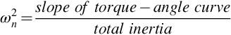
Knowing ωn, we can judge what the oscillatory part of the response will look like, by assuming the system is undamped. To refine the estimate, and to obtain the settling time, however, we need to estimate the damping ratio, which is much more difficult to determine as it depends on the type of drive circuit and mode of operation as well as on the mechanical friction. In VR motors the damping ratio can be as low as 0.1, but in hybrid types it is typically 0.3–0.4. These values are too low for many applications where rapid settling is called for.
Two remedies are available, the simplest being to fit a mechanical damper of the type mentioned above. Alternatively, a special sequence of timed command pulses can be used to brake the rotor so that it reaches its new step position with zero velocity and does not overshoot. This procedure is variously referred to as ‘electronic damping’, ‘electronic braking’ or ‘back phasing’. It involves re-energising the previous phase for a precise period before the rotor has reached the next step position, in order to exert just the right degree of braking. It can only be used successfully when the load torque and inertia are predictable and not subject to change. Because it is an open-loop scheme it is extremely sensitive to apparently minor changes such as day-to-day variation in friction, which can make it unworkable in many instances.
10.7.2 Starting from rest
The rate at which the motor can be started from rest without losing steps is known as the ‘starting’ or ‘pull-in’ rate. The starting rate for a given motor depends on the type of drive, and the parameters of the load. This is entirely as expected since the starting rate is a measure of the motor's ability to accelerate its rotor and load and pull into synchronism with the field. The starting rate thus reduces if either the load torque, or the load inertia are increased. Typical pull-in torque–speed curves, for various inertias, are shown in Fig. 10.21. The pull-out torque speed curve is also shown, and it can be seen that for a given load torque, the maximum steady (slewing) speed at which the motor can run is much higher than the corresponding starting rate. (Note that only one pull-out torque is usually shown, and is taken to apply for all inertia values. This is because the inertia is not significant when the speed is constant.)

It will normally be necessary to consult the manufacturer's data to obtain the pull-in rate, which will apply only to a particular drive. However, a rough assessment is easily made: we simply assume that the motor is producing its pull-out torque, and calculate the acceleration that this would produce, making due allowance for the load torque and inertia. If, with the acceleration as calculated, the motor is able to reach the steady speed in one step or less, it will be able to pull in; if not, a lower pull-in rate is indicated.
10.7.3 Optimum acceleration and closed-loop control
There are some applications where the maximum possible accelerations and decelerations are demanded, in order to minimise point-to-point times. If the load parameters are stable and well-defined, an open-loop approach is feasible, and this is discussed first. Where the load is unpredictable, however, a closed-loop strategy is essential, and this is dealt with later.
To achieve maximum possible acceleration calls for every step command pulse to be delivered at precisely optimised intervals during the acceleration period. For maximum torque, each phase must be on whenever it can produce positive torque, and off when its torque would be negative. Since the torque depends on the rotor position, the optimum switching times have to be calculated from a full dynamic analysis. This can usually be accomplished by making use of the static torque–angle curves (provided appropriate allowance is made for the rise and fall times of the stator currents), together with the torque–speed characteristic and inertia of the load. A series of computations is required to predict the rotor angle-time relationship, from which the switchover points from one phase to the next are deduced. The train of accelerating pulses is then pre-programmed into the controller, for subsequent feeding to the drive in an open-loop fashion. It is obvious that this approach is only practicable if the load parameters do not vary, since any change will invalidate the computed optimum stepping intervals.
When the load is unpredictable, a much more satisfactory arrangement is obtained by employing a closed-loop scheme, using position feedback from a shaft-mounted encoder. The feedback signals indicate the instantaneous position of the rotor, and are used to ensure that the phase-windings are switched at precisely the right rotor position for maximising the developed torque. Motion is initiated by a single command pulse, and subsequent step-command pulses are effectively self-generated by the encoder. The motor continues to accelerate until its load torque equals the load torque, and then runs at this (maximum) speed until the deceleration sequence is initiated. During all this time, the step counter continues to record the number of steps taken. This approach is essentially the same as we discussed in relation to self synchronous motors in Chapter 9.
Closed-loop operation ensures that the optimum acceleration is achieved, but at the expense of more complex control circuitry, and the need to fit a shaft encoder. Relatively cheap encoders are however now available for direct fitting to some ranges of motors, and single chip microcontrollers are available which provide all the necessary facilities for closed-loop control.
An appealing approach aimed at eliminating an encoder is to detect the position of the rotor by on-line analysis of the signals (principally the rates of change of currents) in the motor windings themselves: in other words, to use the motor as its own encoder. A variety of approaches have been tried, including the addition of high-frequency alternating voltages superimposed on the excited phase, so that as the rotor moves the variation of inductance results in a modulation of the alternating current component. Some success has been achieved with particular motors, but the approach has not achieved widespread commercial exploitation, perhaps because of competition from the PM synchronous drives discussed in Chapter 9.
To return finally to encoders, we should note that they are also used in open-loop schemes when an absolute check on the number of steps taken is required. In this context the encoder simply provides a tally of the total steps taken, and normally plays no part in the generation of the step pulses. At some stage, however, the actual number of steps taken will be compared with the number of step command pulses issued by the controller. When a disparity is detected, indicating a loss (or gain of steps), the appropriate additional forward or backward pulses can be added.
10.8 Switched reluctance motor drives
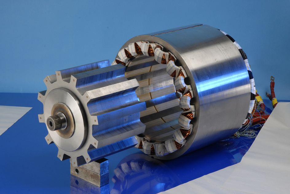
The switched reluctance drive was developed in the 1980s with the promise of offering advantages in terms of efficiency, power per unit weight and volume, robustness and operational flexibility compared with the then dominant induction motor. Its market position has been compromised by the rise of PM motor technologies and improved control strategies for induction motors. Nevertheless, the switched reluctance motor has been applied to a range of applications which can benefit from its performance characteristics, notably offering very high torque at standstill and very low speed. The motor (Fig. 10.22) and its associated power-electronic drive must be designed as an integrated package, and optimised for a particular specification, e.g. for maximum overall efficiency with a specific load, or maximum speed range, peak short-term torque or torque ripple (and associated acoustic noise).
10.8.1 Principle of operation
Like the stepping motor, the switched reluctance (SR) motor (Fig. 10.23) is ‘doubly-salient’, i.e. it has projecting poles on both rotor and stator. However, most SR motors are of much higher power than the largest stepper, and it turns out that in the higher power ranges (where the winding resistances become much less significant), the doubly-salient arrangement is very effective in terms of efficient electromagnetic energy conversion.
A cross section through a typical SR motor is shown in Fig. 10.23: this example has twelve stator poles and eight rotor poles, and represents a widely used arrangement, but other pole combinations are used to suit different applications. The stator carries coils on each pole, while the rotor, which is made from laminations in the usual way, has no windings or magnets.
In Fig. 10.23 the twelve coils are grouped to form three phases, which are independently energised from a three-phase converter.
The motor rotates by exciting the phases sequentially in the sequence A, B, C for anticlockwise rotation or A, C, B for clockwise rotation, the ‘nearest’ pair of rotor poles being pulled into alignment with the appropriate stator poles by reluctance torque action. In Fig. 10.23 the four coils forming phase A are shown in black, the polarities of the coil m.m.f.'s being indicated by the letters N and S on the back of core. Each time a new phase is excited the equilibrium position of the rotor advances by 15°, so after one complete cycle (i.e. each of the three phases has been excited once) the angle turned through is 45°. The machine therefore rotates once for eight fundamental cycles of supply to the stator windings, so in terms of the relationship between the fundamental supply frequency and the speed of rotation, the machine in Fig. 10.23 behaves as a 16-pole conventional machine.
The structure is clearly the same as the variable reluctance stepping motor discussed earlier in this chapter, but there are important design differences which reflect the different objectives (continuous rotation for the SR, stepwise progression for the stepper), but otherwise the mechanisms of torque production are identical. However whilst the stepper is designed first and foremost for open-loop operation, the SR motor is designed for self-synchronous operation, the phases being switched by signals derived from a shaft-mounted rotor position detector. In terms of performance, at all speeds below the base speed continuous operation at full torque is possible. Above the base speed, the flux can no longer be maintained at full amplitude and the available torque reduces with speed. The operating characteristics are thus very similar to those of the other most important controlled-speed drives.
10.8.2 Torque prediction and control
If the iron in the magnetic circuit is treated as ideal, analytical expressions can be derived to express the torque of a reluctance motor in terms of the rotor position and the current in the windings. In practice, however, this analysis is of little real use, not only because switched reluctance motors are designed to operate with high levels of magnetic saturation in parts of the magnetic circuit, but also because, except at low speeds, it is not easy to achieve specified current profiles.
The fact that high levels of saturation are involved makes the problem of predicting torque at the design stage challenging, but despite the highly non-linear relationships it is possible to compute the flux, current and torque as functions of rotor position, so that optimum control strategies can be devised to meet particular performance specifications. Unfortunately this complexity means that there is no simple equivalent circuit available to illuminate behaviour.
As we saw when we discussed the stepping motor, to maximise the average torque it would (in principle) be desirable to establish the full current in each phase instantaneously, and to remove it instantaneously at the end of each positive torque period. But, as illustrated in Fig. 10.15, this is not possible even with a small stepping motor, and certainly out of the question for switched reluctance motors (which have much higher inductance) except at low speeds where current-chopping (see Fig. 10.17) is employed. For most of the speed range, the best that can be done is to apply the full voltage available from the converter at the start of the ‘on’ period, and (using a circuit such as that shown in Fig. 10.17) apply full negative voltage at the end of the pulse by opening both of the switches.
Operation using full positive voltage at the beginning and full negative voltage at the end of the ‘on’ period is referred to as ‘single-pulse’ operation. For all but small motors (of less than say 1 kW) the phase resistance is negligible and consequently the magnitude of the phase flux-linkage is determined by the applied voltage and frequency, as we have seen many times previously with other types of motor.
The relationship between the flux-linkage (ψ) and the voltage is embodied in Faraday's law, i.e. ![]() , so with the rectangular voltage waveform of single-pulse operation the phase flux linkage waveforms have a very simple triangular shape, as in Fig. 10.24 which shows the waveforms for phase A of a 3-phase motor. (The waveforms for phases B are C are identical, but are not shown: they are displaced by one third and two thirds of a cycle, as indicated by the arrows.) The upper half of the diagram represents the situation at speed N, while the lower half corresponds to a speed of 2 N. As can be seen, at the higher speed (high frequency) the ‘on’ period halves, so the amplitude of the flux halves, leading to a reduction in available torque. The same limitation was seen in the case of the inverter-fed induction motor drive, the only difference being that the waveforms in that case were sinusoidal rather than triangular.
, so with the rectangular voltage waveform of single-pulse operation the phase flux linkage waveforms have a very simple triangular shape, as in Fig. 10.24 which shows the waveforms for phase A of a 3-phase motor. (The waveforms for phases B are C are identical, but are not shown: they are displaced by one third and two thirds of a cycle, as indicated by the arrows.) The upper half of the diagram represents the situation at speed N, while the lower half corresponds to a speed of 2 N. As can be seen, at the higher speed (high frequency) the ‘on’ period halves, so the amplitude of the flux halves, leading to a reduction in available torque. The same limitation was seen in the case of the inverter-fed induction motor drive, the only difference being that the waveforms in that case were sinusoidal rather than triangular.

It is important to note that these flux waveforms do not depend on the rotor position, but the corresponding current waveforms do because the m.m.f. needed for a given flux depends on the effective reluctance of the magnetic circuit, and this of course varies with the position of the rotor.
To get the most motoring torque for any given phase flux waveform, it is obvious that the rise and fall of the flux must be timed to coincide with the rotor position: ideally, the flux should only be present when it produces positive torque, and be zero whenever it would produce negative torque, but given the delay in build-up of the flux it may be better to switch on early so that the flux reaches a decent level at the point when it can produce the most torque, even if this does lead to some negative torque at the start and finish of the cycle.
The job of the torque control system is to switch each phase on and off at the optimum rotor position in relation to the torque being demanded at the time, and this is done by keeping track of the rotor position, possibly using a rotor position sensor.2 Just what angles constitute the optimum depends on what is to be optimised (e.g. average torque, overall efficiency), and this in turn is decided by reference to the data stored digitally in the controller ‘memory map’ that relates current, flux, rotor position and torque for the particular machine. Torque control is thus considerably less straightforward than in d.c. drives, where torque is directly proportional to armature current, or induction motor drives where torque is proportional to slip.
10.8.3 Power converter and overall drive characteristics
An important difference between the SR motor and all other self-synchronous motors is that its full torque capability can be achieved without having to provide for both positive and negative currents in the phases. This is because the torque does not depend on the direction of current in the phase winding. The advantage of such ‘unipolar' drives is that because each of the main switching devices is permanently connected in series with one of the motor windings (as in Fig. 10.17), there is no possibility of the ‘shoot-through’ fault (see Chapter 2) which necessitates the inclusion of ‘dead time’ in the switching strategies of the conventional inverter.
Overall closed-loop speed control is obtained in the conventional way with the speed error acting as a torque demand to the torque control system described above. However, if a position sensor is fitted the speed can be derived from the position signal.
In common with other self-synchronous drives, a wide range of operating characteristics are available. If the input converter is fully controlled, continuous regeneration and full 4-quadrant operation is possible, and the usual constant torque, constant power and series type characteristic is regarded as standard. Low speed torque can be uneven unless special measures are taken to profile the current pulses, but the particular merit of the SR drive is that continuous low speed high torque operation is usually better than for most competing systems in terms of overall efficiency.
10.9 Review questions
- (1) Why are the step positions likely to be less well-defined when a motor is operated in ‘2-phase-on’ mode as compared with 1-phase-on mode?
- (2) What is meant by detent torque, and in what type of motors does detent torque occur?
- (3) What is meant by the ‘holding torque’ of a stepping motor?
- (4) The static torque curve of a 3-phase VR stepper is approximately sinusoidal, the peak torque at rated current being 0.8 Nm. Find the step position error when a steady load torque of 0.25 Nm is present.
- (5) For the motor in question (4), estimate the low-speed pull-out torque when the motor is driven by a constant-current drive.
- (6) The static torque–angle curve of a particular 1.8° hybrid step motor can be approximated about the equilibrium position by a straight line with a slope of 2 Nm/degree, and the total inertia (motor plus load) is 1.8 × 10− 3 kg m2. Estimate the frequency of oscillation of the rotor following a single step.
- (7) Find the step angle of the following stepping motors:
- (a) 3-phase, VR, 12 stator teeth and 8 rotor teeth;
- (b) 4-phase unipolar, hybrid, 50 rotor teeth
- (8) What simple tests could be done on an unmarked stepping motor to decide whether it was a VR motor or a hybrid motor?
- (9) At what speed would a 1.8° hybrid steeping motor run if its two phases were each supplied from the 60 Hz utility supply, the current in one of the phases being phase-shifted by 90° with respect to the other?
- (10) An experimental scientist read that stepping motors typically complete each single step in a few milliseconds. He decided to use one for a display aid, so he mounted a size 18 (approximately 4 cm diameter) 15°/step VR motor so that its shaft was vertical, and fixed a lightweight (30 g) aluminium pointer about 40 cm long onto the shaft. When he operated the motor he was very disappointed to discover that after every step the pointer oscillated wildly and took almost two seconds before coming to rest. Use some judicious estimates to suggest why he should not have been surprised.
Answers to the review questions are given in the Appendix.