D.C. motors
Abstract
Despite the apparent complexity of the d.c. machine (with its commutator, interpoles, etc.) it is probably the easiest to understand, because the excitation or flux-producing part and the torque producing part are physically distinct. The performance can be studied with the aid of a very simple equivalent circuit, from which many aspects of behaviour can be predicted. The d.c. machine thus makes the ideal learning vehicle, because most of its properties are reflected in all other types.
Keywords
D.C. motor; Commutator; Armature reaction; Equivalent circuit; Steady-state performance; Transient performance; Torque-speed; Field weakening
3.1 Introduction
Until the 1980s the conventional (brushed) d.c. machine was the automatic choice where speed or torque control is called for, and large numbers remain in service despite a declining market share that reflects the general move to inverter-fed a.c. motors. D.C. motor drives do remain competitive in some larger ratings (several hundred kW) particularly where drip-proof motors are acceptable, with applications ranging from steel rolling mills, railway traction, through a very wide range of industrial drives.
Given the reduced importance of the d.c. motor, the reader may wonder why a whole chapter is devoted to it. The answer is that, despite its relatively complex construction, the d.c. machine is relatively simple to understand, not least because of the clear physical distinction between its separate ‘flux’ and ‘torque producing’ parts. We will find that its performance can be predicted with the aid of a simple equivalent circuit, and that many aspects of its behaviour are reflected in other types of motor, where it may be more difficult to identify the sources of flux and torque. The d.c. motor is therefore an ideal learning vehicle, and time spent assimilating the material in this chapter should therefore be richly rewarded later.
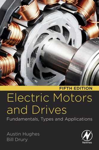
Over a very wide power range from several megawatts at the top end down to a only a few watts, all d.c. machines have the same basic structure, as shown in Fig. 3.1.
The motor has two separate electrical circuits. The smaller pair of terminals (designated E1, E2, with E for excitation—see later Fig. 3.6) connect to the field windings, which surround each pole and are normally in series: these windings provide the m.m.f. to set up the flux in the air-gap under the poles. In the steady state all the input power to the field windings is dissipated as heat—none of it is converted to mechanical output power.
The main terminals (designated A1, A2, with A for ‘armature’) convey the ‘torque-producing’ or ‘work’ current to the brushes which make sliding contact (via the commutator) with the conductors that form the so-called ‘armature’ winding on the rotor. The supply to the field (the flux-producing part of the motor) is separate from that for the armature, hence the description ‘separately excited’.
As in any electrical machine it is possible to design a d.c. motor for any desired supply voltage, but for several reasons it is unusual to find rated voltages lower than about 6 V or much higher than 700 V. The lower limit arises because the brushes (see below) give rise to an unavoidable volt-drop of perhaps 0.5–1 V, and it is clearly not good practice to let this ‘wasted’ voltage became a large fraction of the supply voltage. At the other end of the scale it becomes prohibitively expensive to insulate the commutator segments to withstand higher voltages. The function and operation of the commutator is discussed later, but it is appropriate to mention here that brushes and commutators are troublesome at very high speeds. Small d.c. motors, say up to hundreds of Watts output, can run at perhaps 12,000 rev/min, but the majority of medium and large motors are usually designed for speeds below 3000 rev/min.
Motors are usually supplied with power electronic drives, which draw power from the a.c. utility supply and convert it to d.c. for the motor. Since the utility voltages tend to be standardised (e.g. 110 V, 200–240 V, or 380–480 V, 50 or 60 Hz), motors are made with rated voltages which match the range of d.c. outputs from the converter (see Chapter 2).
As mentioned above, it is quite normal for a motor of a given power, speed and size to be available in a range of different voltages. In principle all that has to be done is to alter the number of turns and the size of wire making up the coils in the machine. A 12 V, 4 A motor, for example, could easily be made to operate from 24 V instead, by winding its coils with twice as many turns of wire having only half the cross-sectional area of the original. The full speed would be the same at 24 V as the original was at 12 V, and the rated current would be 2 A, rather than 4 A. The input power and output power would be unchanged, and externally there would be no change in appearance, except that the terminals might be a bit smaller.
Traditionally d.c. motors were classified as shunt, series, or separately excited. In addition it was common to see motors referred to as ‘compound-wound’. These descriptions date from the period before the advent of power electronics: they reflect the way in which the field and armature circuits are interconnected, which in turn determines the operating characteristics. For example, the series motor has a high starting torque when switched directly on line, so it became the natural choice for traction applications, while applications requiring constant speed would use the shunt connected motor.
However, at the fundamental level there is really no difference between the various types, so we focus attention on the separately-excited machine, before taking a brief look at shunt and series motors. Later, in Chapter 4, we will see how the operating characteristics of the separately-excited machine with power electronic supplies equip it to suit any application, and thereby displace the various historic predecessors.
We should make clear at this point that whereas in an a.c. machine the number of poles is of prime importance in determining the speed, the pole-number in a d.c. machine is of little consequence as far as the user is concerned. It turns out to be more economical to use two or four poles (perhaps with a square stator frame) in small or medium size d.c. motors, and more (e.g. 10 or 12 or even more) in large ones, but the only difference to the user is that the two-pole type will have two brushes displaced by 180°, the four-pole will have four brushes displaced by 90°, and so on. Most of our discussion centres on the two-pole version in the interests of simplicity, but there is no essential difference as far as operating characteristics are concerned.
Finally, before we move on, we should point out that confusion can be caused when people describe a type of a.c. motor which is fed from a power electronic converter with a three phase square wave voltage waveform as a ‘Brushless d.c. motor’. We suggest that the reader should forget about that at the moment—we will pick it up in Chapter 9.
3.2 Torque production
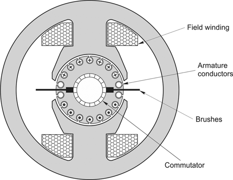
Torque is produced by interaction between the axial current-carrying conductors on the rotor and the radial magnetic flux produced by the stator. The flux or ‘excitation’ can be furnished by permanent magnets (Fig. 3.2A) or by means of field windings (Figs. 3.1 and 3.2B).
Permanent magnet versions are available in motors with outputs from a few watts up to a few kilowatts, while wound-field machines begin at about 100 watts and extend to the largest (MW) outputs. The advantages of the permanent magnet type are that no electrical supply is required for the field, and the overall size of the motor can be smaller. On the other hand the strength of the field cannot be varied so one possible option for control is ruled out.
Ferrite magnets have been used for many years. They are relatively cheap and easy to manufacture but their energy product (a measure of their effectiveness as a source of excitation) is poor. Rare earth magnets (e.g. Neodynium-iron-boron or Samarium cobalt) provide much higher energy products, and yield high torque/volume ratios: they are used in high performance servo motors, but are relatively expensive and difficult to manufacture and handle. Nd-Fe-B magnets have the highest energy product but have a modest Curie point, above which demagnetisation occurs, which may be a consideration for some demanding applications.
Although the magnetic field is essential to the operation of the motor, we should recall that in Chapter 1 we saw that none of the mechanical output power actually comes from the field system. The excitation acts like a catalyst in a chemical reaction, making the energy conversion possible but not contributing to the output.
The main (power) circuit consists of a set of identical coils wound in slots on the rotor, and known as the armature. Current is fed into and out of the rotor via carbon ‘brushes’ which make sliding contact with the commutator, which consists of insulated copper segments mounted on a cylindrical former. (The term ‘brush’ stems from the early attempts to make sliding contacts using bundles of wires bound together in much the same way as the willow twigs in a witch’s broomstick. Not surprisingly these primitive brushes soon wore grooves in the commutator.)
The function of the commutator is discussed below, but it is worth stressing here that all the electrical energy which is to be converted into mechanical output has to be fed into the motor through the brushes and commutator. Given that a high-speed sliding electrical contact is involved, it is not surprising that to ensure trouble-free operation the commutator needs to be kept clean, and the brushes and their associated springs need to be regularly serviced. Brushes wear away, of course, though if the correct ‘grade’ of brush is used and they are properly ‘bedded in’ they can last for many thousands of hours. As a very broad rule of thumb, a commutator brush could be expected to wear at a rate of 3–4000 h per centimetre. All being well, the brush debris (in the form of graphite particles) will be carried out of harm’s way by the ventilating air: any build up of dust on the insulation of the windings of a high-voltage motor risks the danger of short-circuits, while debris on the commutator itself is dangerous and can lead to disastrous ‘flashover’ faults.
The axial length of the commutator depends on the current it has to handle. Small motors usually have one brush on each side of the commutator, so the commutator is quite short, but larger heavy-current motors may well have many brushes mounted on a common arm, each with its own brushbox (in which it is free to slide) and with all the brushes on one arm connected in parallel via their flexible copper leads or ‘pigtails’. The length of the commutator can then be comparable with the ‘active’ length of the armature (i.e. the part carrying the conductors exposed to the radial flux).
3.2.1 Function of the commutator
Many different winding arrangements are used for d.c. armatures, and it is neither helpful or necessary for us to delve into the nitty-gritty of winding and commutator design. These are matters which are best left to motor designers and repairers. What we need to do is to focus on what a well designed commutator winding actually achieves, and despite the apparent complexity, this can be stated quite simply.
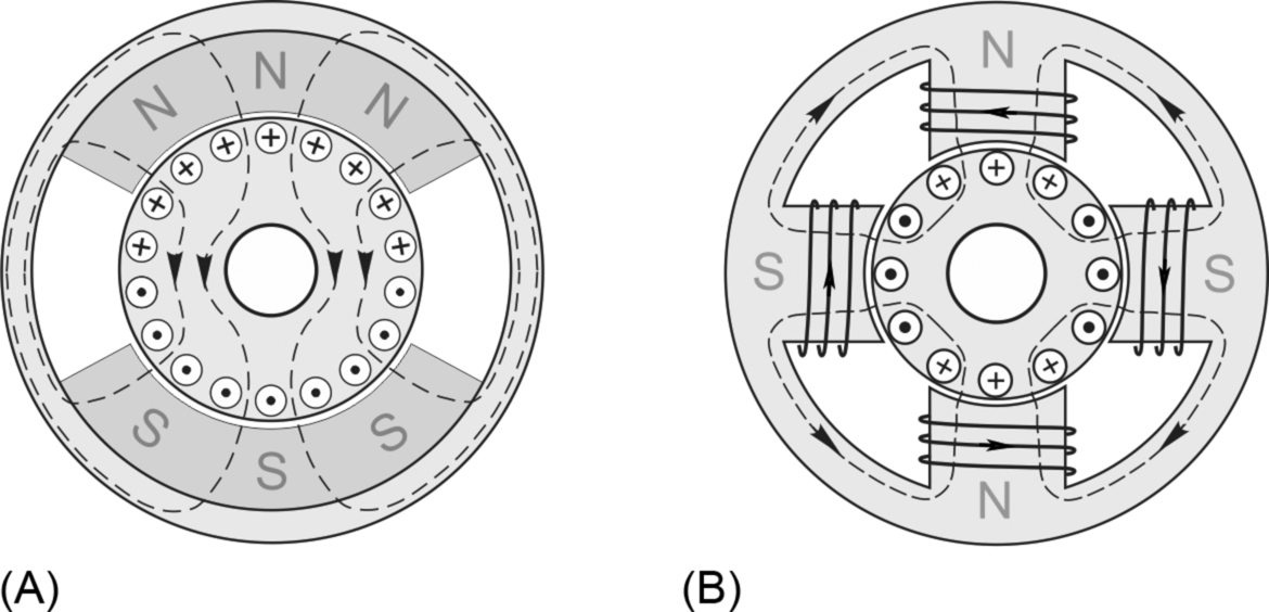
The purpose of the commutator is to ensure that regardless of the position of the rotor, the pattern of current flow in the rotor is always as shown in Fig. 3.3.
Current enters the rotor via one brush, flows through the rotor coils in the directions shown in Fig. 3.3, and leaves via the other brush. The first point of contact with the armature is via the commutator segment or segments on which the brush is pressing at the time (the brush is usually wider than a single segment), but since the interconnections between the individual coils are made at each commutator segment, the current actually passes through all the coils via all the commutator segments in its path through the armature.
We can see from Fig. 3.3 that all the conductors lying under the N pole carry current in one direction, while all those under the S pole carry current in the opposite direction. All the conductors under the N pole will therefore experience a downward force (which is proportional to the radial flux density B and the armature current I) while all the conductors under the S pole will experience an equal upward force—remember Flemings left hand rule—Fig. 1.4. A torque is thus produced on the rotor, the magnitude of the torque being proportional to the product of the flux density and the current. In practice the flux density will not be completely uniform under the pole, so the force on some of the armature conductors will be greater than on others. However, it is straightforward to show that the total torque developed is given by
where Φ is the total flux produced by the field, and KT is constant for a given motor. In the majority of motors the flux remains constant, so we see that the motor torque is directly proportional to the armature current. This extremely simple result means that if a motor is required to produce constant torque at all speeds, we simply have to arrange to keep the armature current constant. Standard drive packages usually include provision for doing this, as will be seen later. We can also see from Eq. (3.1) that the direction of the torque can be reversed by reversing either the armature current (I) or the flux (Φ). We obviously make use of this when we want the motor to run in reverse, and sometimes when we want regenerative braking.
The alert reader might rightly challenge the claim—made above—that the torque will be constant regardless of rotor position. Looking at Fig. 3.3, it should be clear that if the rotor turned just a few degrees, one of the five conductors shown as being under the pole will move out into the region where there is no radial flux, before the next one moves under the pole. Instead of five conductors producing force, there will then be only four, so won’t the torque be reduced accordingly?
The answer to this question is yes, and it is to limit this unwelcome variation of torque that most motors have many more coils than are shown in Fig. 3.3. Smooth torque is of course desirable in most applications in order to avoid vibrations and resonances in the transmission and load, and is essential in machine tool drives where the quality of finish can be marred by uneven cutting if the torque and speed are not steady.
Broadly speaking the higher the number of coils (and commutator segments) the better, because the ideal armature would be one in which the pattern of current on the rotor corresponded to a ‘current sheet’, rather than a series of discrete packets of current. If the number of coils was infinite, the rotor would look identical at every position, and the torque would therefore be absolutely smooth. Obviously this is not practicable, but it is closely approximated in most d.c. motors. For practical and economic reasons the number of slots is higher in large motors, which may well have a hundred or more coils and hence very little ripple in their output torque.
3.2.2 Operation of the commutator—interpoles
Returning now to the operation of the commutator, and focusing on a particular coil (e.g. the one shown as ab in Fig. 3.3) we note that for half a revolution—while side a is under the N pole and side b is under the S pole, the current needs to be positive in side a and negative in side b in order to produce a positive torque. For the other half revolution, while side a is under the S pole and side b is under the N pole, the current must flow in the opposite direction through the coil for it to continue to produce positive torque. This reversal of current takes place in each coil as it passes through the interpolar axis, the coil being ‘switched-round’ by the action of the commutator sliding under the brush. Each time a coil reaches this position it is said to be undergoing commutation, and the relevant coil in Fig. 3.3 has therefore been shown as having no current to indicate that its current is in the process of changing from positive to negative.
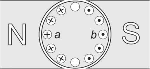
The essence of the current-reversal mechanism is revealed by the simplified sketch shown in Fig. 3.4. This diagram shows a single coil fed via the commutator and brushes with current that always flows in at the top brush.
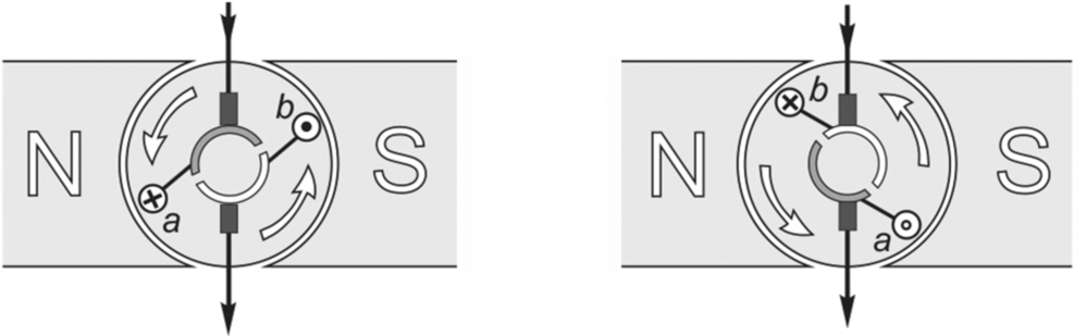
In the left-hand sketch, coil-side a is under the ![]() pole and carries positive current because it is connected to the shaded commutator segment which in turn is fed from the top brush. Side a is therefore exposed to a flux density directed from left (
pole and carries positive current because it is connected to the shaded commutator segment which in turn is fed from the top brush. Side a is therefore exposed to a flux density directed from left (![]() ) to right (
) to right (![]() ) in the sketch, and will therefore experience a downward force. This force will remain constant while the coil-side remains under the
) in the sketch, and will therefore experience a downward force. This force will remain constant while the coil-side remains under the ![]() pole. Conversely, side b has negative current but it also lies in a flux density directed from right to left, so it experiences an upward force. There is thus an anti-clockwise torque on the rotor.
pole. Conversely, side b has negative current but it also lies in a flux density directed from right to left, so it experiences an upward force. There is thus an anti-clockwise torque on the rotor.
When the rotor turns to the position shown in the sketch on the right, the current in both sides is reversed, because side b is now fed with positive current via the unshaded commutator segment. The direction of force on each coil side is reversed, which is exactly what we want in order for the torque to remain clockwise. Apart from the short period when the coil is outside the influence of the flux, and undergoing commutation (current-reversal) the torque is constant.
It should be stressed that the discussion above is intended to illustrate the principle involved, and the sketch should not be taken too literally. In a real multi-coil armature, the commutator arc is much smaller than that shown in Fig. 3.4 and only one of the many coils coil is reversed at a time, so the torque remains very nearly constant regardless of the position of the rotor.
The main difficulty in achieving good commutation arises because of the self-inductance of the armature coils, and the associated stored energy. As we have seen earlier, inductive circuits tend to resist change of current, and if the current reversal has not been fully completed by the time the brush slides off the commutator segment in question there will be a spark at the trailing edge of the brush.
In small motors some sparking is considered tolerable, but in medium and large wound-field motors small additional stator poles known as interpoles (or compoles) are provided to improve commutation and hence minimise sparking. These extra poles are located midway between the main field poles, as shown in Fig. 3.5. Interpoles are not normally required in permanent magnet motors because the absence of stator iron close to the rotor coils results in much lower armature coil inductance.

The purpose of the interpoles is to induce a motional e.m.f. in the coil undergoing commutation, in such a direction as to speed-up the desired reversal of current, and thereby prevent sparking. The e.m.f. needed is proportional to the current which has to be commutated, i.e. the armature current, and to the speed of rotation. The correct e.m.f. is therefore achieved by passing the armature current through the coils on the interpoles, thereby making the flux from the interpoles proportional to the armature current. The interpole coils therefore consist of a few turns of thick conductor, connected permanently in series with the armature.
3.3 Motional e.m.f.
Readers who have skipped Chapter 1 are advised to check that they are familiar with the material covered in Section 1.7 before reading the rest of this chapter, as not all of the lessons drawn in Chapter 1 are repeated explicitly here.
When the armature is stationary, no motional e.m.f. is induced in it. But when the rotor turns, the armature conductors cut the radial magnetic flux and an e.m.f. is induced in them.
As far as each individual coil on the armature is concerned, an alternating e.m.f. will be induced in it when the rotor rotates. For the coil ab in Fig. 3.3, for example, side a will be moving upward through the flux if the rotation is clockwise, and an e.m.f. directed out of the plane of the paper will be generated. At the same time the ‘return’ side of the coil (b) will be moving downwards, so the same magnitude of e.m.f. will be generated, but directed into the paper. The resultant e.m.f. in the coil will therefore be twice that in the coil-side, and this e.m.f. will remain constant for almost half a revolution, during which time the coil sides are cutting a constant flux density. For the comparatively short time when the coil is not cutting any flux the e.m.f. will be zero, and then the coil will begin to cut through the flux again, but now each side is under the other pole, so the e.m.f. is in the opposite direction. The resultant e.m.f. waveform in each coil is therefore a rectangular alternating wave, with magnitude and frequency proportional to the speed of rotation.
The coils on the rotor are connected in series, so if we were to look at the e.m.f. across any given pair of diametrically opposite commutator segments, we would see a large alternating e.m.f. (We would have to station ourselves on the rotor to do this, or else make sliding contacts using slip-rings).
The fact that the induced voltage in the rotor is alternating may come as a surprise, since we are talking about a d.c. motor rather than an a.c. one. But any worries we may have should be dispelled when we ask what we will see by way of induced e.m.f. when we ‘look in’ at the brushes. We will see that the brushes and commutator effect a remarkable transformation, bringing us back into the reassuring world of d.c.
The first point to note is that the brushes are stationary. This means that although a particular segment under each brush is continually being replaced by its neighbour, the circuit lying between the two brushes always consists of the same number of coils, with the same orientation with respect to the poles. As a result the e.m.f. at the brushes is direct (i.e. constant), rather than alternating.
The magnitude of the e.m.f. depends on the position of the brushes around the commutator, but they are invariably placed at the point where they continually ‘see’ the peak value of the alternating e.m.f. induced in the armature. In effect, the commutator and brushes can be regarded as a mechanical rectifier which converts the alternating e.m.f. in the rotating reference frame to a direct e.m.f. in the stationary reference frame. It is a remarkably clever and effective device, its only real drawback being that it is a mechanical system, and therefore subject to wear and tear.
We saw earlier that to obtain smooth torque it was necessary for there to be a large number of coils and commutator segments, and we find that much the same considerations apply to the smoothness of the generated e.m.f. If there are only a few armature coils the e.m.f. will have a noticeable ripple superimposed on the mean d.c. level. The higher we make the number of coils, the smaller the ripple, and the better the d.c. we produce. The small ripple we inevitably get with a finite number of segments is seldom any problem with motors used in drives, but can sometimes give rise to difficulties when a d.c. machine is used to provide a speed feedback signal in a closed-loop system (see Chapter 4).
In Chapter 1 we saw that when a conductor of length l moves at velocity v through a flux density B, the motional e.m.f. induced is given by e = Blv. In the complete machine we have many series-connected conductors; the linear velocity (v) of the primitive machine examined in Chapter 1 is replaced by the tangential velocity of the rotor conductors, which is clearly proportional to the speed of rotation (n); and the average flux density cut by each conductor (B) is directly related to the total flux (Φ). If we roll together the other influential factors (number of conductors, radius, active length of rotor) into a single constant (KE), it follows that the magnitude of the resultant e.m.f. (E) which is generated at the brushes is given by
This equation reminds us of the key role of the flux, in that until we switch on the field no voltage will be generated, no matter how fast the rotor turns. Once the field is energised, the generated voltage is directly proportional to the speed of rotation, so if we reverse the direction of rotation, we will also reverse the polarity of the generated e.m.f. We should also remember that the e.m.f. depends only on the flux and the speed, and is the same regardless of whether the rotation is provided by some external source (i.e. when the machine is being driven as a generator) or when the rotation is produced by the machine itself (i.e. when it is acting as a motor).
It has already been mentioned that the flux is usually constant at its full value, in which case Eqs (3.1) and (3.2) can be written in the form
where kt is the motor torque constant, ke is the e.m.f. constant, and ω is the angular speed in rad/s.
In this book the international standard (SI) system of units is used throughout. In the SI system, the units for kt are the units of torque (Newton metre) divided by the unit of current (Ampere), i.e. Nm/A; and the units of ke are Volts/rad/s. (Note, however, that ke is more often given in Volts/1000 rev/min.)
It is not at all clear that the units for the torque constant (Nm/A) and the e.m.f. constant (V/rad/s), which on the face of it measure very different physical phenomena, are in fact the same, i.e. 1 Nm/A = 1 Volt/rad/s. Some readers will be content simply to accept it, others may be puzzled, a few may even find it obvious. Those who are surprised and puzzled may feel more comfortable by progressively replacing one set of units by their equivalent, to lead us in the direction of the other, e.g.

This still leaves us to ponder what happened to the ‘radians’ in ke, but at least the underlying unity is demonstrated, and after all a radian is a dimensionless quantity. Delving deeper, we note that 1 Volt.second = 1 Weber, the unit of magnetic flux. This is hardly surprising because the production of torque and the generation of motional e.m.f. are both brought about by the catalytic action of the magnetic flux.
Returning to more pragmatic issues, we have now discovered the extremely convenient fact that in SI units, the torque and e.m.f. constants are equal, i.e. kt = ke = k. The torque and e.m.f. equations can thus be further simplified as
We will make use of these two delightfully simple equations time and again in the subsequent discussion. Together with the armature voltage equation (see below), they allow us to predict all aspects of behaviour of a d.c. motor. There can be few such versatile machines for which the fundamentals can be expressed so simply.
Though attention has been focused on the motional e.m.f. in the conductors, we must not overlook the fact that motional e.m.f.s are also induced in the body of the rotor. If we consider a rotor tooth, for example, it should be clear that it will have an alternating e.m.f. induced in it as the rotor turns, in just the same way as the e.m.f. induced in the adjacent conductor. In the machine shown in Fig. 3.1, for example, when the e.m.f. in a tooth under a N pole is positive, the e.m.f. in the diametrically opposite tooth (under a S pole) will be negative. Given that the rotor steel conducts electricity, these e.m.f.s will tend to set up circulating currents in the body of the rotor, so to prevent this happening, the rotor is made not from a solid piece but from thin steel laminations (typically less than 1 mm thick) which have an insulated coating to prevent the flow of unwanted currents. If the rotor was not laminated the induced current would not only produce large quantities of waste heat, but also exert a substantial braking torque.
3.3.1 Equivalent circuit
The equivalent circuit can now be drawn on the same basis as we used for the primitive machine in Chapter 1, and is shown in Fig. 3.6.
The voltage V is the voltage applied to the armature terminals (i.e. across the brushes), and E is the internally developed motional e.m.f. The resistance and inductance of the complete armature are represented by R and L in Fig. 3.6. The sign convention adopted is the usual one when the machine is operating as a motor. Under motoring conditions, the motional e.m.f. E always opposes the applied voltage V, and for this reason it is referred to as ‘back e.m.f.’. For current to be forced into the motor, V must be greater than E, the armature circuit voltage equation being given by
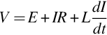
The last term in Eq. (3.7) represents the inductive volt-drop due to the armature self-inductance. This voltage is proportional to the rate of change of current, so under steady-state conditions (when the current is constant), the term will be zero and can be ignored. We will see later that the armature inductance has an unwelcome effect under transient conditions, but is also very beneficial in smoothing the current waveform when the motor is supplied by a controlled rectifier.
3.4 D.C. motor—steady-state characteristics
From the user’s viewpoint the extent to which speed falls when load is applied, and the variation in speed with applied voltage are usually the first questions which need to be answered in order to assess the suitability of the motor for the job in hand. The information is usually conveyed in the form of the steady-state characteristics, which indicate how the motor behaves when any transient effects (caused for example by a sudden change in the load) have died away and conditions have once again become steady. Steady-state characteristics are usually much easier to predict than transient characteristics, and for the d.c. machine they can all be deduced from the simple equivalent circuit in Fig. 3.6.
Under steady conditions, the armature current I is constant and Eq. (3.7) simplifies to
This equation allows us to find the current if we know the applied voltage, the speed (from which we get E via Eq. 3.6) and the armature resistance, and we can then obtain the torque from Eq. (3.5). Alternatively, we may begin with torque and speed, and work out what voltage will be needed.
We will derive the steady-state torque-speed characteristics for any given armature voltage V shortly, but first we begin by establishing the relationship between the no-load speed and the armature voltage, since this is the foundation on which the speed control philosophy is based.
3.4.1 No-load speed
By ‘no-load’ we mean that the motor is running light, so that the only mechanical resistance is that due to its own friction. In any sensible motor the frictional torque will be small, and only a small driving torque will therefore be needed to keep the motor running. Since motor torque is proportional to current (Eq. 3.5), the no-load current will also be small. If we assume that the no-load current is in fact zero, the calculation of no-load speed becomes very simple. We note from Eq. (3.8) that zero current implies that the back e.m.f. is equal to the applied voltage, while Eq. (3.2) shows that the back e.m.f. is proportional to speed. Hence under true no-load (zero torque) conditions, we obtain

where n is the speed. (We have used Eq. (3.8) for the e.m.f., rather than the simpler Eq. (3.4) because the latter only applies when the flux is at its full value, and in the present context it is important for us to see what happens when the flux is reduced.)
At this stage we are concentrating on the steady-state running speeds, but we are bound to wonder how it is that the motor reaches speed from rest. We will return to this when we look at transient behaviour, so for the moment it is sufficient to recall that we came across an equation identical to Eq. (3.9) when we looked at the primitive linear motor in Chapter 1. We saw that if there was no resisting force opposing the motion, the speed would rise until the back e.m.f. equalled the supply voltage. The same result clearly applies to the frictionless and unloaded d.c. motor here.
We see from Eq. (3.9) that the no-load speed is directly proportional to armature voltage, and inversely proportional to field flux. For the moment we will continue to consider the case where the flux is constant, and demonstrate by means of an example that the approximations used in arriving at Eq. (3.9) are justified in practice. Later, we can use the same example to study the torque-speed characteristic.
3.4.2 Performance calculation—example
Consider a 500 V, 9.1 kW, 20 A, permanent-magnet motor with an armature resistance of 1 Ω. (These values tell us that the normal operating voltage is 500 V, the current when the motor is fully loaded is 20 A, and the mechanical output power under these full-load conditions is 9.1 kW.) When supplied at 500 V, the unloaded motor is found to run at 1040 rev/min, drawing a current of 0.8 A.
Whenever the motor is running at a steady speed, the torque it produces must be equal (and opposite) to the total opposing or load torque: if the motor torque was less than the load torque, it would decelerate, and if the motor torque was higher than the load torque it would accelerate. From Eq. (3.3), we see that the motor torque is determined by its current, so we can make the important statement that, in the steady-state, the motor current will be determined by the mechanical load torque. When we make use of the equivalent circuit (Fig. 3.6) under steady-state conditions we will need to get used to the idea that the current is determined by the load torque—i.e. one of the principal ‘inputs’ which will allow us to solve the circuit equations is the mechanical load torque, which is not even shown on the diagram. For those who are not used to electromechanical interactions this can be a source of difficulty.
Returning to our example, we note that because it is a real motor, it draws a small current (and therefore produces some torque) even when unloaded. The fact that it needs to produce torque, even though no load torque has been applied and it is not accelerating, is attributable to the inevitable friction in the cooling fan, bearings and brushgear.
If we want to estimate the no-load speed at a different armature voltage (say 250 V), we would ignore the small no-load current and use Eq. (3.9), giving
Since Eq. (3.9) is based on the assumption that the no-load current is zero, this result is only approximate.
If we insist on being more precise, we must first calculate the original value of the back e.m.f., using Eq. (3.8), which gives
As expected the back e.m.f. is almost equal to the applied voltage. The corresponding speed is 1040 rev/min, so the e.m.f. constant must be 499.2/1040 or 480 Volts/1000 rev/min. To calculate the no-load speed for V = 250 Volts, we first need to know the current. We are not told anything about how the friction torque varies with speed so all we can do is to assume that the friction torque is constant, in which case the motor current will be 0.8 A regardless of speed. With this assumption, the back e.m.f. will be given by
And hence the speed will be given by

The difference between the approximate and true no-load speeds is very small, and is unlikely to be significant. Hence we can safely use Eq. (3.9) to predict the no-load speed at any armature voltage, and obtain the set of no-load speeds shown in Fig. 3.7.

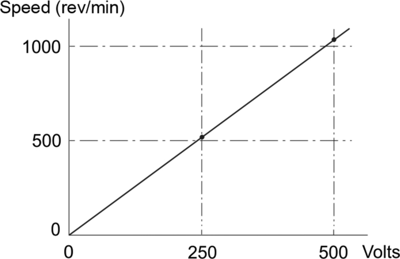
This diagram illustrates the very simple linear relationship between the speed of an unloaded d.c. motor and the armature voltage.
3.4.3 Behaviour when loaded
Having seen that the no-load speed of the motor is directly proportional to the armature voltage, we need to explore how the speed will vary when we change the load on the shaft.
The usual way we quantify ‘load’ is to specify the torque needed to drive the load at a particular speed. Some loads, such as a simple drum-type hoist with a constant weight on the hook, require the same torque regardless of speed, but for most loads the torque needed varies with the speed. For a fan, for example, the torque needed varies roughly with the square of the speed. If we know the torque/speed characteristic of the load, and the torque/speed characteristic of the motor (see below), we can find the steady-state speed simply by finding the intersection of the two curves in the torque-speed plane. An example (not specific to a d.c. motor) is shown in Fig. 3.8.

At point X the torque produced by the motor is exactly equal to the torque needed to keep the load turning, so the motor and load are in equilibrium and the speed remains steady. At all lower speeds, the motor torque will be higher than the load torque, so the net torque will be positive, leading to an acceleration of the motor. As the speed rises towards X the acceleration reduces until the speed stabilises at X. Conversely, at speeds above X the motor’s driving torque is less than the braking torque exerted by the load, so the net torque is negative and the system will decelerate until it reaches equilibrium at X. This example is one which is inherently stable, so that if the speed is disturbed for some reason from the point X, it will always return there when the disturbance is removed.
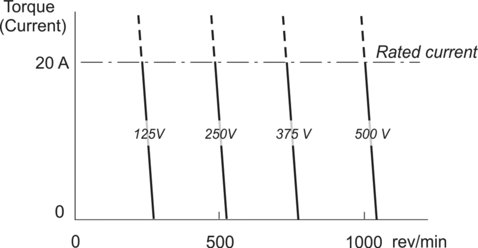
Turning now to the derivation of the torque/speed characteristics of the d.c. motor, we can profitably extend the previous example to illustrate matters. We can obtain the full-load speed for V = 500 Volts by first calculating the back e.m.f. at full load (i.e. when the current is 20 A). From Eq. (3.8) we obtain
We have already seen that the e.m.f. constant is 480 Volts/1000 rev/min, so the full load speed is clearly 1000 rev/min. From no-load to full-load the speed falls linearly, giving the torque-speed curve for V = 500 Volts shown in Fig. 3.9. Note that from no-load to full-load the speed falls from 1040 rev/min to 1000 rev/min, a drop of only 4%. Over the same range the back e.m.f. falls from very nearly 500 Volts to 480 Volts, which of course also represents a drop of 4%.
We can check the power balance using the same approach as in Section 1.7 of Chapter 1. At full load the electrical input power is given by VI, i.e. 500 V × 20 A = 10 kW. The power loss in the armature resistance is I2 R = 400 × 1 = 400 W. The power converted from electrical to mechanical form is given by EI, i.e. 480 V × 20 A = 9600 W. We can see from the no-load data that the power required to overcome friction and iron losses (eddy currents and hysteresis, mainly in the rotor) at no-load is approximately 500 V × 0.8 A = 400 W, so this leaves about 9.2 kW. The rated output power of 9.1 kW indicates that 100 W of additional losses (which we will not attempt to explore here) can be expected under full-load conditions.
Two important observations follow from these calculations. Firstly, the drop in speed when load is applied (the ‘droop’) is very small. This is very desirable for most applications, since all we have to do to maintain almost constant speed is to set the appropriate armature voltage and keep it constant. Secondly, a delicate balance between V and E is revealed. The current is in fact proportional to the difference between V and E (Eq. 3.8), so that quite small changes in either V or E give rise to disproportionately large changes in the current. In the example, a 4% reduction in E causes the current to rise to its rated value. Hence to avoid excessive currents (which cannot be tolerated in a thyristor supply, for example), the difference between V and E must be limited. This point will be taken up again when transient performance is explored.
A representative family of torque-speed characteristics for the motor discussed above is shown in Fig. 3.9. As already explained, the no-load speeds are directly proportional to the applied voltage, while the slope of each curve is the same, being determined by the armature resistance: the smaller the resistance the less the speed falls with load. These operating characteristics are very attractive because the speed can be set simply by applying the correct voltage.
The upper region of each characteristic in Fig. 3.9 is shown dotted because in this region the armature current is above its rated value, and therefore the motor cannot be operated continuously without overheating. Motors can and do operate for short periods above rated current, and the fact that the d.c. machine can continue to provide torque in proportion to current well into the overload region makes it particularly well-suited to applications requiring the occasional boost of excess torque.
A cooling problem might be expected when motors are run continuously at full current (i.e. full torque) even at very low speed, where the natural ventilation is poor. This operating condition is considered quite normal in converter-fed motor drive systems, and motors are accordingly fitted with a small air-blower motor as standard.
This book is about motors, which convert electrical power into mechanical power. But, in common with all electrical machines, the d.c. motor is inherently capable of operating as a generator, converting mechanical power into electrical power. And although the overwhelming majority of d.c. machines will spend most of their time in motoring mode, there are applications such as rolling mills where frequent reversal is called for, and others where rapid braking is required. In the former, the motor is controlled so that it returns the stored kinetic energy to the supply system each time the rolls have to be reversed, while in the latter case the energy may also be returned to the supply, or dumped as heat in a resistor. These transient modes of operation during which the machine acts as a generator may better be described as ‘regeneration’ since they only involve recovery of mechanical energy that was originally provided by the motor.
Continuous generation is of course possible using a d.c. machine provided we have a source of mechanical power, such as an internal combustion engine. In the example discussed above we saw that when connected to a 500 V supply, the unloaded machine ran at 1040 rev/min, at which point the back e.m.f. was very nearly 500 V and only a tiny positive current was flowing. As we applied mechanical load to the shaft the steady-state speed fell, thereby reducing the back e.m.f. and increasing the armature current until the motor torque was equal to the opposing load torque and equilibrium returned.
Conversely, if instead of applying an opposing (load) torque, we use the IC engine to supply torque in the opposite direction, i.e. trying to increase the speed of the motor, the increase in speed will cause the motional e.m.f. to be greater than the supply voltage (500 V). This means that the current will flow from the d.c. machine to the supply, resulting in a negative torque and reversal of electrical power flow back into the supply. Stable generating conditions will be achieved when the motor torque (current) is equal and opposite to the torque provided by the IC engine. In the example, the full-load current is 20 A, so in order to drive this current through its own resistance and overcome the supply voltage the e.m.f. must be given by
The corresponding speed can be calculated by reference to the no-load e.m.f. (499.2 Volts at 1040 rev/min) from which the steady generating speed is given by

On the torque-speed plot (Fig. 3.9) this condition lies on the downward projection of the 500 V characteristic at a current of − 20 A. We note that the full range of operation, from full-load motoring to full-load generating is accomplished with only a modest change in speed from 1000 to 1083 rev/min.
It is worth emphasising that in order to make the unloaded motor move into the generating mode, all that we had to do was to start supplying mechanical power to the motor shaft. No physical changes had to be made to the motor to make it into a generator—the hardware is equally at home functioning as a motor or as a generator—which is why it is best referred to as a ‘machine’. An electric vehicle takes full advantage of this inherent reversibility, recharging the battery when we decelerate or descend a hill. (How nice it would be if the internal combustion engine could do the same; whenever we slowed down, we could watch the rising gauge as our kinetic energy was converted back into hydrocarbon fuel in the tank!)
To complete this section we will derive the analytical expression for the steady-state speed as a function of the two variables that we can control, i.e. the applied voltage (V), and the load torque (TL). Under steady-state conditions the armature current is constant and we can therefore ignore the armature inductance term in Eq. (3.7); and because there is no acceleration, the motor torque is equal to the load torque. Hence by eliminating the current I between Eqs (3.5) and (3.7), and substituting for E from Eq. (3.6) the speed is given by

This equation represents a straight line in the speed/torque plane, as we saw with our previous worked example. The first term shows that the no-load speed is directly proportional to the armature voltage, while the second term gives the drop in speed for a given load torque. The gradient or slope of the torque-speed curve is –![]() , showing again that the smaller the armature resistance, the smaller the drop in speed when load is applied.
, showing again that the smaller the armature resistance, the smaller the drop in speed when load is applied.
3.4.4 Base speed and field weakening
Returning to our consideration of motor operating characteristics, when the field flux is at its full value the speed corresponding to full armature voltage and full current (i.e. the rated full-load condition) is known as base speed (see Fig. 3.10). The upper part of the figure shows the regions of the torque speed plane within which the motor can operate without exceeding its maximum or rated current. The lower diagram shows the maximum output power as a function of speed.
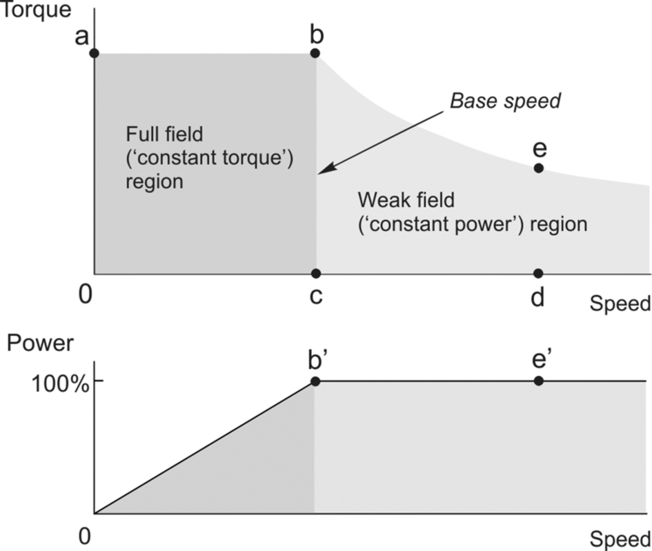
The motor can operate at any speed up to base speed, and any torque (current) up to rated value by appropriate choice of armature voltage. This full flux region of operation is indicated by the shaded area Oabc in Fig. 3.10, and is often referred to as the ‘constant torque’ region of the torque-speed characteristic. In this context ‘constant torque’ signifies that at any speed below base speed the motor is capable of producing its full rated torque. Note that the term constant torque does not mean that the motor will produce constant torque, but rather it signifies that the motor can produce constant torque if required: as we have already seen, it is the mechanical load we apply to the shaft that determines the steady-state torque produced by the motor.
When the current is at maximum (i.e. along the line ab in Fig. 3.10), the torque is at its maximum (rated) value. Since mechanical power is given by torque times speed, the power output along ab is proportional to the speed, as shown in the lower part of the figure, and the maximum power thus corresponds to the point b in Fig. 3.10. At point b both the voltage and current have their full rated values.
To run faster than base speed the field flux must be reduced, as indicated by Eq. (3.9). Operation with reduced flux is known as ‘field weakening’, and we have already discussed this perhaps surprising mode in connection with the primitive linear motor in Chapter 1. For example by halving the flux (and keeping the armature voltage at its full value), the no-load speed is doubled (point d in Fig. 3.10). The increase in speed is however obtained at the expense of available torque, which is proportional to flux times current (see Eq. 3.1). The current is limited to rated value, so if the flux is halved, the speed will double but the maximum torque which can be developed is only half the rated value (point e in Fig. 3.10). Note that at the point e both the armature voltage and the armature current again have their full rated values, so the power is at maximum, as it was at point b. The power is constant along the curve through b and e, and for this reason the shaded area to the right of the line bc is referred to as the ‘constant power’ region. Obviously, field weakening is only satisfactory for applications which do not demand full torque at high speeds, such as electric traction.
The maximum allowable speed under weak field conditions must be limited (to avoid excessive sparking at the commutator), and is usually indicated on the motor rating plate. A marking of 1200/1750 rev/min, for example, would indicate a base speed of 1200 rev/min, and a maximum speed with field weakening of 1750 rev/min. The field weakening range varies widely depending on the motor design, but maximum speed rarely exceeds three or four times base speed.
To sum up, the speed is controlled as follows:
- • Below base speed, the flux is maximum, and the speed is set by the armature voltage. Full torque is available at any speed.
- • Above base speed the armature voltage is at (or close to) maximum, and the flux is reduced in order to raise the speed. The maximum torque available reduces in proportion to the flux.
To judge the suitability of a motor for a particular application we need to compare the torque-speed characteristic of the prospective load with the operating diagram for the motor: if the load torque calls for operation outside the shaded areas of Fig. 3.10, a larger motor is clearly called for.
Finally, we should note that according to Eq. (3.9), the no-load speed will become infinite if the flux is reduced to zero. This seems an unlikely state of affairs: after all, we have seen that the field is essential for the motor to operate, so it seems unreasonable to imagine that if we removed the field altogether, the speed would rise to infinity. In fact, the explanation lies in the assumption that ‘no-load’ for a real motor means zero torque. If we could make a motor which had no friction torque whatsoever, the speed would indeed continue to rise as we reduced the field flux towards zero. But as we reduced the flux, the torque per ampere of armature current would become smaller and smaller, so in a real machine with friction, there will come a point where the torque being produced by the motor is equal to the friction torque, and the speed will therefore be limited. Nevertheless, it is quite dangerous to open-circuit the field winding, especially in a large unloaded motor. There may be sufficient ‘residual’ magnetism left in the poles to produce significant accelerating torque to lead to a run-away situation. Usually, field and armature circuits are interlocked so that if the field is lost, the armature circuit is switched off automatically.
3.4.5 Armature reaction
In addition to deliberate field-weakening, as discussed above, the flux in a d.c. machine can be weakened by an effect known as ‘armature reaction’. As its name implies, armature reaction relates to the influence that the armature m.m.f. has on the flux in the machine: in small machines it is negligible, but in large machines the unwelcome field weakening caused by armature reaction is sufficient to warrant extra design features to combat it. A full discussion would be well beyond the needs of most users, but a brief explanation is included for the sake of completeness.
The way armature reaction occurs can best be appreciated by looking at Fig. 3.1 and noting that the m.m.f. of the armature conductors acts along the axis defined by the brushes, i.e. the armature m.m.f. acts in quadrature to the main flux axis which lies along the stator poles. The reluctance in the quadrature direction is high because of the large air spaces that the flux has to cross, so despite the fact that the rotor m.m.f. at full current can be very large, the quadrature flux is relatively small; and because it is perpendicular to the main flux, the average value of the latter would not be expected to be affected by the quadrature flux, even though part of the path of the reaction flux is shared with the main flux as it passes (horizontally in Fig. 3.1) through the main pole-pieces.
A similar matter was addressed in relation to the primitive machine in Chapter 1. There it was explained that it was not necessary to take account of the flux produced by the conductor itself when calculating the electromagnetic force on it. And if it were not for the non-linear phenomenon of magnetic saturation, the armature reaction flux would have no effect on the average value of the main flux in the machine shown in Fig. 3.1: the flux density on one edge of the pole-pieces would be increased by the presence of the reaction flux, but decreased by the same amount on the other edge, leaving the average of the main flux unchanged. However if the iron in the main magnetic circuit is already some way into saturation, the presence of the rotor m.m.f. will cause less of an increase on the one edge than it causes by way of decrease on the other, and there will be a net reduction in main flux.
We know that reducing the flux leads to an increase in speed, so we can now see that in a machine with pronounced armature reaction, when the load on the shaft is increased and the armature current increases to produce more torque, the field is simultaneously reduced and the motor speeds up. Though this behaviour is not a true case of instability, it is not generally regarded as desirable!
Large motors often carry additional windings fitted into slots in the pole-faces and connected in series with the armature. These ‘compensating’ windings produce an m.m.f. in opposition to the armature m.m.f., thereby reducing or eliminating the armature reaction effect.
3.4.6 Maximum output power
We have seen that if the mechanical load on the shaft of the motor increases, the speed falls and the armature current automatically increases until equilibrium of torque is reached and the speed again becomes steady. If the armature voltage is at its maximum (rated) value, and we increase the mechanical load until the current reaches its rated value, we are clearly at full-load, i.e. we are operating at the full speed (determined by voltage) and the full torque (determined by current). The maximum current is set at the design stage, and reflects the tolerable level of heating of the armature conductors.
Clearly if we increase the load on the shaft still more, the current will exceed the safe value, and the motor will begin to overheat. But the question which this prompts is ‘if it were not for the problem of overheating, could the motor deliver more and more power output, or is there a limit’?
We can see straightaway that there will be a maximum by looking at the torque-speed curves in Fig. 3.9. The mechanical output power is the product of torque and speed, and we see that the power will be zero when either the load torque is zero (i.e. the motor is running light) or the speed is zero (i.e. the motor is stationary). There must be maximum between these two zeroes, and it is easy to show that the peak mechanical power occurs when the speed is half of the no-load speed. However, this operating condition is only practicable in very small motors: in the majority of motors, the supply would simply not be able to supply the very high current required.
Turning to the question of what determines the theoretical maximum power, we can apply the maximum power transfer theorem (from circuit theory) to the equivalent circuit in Fig. 3.6. The inductance can be ignored because we assume d.c. conditions. If we regard the armature resistance R as if it were the resistance of the source V, the theorem tells us that in order to transfer maximum power to the load (represented by the motional e.m.f. on the right-hand side of Fig. 3.6) we must make the load ‘look like’ a resistance equal to the source resistance, R. This condition is obtained when the applied voltage V divides equally so that half of it is dropped across R and the other half is equal to the e.m.f., E. (We note that the condition E = V/2 corresponds to the motor running at half the no-load speed, as stated above.) At the maximum power point, the current is V/2R, and the mechanical output power (EI) is given by V2/4R.
The expression for the maximum output power is delightfully simple. We might have expected the maximum power to depend on other motor parameters, but in fact it is determined solely by the armature voltage and the armature resistance. For example, we can say immediately that a 12 V motor with an armature resistance of 1 Ω cannot possibly produce more than 36 W of mechanical output power.
We should of course observe that under maximum power conditions the overall efficiency is only 50% (because an equal power is burned off as heat in the armature resistance); and emphasise again that only very small motors can ever be operated continuously in this condition. For the vast majority of motors, it is of academic interest only, because the current (V/2R) will be far too high for the supply.
3.5 Transient behaviour
It has already been pointed out that the steady-state armature current depends on the small difference between the back e.m.f. E and the applied voltage V. In a converter-fed drive it is vital that the current is kept within safe bounds, otherwise the thyristors or transistors (which have very limited overcurrent capacity) will be destroyed, and it follows from Eq. (3.8) that in order to prevent the current from exceeding its rated value we cannot afford to let V and E differ by more than IR, where I is the rated current.
It would be unacceptable, for example, to attempt to bring all but the smallest of d.c. motors up to speed simply by switching on rated voltage. In the example studied earlier, rated voltage is 500 V, and the armature resistance is 1 Ω. At standstill the back e.m.f. is zero, and hence the initial current would be 500/1 = 500 A, or 25 times rated current! This would destroy the thyristors in the supply converter (and/or blow the fuses). Clearly the initial voltage we must apply is much less than 500 V; and if we want to limit the current to rated value (20 A in the example) the voltage needed will be 20 × 1, i.e. only 20 Volts. As the speed picks up, the back e.m.f. rises, and to maintain the full current V must also be ramped up so that the difference between V and E remains constant at 20 V. Of course, the motor will not accelerate nearly so rapidly when the current is kept in check as it would if we had switched on full voltage, and allowed the current to do as it pleased. But this is the price we must pay in order to protect the converter.
Similar current-surge difficulties occur if the load on the motor is suddenly increased, because this will result in the motor slowing down, with a consequent fall in E. In a sense we welcome the fall in E because this is what brings about the increase in current needed to supply the extra load, but of course we only want the current to rise to its rated value: beyond that point we must be ready to reduce V, to prevent an excessive current.
The solution to the problem of overcurrents lies in providing closed-loop current-limiting as an integral feature of the motor/drive package. The motor current is sensed, and the voltage V is automatically adjusted so that rated current is not exceeded continuously, although typically it is allowed to reach 1.5 times rated current for up to 60 s. We will discuss the current control loop in Chapter 4.
3.5.1 Dynamic behaviour and time-constants
The use of the terms ‘surge’ and ‘sudden’ in the discussion above will doubtless have created the impression that changes in the motor current or speed can take place instantaneously, whereas in fact a finite time is always necessary to effect changes in either. (If the current changes, then so does the stored energy in the armature inductance; and if speed changes, so does the rotary kinetic energy stored in the inertia. For either of these changes to take place in zero time it would be necessary for there to be a pulse of infinite power, which is clearly impossible.)
The theoretical treatment of the transient dynamics of the d.c. machine is easier than for any other type of electric motor but is nevertheless beyond our scope. However it is worth summarising the principal features of the dynamic behaviour, and highlighting the fact that all the transient changes that occur are determined by only two time-constants. The first (and most important from the user’s viewpoint) is the electromechanical time-constant, which governs the way the speed settles to a new level following a disturbance such as a change in armature voltage or load torque. The second is the electrical (or armature) time-constant, which is usually much shorter and governs the rate of change of armature current immediately following a change in armature voltage.
When the motor is running, there are two ‘inputs’ that we can change suddenly, namely the applied voltage and the load torque. When either of these is changed, the motor enters a transient period before settling to its new steady state. It turns out that if we ignore the armature inductance (i.e. we take the armature time-constant to be zero), the transient period is characterised by first-order exponential responses in the speed and current. This assumption is valid for all but the very largest motors. We obtained a similar result when we looked at the primitive linear motor in Chapter 1 (see Fig. 1.16).
For example, if we suddenly increased the armature voltage of a frictionless and unloaded motor from V1 to V2, its speed and current would vary as shown in Fig. 3.11.

There is an immediate increase in the current (because we have ignored the inductance), reflecting the fact that the applied voltage is suddenly more than the back e.m.f.; the increased current produces more torque and hence the motor accelerates; the rising speed is accompanied by an increase in back e.m.f., so the current begins to fall; and the process continues until a new steady speed is reached corresponding to the new voltage. In this particular case the steady-state current is zero because we have assumed that there is no friction or load torque, but the shape of the dynamic response would be the same if there had been an initial load, or if we had suddenly changed the load.
The expression describing the current as a function of time (t) is:-

The expression for the change in speed is similar, the time dependence again featuring the exponential transient term, ![]() . The significance of the time-constant (τ) is shown in Fig. 3.11. If the initial gradient of the current-time graph is projected it intersects the final value after one time-constant. In theory, it takes an infinite time for the response to settle, but in practice the transient is usually regarded as over after about 4 or 5 time-constants. We note that the transient response is very satisfactory: as soon as the voltage is increased the current immediately increases to provide more torque and begin the acceleration, but the accelerating torque is reduced progressively to ensure that the new target speed is approached smoothly. Happily, because the system is first-order, there is no suggestion of an oscillatory response with overshoots.
. The significance of the time-constant (τ) is shown in Fig. 3.11. If the initial gradient of the current-time graph is projected it intersects the final value after one time-constant. In theory, it takes an infinite time for the response to settle, but in practice the transient is usually regarded as over after about 4 or 5 time-constants. We note that the transient response is very satisfactory: as soon as the voltage is increased the current immediately increases to provide more torque and begin the acceleration, but the accelerating torque is reduced progressively to ensure that the new target speed is approached smoothly. Happily, because the system is first-order, there is no suggestion of an oscillatory response with overshoots.
Analysis yields the relationship between the time-constant and the motor/system parameters as

where R is the armature resistance, J is the total rotary inertia of motor plus load, and k is the motor constant (Eqs 3.3 and 3.4). The appropriateness of the term ‘electromechanical time-constant’ should be clear from Eq. (3.12), because τ depends on the electrical parameters (R and k) and the mechanical parameter, J. The fact that if the inertia was doubled, the time-constant would double and transients would take twice as long is perhaps to be expected, but the influence of the motor parameters R and k is probably not so obvious.
The electrical or armature time-constant is defined in the usual way for a series L, R circuit, i.e.
If we were to hold the rotor of a d.c. motor stationary and apply a step voltage V to the armature, the current would climb exponentially to a final value of V/R with a time-constant τa .
If we always applied pure d.c. voltage to the motor we would probably want τa to be as short as possible, so that there was no delay in the build-up of current when the voltage is changed.
But given that most motors are fed with voltage waveforms which are far from smooth (see Chapter 2), we are actually rather pleased to find that because of the inductance and associated time-constant, the current waveform (and hence the torque) are smoother than the voltage waveform. So the unavoidable presence of armature inductance turns out (in most cases) to be a blessing in disguise.
So far we have looked at the two time-constants as if they were unrelated in the influence they have on the current. We began with the electromechanical time-constant, assuming that the armature time-constant was zero, and saw that the dominant influence on the current during the transient was the motional e.m.f. We then examined the current when the rotor was stationary (so that the motional e.m.f. is zero), and saw that the growth or decay of current is governed by the armature inductance, manifested via the armature time-constant.
In reality, both time-constants influence the current simultaneously, and the picture is more complicated than we have implied, as the system is in fact a second-order one. However, the good news is that for most motors, and most purposes, we can take advantage of the fact that the armature time-constant is much shorter than the electromechanical time-constant. This allows us to approximate the behaviour by decoupling the relatively fast ‘electrical transients’ in the armature circuit from the much slower ‘electromechanical transients’ which are apparent to the user. From the latter’s point of view, only the electromechanical transient is likely to be of interest.
3.6 Four quadrant operation and regenerative braking
We have seen that the great beauty of the separately-excited d.c. motor is the ease with which it can be controlled. The steady-state speed is determined by the applied voltage, so we can make the motor run at any desired speed in either direction simply by applying the appropriate magnitude and polarity of the armature voltage; and the torque is directly proportional to the armature current, which in turn depends on the difference between the applied voltage V and the back e.m.f. E. We can therefore make the machine develop positive (motoring) or negative (generating) torque simply by controlling the extent to which the applied voltage is greater or less than the back e.m.f. An armature voltage controlled d.c. machine is therefore inherently capable of what is known as ‘four-quadrant’ operation, by reference to the numbered quadrants of the torque-speed plane shown in Fig. 3.12.

Fig. 3.12 looks straightforward but experience shows that to draw the diagram correctly calls for a clear head, so it is worth spelling out the key points in detail. A proper understanding of this diagram is invaluable as an aid to understanding how controlled-speed drives operate.
Firstly, one of the motor terminals is shown with a dot, and in all four quadrants the dot is uppermost. The purpose of this convention is to indicate the sign of the torque: if current flows into the dot, the machine produces positive torque, and if current flows out of the dot, the torque is negative.
Secondly, the supply voltage is shown by the old-fashioned battery symbol, as use of the more modern circle symbol for a voltage source would make it more difficult to differentiate between the source and the circle representing the machine armature. The relative magnitudes of applied voltage and motional e.m.f. are emphasised by the use of two battery cells when V > E and one when V < E.
We have seen that in a d.c. machine speed is determined by applied voltage and torque is determined by current. Hence on the right-hand side of the diagram the supply voltage is positive (upwards), while on the left-hand side the supply voltage is negative (downwards). And in the upper half of the diagram current is positive (into the dot), while in the lower half it is negative (out of the dot). For the sake of convenience, each of the four operating conditions (A, B, C, D) have the same magnitude of speed and the same magnitude of torque: these translate to equal magnitudes of motional e.m.f. and current for each condition.
When the machine is operating as a motor and running in the forward direction, it is operating in quadrant 1. The applied voltage VA is positive and greater than the back e.m.f. E, and positive current therefore flows into the motor: in Fig. 3.12, the arrow representing VA has accordingly been drawn larger than E. The power drawn from the supply (VAI) is positive in this quadrant, as shown by the shaded arrow labelled M to represent motoring. The power converted to mechanical form is given by EI, and an amount I2R is lost as heat in the armature. If E is much greater than IR (which is true in all but small motors), most of the input power is converted to mechanical power, i.e. the conversion process is efficient.
If, with the motor running at position A, we suddenly reduce the supply voltage to a value VB which is less than the back e.m.f., the current (and hence torque) will reverse direction, shifting the operating point to B in Fig. 3.12. There can be no sudden change in speed, so the e.m.f. will remain the same. If the new voltage is chosen so that E − VB = VA − E, the new current will have the same amplitude as at position A, so the new (negative) torque will be the same as the original positive torque, as shown in Fig. 3.12. But now power is supplied from the machine to the supply, i.e. the machine is acting as a generator, as shown by the shaded arrow.
We should be quite clear that all that was necessary to accomplish this remarkable reversal of power flow was a modest reduction of the voltage applied to the machine. At position A, the applied voltage was E + IR, while at position B it is E – IR. Since IR will be small compared with E, the change (2IR) is also small.
Needless to say the motor will not remain at point B if left to its own devices. The combined effect of the load torque and the negative machine torque will cause the speed to fall, so that the back e.m.f. again falls below the applied voltage VB, the current and torque become positive again, and the motor settles back into quadrant 1, at a lower speed corresponding to the new (lower) supply voltage. During the deceleration phase, kinetic energy from the motor and load inertias is returned to the supply. This is therefore an example of regenerative braking, and it occurs naturally every time we reduce the voltage in order to lower the speed.
If we want to operate continuously at position B, the machine will have to be driven by a mechanical source. We have seen above that the natural tendency of the machine is to run at a lower speed than that corresponding to point B, so we must force it to run faster, and create an e.m.f. greater than VB, if we wish it to generate continuously.
It should be obvious that similar arguments to those set out above apply when the motor is running in reverse (i.e. V is negative). Motoring then takes place in quadrant 3 (point C), with brief excursions into quadrant 4 (point D, accompanied by regenerative braking) whenever the voltage is reduced in order to lower the speed.
3.6.1 Full speed regenerative reversal
To illustrate more fully how the voltage has to be varied during sustained regenerative braking, we can consider how to change the speed of an unloaded motor from full speed in one direction to full speed in the other, in the shortest possible time.
At full forward speed the applied armature voltage is taken to be + V (shown as 100% in Fig. 3.13), and since the motor is unloaded the no-load current will be very small and the back e.m.f. will be almost equal to V. Ultimately, we will clearly need an armature voltage of − V to make the motor run at full speed in reverse. But we cannot simply reverse the applied voltage: if we did, the armature current immediately afterwards would be given by (− V − E)/R, which would be disastrously high. (The motor might tolerate it for the short period for which it would last, but the supply certainly could not!).

What we need to do is adjust the voltage so that the current is always limited to rated value, and in the right direction. Since we want to decelerate as fast as possible, we must aim to keep the current negative, and at rated value (i.e. − 100%) throughout the period of deceleration and for the run up to full speed in reverse. This will give us constant torque throughout, so the deceleration (and subsequent acceleration) will be constant and the speed will change at a uniform rate, as shown in Fig. 3.13.
We note that to begin with the applied voltage has to be reduced to less than the back e.m.f., and then ramped down linearly with time so that the difference between V and E is kept constant, thereby keeping the current constant at its rated value. During the reverse run-up, V has to be numerically greater than E, as shown in Fig. 3.13. (The difference between V and E has been exaggerated in Fig. 3.13 for clarity: in a large motor, the difference may only be 1 or 2% at full speed.)
The power to and from the supply is shown in the bottom plot in Fig. 3.13, the energy being represented by the shaded areas. During the deceleration period most of the kinetic energy of the motor (lower shaded area) is progressively returned to the supply, the motor acting as a generator for the whole of this time. The total energy recovered in this way can be appreciable in the case of a large drive such as a steel rolling mill. A similar quantity of energy (upper shaded area) is supplied and stored as kinetic energy as the motor picks up speed in the reverse sense.
Three final points need to be emphasised. Firstly, we have assumed throughout the discussion that the supply can provide positive or negative voltages, and can accept positive or negative currents. A note of caution is therefore appropriate, because many simple power electronic converters do not have this flexibility. Users need to be aware that if full four-quadrant operation (or even two-quadrant regeneration) is called for, a basic converter will probably not be adequate. This point is taken up again in Chapter 4. Secondly, we should not run away with the idea that in order to carry out the reversal in Fig. 3.13 we would have to work out in advance how to profile the applied voltage as a function of time. Our drive system will normally have the facility for automatically operating the motor in constant-current mode, and all we will have to do is to tell it the new target speed. This is also taken up in Chapter 4.
3.6.2 Dynamic braking
A simpler and cheaper but less effective method of braking can be achieved by dissipating the kinetic energy of the motor and load in a resistor, rather than returning it to the supply. A version of this technique is employed in the cheaper power electronic converter drives, which have no facility for returning power to the utility supply.
When the motor is to be stopped, the supply to the armature is removed and a resistor is switched across the armature brushes. The motor e.m.f. drives a (negative) current through the resistor, and the negative torque results in deceleration. As the speed falls, so does the e.m.f., the current, and the braking torque. At low speeds the braking torque is therefore very small. Ultimately, all the kinetic energy is converted to heat in the motor’s own armature resistance and the external resistance. Very rapid initial braking is obtained by using a low resistance (or even simply short-circuiting the armature).
3.7 Shunt and series motors
Before variable-voltage supplies became readily available, most d.c. motors were obliged to operate from a single d.c. supply, usually of constant voltage. The armature and field circuits were therefore designed either for connection in parallel (shunt), or in series. The operating characteristics of shunt and series machines differ widely, and hence each type tended to claim its particular niche: shunt motors were judged to be good for constant-speed applications, while series motors were widely used for traction applications.
In a way it is unfortunate that these historical patterns of association became so deep-rooted. The fact is that a converter-fed separately-excited d.c. motor, freed of any constraint between field and armature, can do everything that a shunt or series d.c. motor can, and more; and it is doubtful if shunt and series motors would ever have become widespread if variable-voltage supplies had always been around.
For a given continuous output power rating at a given speed, shunt and series motors are the same size, with the same rotor diameter, the same poles, and the same quantities of copper in the armature and field windings. This is to be expected when we recall that the power output depends on the specific magnetic and electric loadings, so we anticipate that to do a given job, we will need the same amounts of active material. However differences emerge when we look at the details of the windings, especially the field system, and they can best be illustrated by means of an example which contrasts shunt and series motors for the same output power.
Suppose that for the shunt version the supply voltage is 500 V, the rated armature (work) current is 50 A, and the field coils are required to provide an m.m.f. of 500 Amp-turns. The field might typically consist of say 200 turns of wire with a total resistance of 200 Ω. When connected across the supply (500 V), the field current will be 2.5 A, and the m.m.f. will be 500 AT, as required. The power dissipated as heat in the field will be 500 V × 2.5 A = 1.25 kW, and the total power input at rated load will be 500 V × 52.5 A = 26.25 kW.
To convert the machine into the equivalent series version, the field coils need to be made from much thicker conductor, since they have to carry the armature current of 50 A, rather than the 2.5 A of the shunt motor. So, working at the same current density, the cross-section of each turn of the series field winding needs to be 20 times that of the shunt field wires, but conversely only one-twentieth of the turns (i.e. 10) are required for the same ampere-turns. The resistance of a wire of length l and cross sectional area A, made from material of resistivity ρ is given by ![]() , so we can use this formula to show that the resistance of the new field winding will be much lower, at 0.5 Ω.
, so we can use this formula to show that the resistance of the new field winding will be much lower, at 0.5 Ω.
We can now calculate the power dissipated as heat in the series field. The current is 50 A, the resistance is 0.5 Ω, so the volt-drop across the series field is 25 V, and the power wasted as heat is 1.25 kW. This is the same as for the shunt machine, which is to be expected since both sets of field coils are intended to do the same job.
In order to allow for the 25 V dropped across the series field, and still meet the requirement for 500 V at the armature, the supply voltage must now be 525 V. The rated current is 50 A, so the total power input is 525 V × 50 A = 26.25 kW, the same as for the shunt machine.
This example illustrates that in terms of their energy-converting capabilities, shunt and series motors are fundamentally no different. Shunt machines usually have field windings with a large number of turns of fine wire, while series machines have a few turns of thick conductor. But the total amount and disposition of copper is the same, so the energy-converting abilities of both types are identical. In terms of their operating characteristics, however, the two types differ widely, as we will now see.
3.7.1 Shunt motor—steady-state operating characteristics
A basic shunt-connected motor has its armature and field in parallel across a single d.c. supply, as shown in Fig. 3.14A. Normally, the voltage will be constant and at the rated value for the motor, in which case the steady-state torque/speed curve will be similar to that of a separately-excited motor at rated field flux, i.e. the speed will drop slightly with load, as shown by the line ab in Fig. 3.14B. Over the normal operating region the torque-speed characteristic is similar to that of the induction motor (see Chapter 6), so shunt motors are suited to the same duties, i.e. what are usually referred to as ‘constant speed’ applications.

Except for small motors (say less than about 1 kW), it will be necessary to provide an external ‘starting resistance’ (RS in Fig. 3.14) in series with the armature, to limit the heavy current which would flow if the motor was simply switched directly onto the supply. This starting resistance is progressively reduced as the motor picks up speed, the current falling as the back e.m.f. rises from its initial value of zero.
We should ask what happens if the supply voltage varies for any reason, and as usual the easiest thing to look at is the case where the motor is running light, in which case the back e.m.f. will almost equal the supply voltage. If we reduce the supply voltage, intuition might lead us to anticipate a fall in speed, but in fact two contrary effects occur which leave the speed almost unchanged.
If the voltage is halved, for example, both the field current and the armature voltage will be halved, and if the magnetic circuit is not saturated the flux will also halve. The new steady value of back e.m.f. will have to be half its original value, but since we now have only half as much flux, the speed will be the same. The maximum output power will of course be reduced, since at full load (i.e. full current) the power available is proportional to the armature voltage. Of course if the magnetic circuit is saturated, a modest reduction in applied voltage may cause very little drop in flux, in which case the speed will fall in proportion to the drop in voltage. We can see from this discussion why, broadly speaking, the shunt motor is not suitable for operation below base speed.
Some measure of speed control is possible by weakening the field (by means of the resistance (Rf) in series with the field winding), and this allows the speed to be raised above base value, but only at the expense of torque. A typical torque-speed characteristic in the field-weakening region is shown by the line cd in Fig. 3.14B.
Reverse rotation is achieved by reversing the connections to either the field or the armature. The field is usually preferred since the current rating of the switch or contactor will be lower than for the armature.
3.7.2 Series motor—steady-state operating characteristics
The series connection of armature and field windings (Fig. 3.15A) means that the field flux is directly proportional to the armature current, and the torque is therefore proportional to the square of the current. Reversing the direction of the applied voltage (and hence current) therefore leaves the direction of torque unchanged. This unusual property is put to good use in the universal motor, but is a handicap when negative (braking) torque is required, since either the field or armature connections must then be reversed.
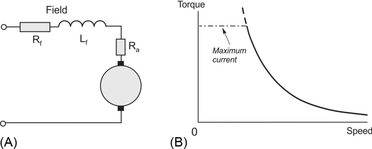
If the armature and field resistance volt-drops are neglected, and the applied voltage (V) is constant, the current varies inversely with the speed, hence the torque (T) and speed (n) are related by

A typical torque-speed characteristic is shown in Fig. 3.15B. The torque at zero speed is not infinite of course, because of the effects of saturation and resistance, both of which are ignored in Eq. (3.14).
As with the shunt motor, under starting conditions the back e.m.f. is zero, and if the full voltage was applied the current would be excessive, being limited only by the armature and field resistances. Hence for all but small motors a starting resistance is required to limit the current to a safe value.
Returning to Fig. 3.15B, we note that the series motor differs from most other motors in having no clearly defined no-load speed, i.e. no speed (other than infinity) at which the torque produced by the motor falls to zero. This means that when running light, the speed of the motor depends on the windage and friction torques, equilibrium being reached when the motor torque equals the total mechanical resisting torque. In large motors, the windage and friction torque is often relatively small, and the no-load speed is then too high for mechanical safety. Large series motors should therefore never be run uncoupled from their loads. As with shunt motors, the connections to either the field or armature must be reversed in order to reverse the direction of rotation.
The reason for the historic use of series motors for traction is that under the simplest possible supply arrangement (i.e. constant voltage) the overall shape of the torque-speed curve fits well with what is needed in traction applications, i.e. high starting torque to provide acceleration from rest and an acceptable reduction in acceleration as the target speed is approached. Early systems achieved coarse speed control via resistors switched in parallel with either the field or the armature in order to divert some of the current and thereby alter the torque-speed curve, but this inherently inefficient approach became obsolete when power electronic converters became available to provide an efficient variable-voltage supply.
3.7.3 Universal motors
In terms of numbers the main application area for the series commutator motor is in portable power tools, food mixers, vacuum cleaners, etc., where paradoxically the supply is a.c. rather than d.c. Such motors are often referred to as ‘universal’ motors because they can run from either a d.c. or an a.c. supply.
At first sight the fact that a d.c. machine will work on a.c. is hard to believe. But when we recall that in a series motor the field flux is set up by the current which also flows in the armature, it can be seen that reversal of the current will be accompanied by reversal of the direction of the magnetic flux, thereby ensuring that the torque remains positive. When the motor is connected to a 50 Hz supply for example, the (sinusoidal) current will change direction every 10 ms, and there will be a peak in the torque 100 times per second. But the torque will always remain unidirectional, and the speed fluctuations will not be noticeable because of the smoothing effect of the armature inertia.
Series motors for use on a.c. supplies are always designed with fully laminated construction (to limit eddy current losses produced by the pulsating flux in the magnetic circuit), and are intended to run at high speeds, say 8–12,000 rev/min. at rated voltage. Commutation and sparking are worse than when operating from d.c., and output powers are seldom greater than 1 kW. The advantage of high speed in terms of power output per unit volume was emphasised in Chapter 1, and the universal motor is a good example which demonstrates how a high power can be obtained with small size by designing for a high speed.
Until recently the universal motor offered the only relatively cheap way of reaping the benefit of high speed from single-phase a.c. supplies. Other small a.c. machines, such as induction motors and synchronous motors, were limited to maximum speeds of 3000 rev/min at 50 Hz (or 3600 rev/min at 60 Hz), and therefore could not compete in terms of power per unit volume. The availability of high-frequency inverters (see Chapter 7) has opened up the prospect of higher specific outputs from induction motors and PM motors in many appliances. The transition away from universal motor is underway, but because of the huge investment in high volume manufacturing that has been made over many years, they are still being produced in significant numbers.
Speed control of small universal motors is straightforward using a triac (in effect a pair of thyristors connected back to back) in series with the a.c. supply. By varying the firing angle, and hence the proportion of each cycle for which the triac conducts, the voltage applied to the motor can be varied to provide speed control. This approach is widely used for electric drills, fans etc. If torque control is required (as in hand power tools, for example), the current is controlled rather than the voltage, and the speed is determined by the load.
3.8 Self-excited d.c. machine
At various points in this chapter, we saw that the d.c. machine can change from motoring to generating depending on whether its induced or generated e.m.f. was less than or greater than the voltage applied to the armature terminals. We assumed that the machine was connected to a voltage source, from which it could draw both its excitation (field) and armature currents. But if we want to use the machine as a generator in a location isolated from any voltage source, we have to consider how to set up the flux to enable the machine to work as an energy converter.
When the field is provided by permanent magnets, there is no problem. As soon as the prime-mover (an internal combustion engine, perhaps) starts to turn the rotor, a speed-dependent e.m.f. (voltage) is produced in the armature and we can connect our load to the terminals and start to generate power. To ensure a more or less constant voltage, the engine will be governed to keep the speed constant.
If the machine has a field winding that is intended to be connected in parallel (shunt) with the armature, it is easy to imagine that once the machine is generating an armature voltage, there will be a field current and flux. But before we get a motional e.m.f. we need flux, and we can’t have flux without a field current, and we won’t get field current until we have generated an e.m.f.
The answer to this apparent difficulty usually lies in taking advantage of the residual magnetic flux remaining in the magnetic circuit from the time the machine was last used. If the residual flux is sufficient we will begin to generate as soon as the rotor is turned, and provided the field is connected the right way round across the armature, the first few milliamps of field current will increase the flux and we will then have positive feedback which we might expect to result in a runaway situation with ever-increasing generated voltage. Fortunately, provided that the driven speed is constant, the growth of flux is stabilised by saturation of the magnetic circuit, as we will discuss next. This procedure is known as self-excitation, for obvious reasons. (Should we be unfortunate enough to connect the field the wrong way round, we will be disappointed: but if the connections were undisturbed from the previous time, we should be OK.)
The stabilising effect of saturation is shown in Fig. 3.16. The solid line in the graph on the right is a typical ‘magnetisation curve’ of the machine. This is a plot of the generated e.m.f. (E) as a function of field current when the rotor is driven at a constant speed. This test is best done with a separate supply to the field, and (usually) at the rated speed. For low and medium values of the field current, the flux is proportional to the current, so the motional e.m.f. is linear, but at higher field currents the magnetic circuit starts to saturate, the flux no longer increases in proportion, and consequently the generated voltage flattens out. The armature circuit is open, so the terminal voltage (Va) is equal to the induced e.m.f. (E).
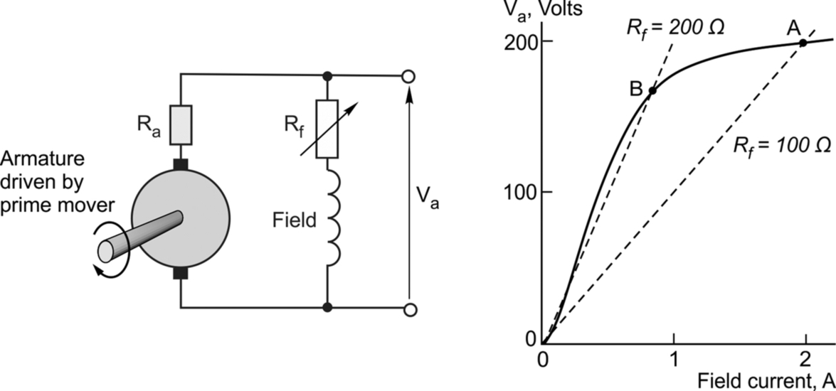
When we want the machine to self-excite, we connect the field in parallel with the armature as shown in Fig. 3.16. The current in the field is then given by If = Va/Rf where Rf is the resistance of the field winding, and we have neglected the small armature resistance. The two dotted lines relate to field circuit resistances of 100 and 200 Ω, and the intersection of these with the magnetisation curve give the stable operating points. For example, when the field resistance is 100 Ω, and the armature voltage is 200 V, the field current of 2 A is just sufficient to generate the motional e.m.f. of 200 V (point A). At lower values of field current, the generated voltage exceeds the value needed to maintain the field current, so the excess voltage cause the current to increase in the inductive circuit until the steady state is reached.
Increasing the resistance of the field circuit to 200 Ω results in a lower generated voltage (point B), but this is a less stable situation, with small changes in resistance leading to large changes in voltage. It should also be clear that if the resistance is increased above 200 Ω, the resistance line will be above the magnetisation curve, and self-excitation will be impossible.
3.9 Toy motors
The motors used in model cars, trains etc. are rather different in construction from those discussed so far, primarily because they are designed almost entirely with cost as the primary consideration. They also run at high speeds, so it is not important for the torque to be smooth. A typical arrangement used for rotor diameters from 0.5 cm to perhaps 3 cm is shown in Fig. 3.17.
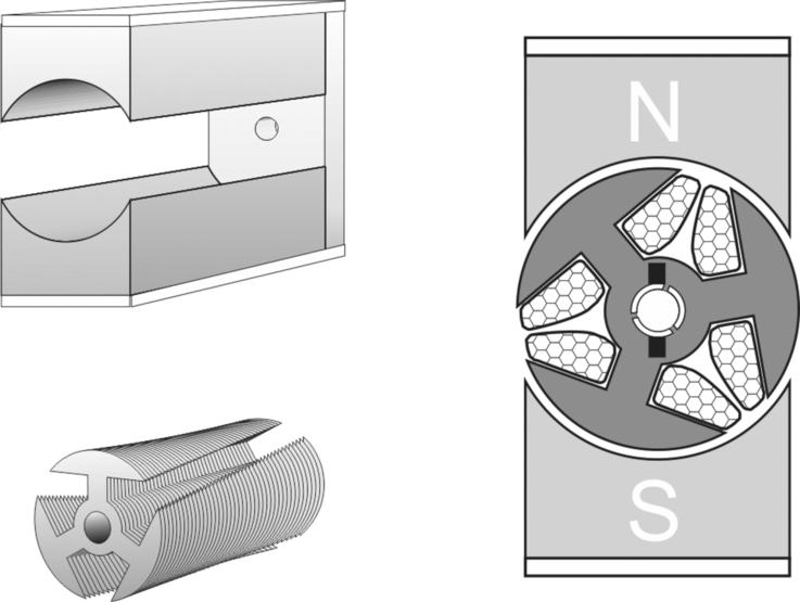
The rotor, made from laminations with a small number (typically three or five) of multi-turn coils in very large ‘slots,’ is simple to manufacture, and because the commutator has few segments, it too is cheap to make. The field system (stator) consists of radially-magnetised ceramic magnets with a steel backplate to complete the magnetic circuit.
The rotor clearly has very pronounced saliency, with three very large projections which are in marked contrast to the rotors we looked at earlier where the surface was basically cylindrical. It is easy to imagine that even when there is no current in the rotor coils, there is a strong tendency for the stator magnets to pull one or other of the rotor saliencies into alignment with a stator pole, so that the rotor would tend to lock in any one of six positions. This cyclic ‘detent’ torque, is due to the variation of reluctance with rotor position, an effect which is exploited in a.c. reluctance motors (see Chapter 9), but is unwanted here. To combat the problem the rotor laminations are skewed before the coils are fitted, as shown in the lower sketch on the left.
Each of the three rotor poles carries a multi-turn coil, the start of which is connected to a commutator segment, as shown in the cross-section on the right of Fig. 3.17. The three ends are joined together. The brushes are wider than the inter-segment space, so in some rotor positions the current from say the positive brush will divide and flow first through two coils in parallel until it reaches the common point, then through the third coil to the negative brush, while in other positions the current flows through only two coils.
A real stretch of imagination is required to picture the mechanism of torque production using the ‘BIl’ approach we have followed previously, as the geometry is so different. But we can take a more intuitive approach by considering, for each position, the polarity and strength of the magnetisation of each of the three rotor poles, which depend of course on the direction and magnitude of the respective currents. Following the discussion in the previous paragraph, we can see that in some positions there will be say a strong N and two relatively weak S poles, while at others there will be one strong N, one strong S, and one unexcited pole.
Thus although the rotor appears to be a three-pole device, the magnetisation pattern is always two-pole (because two adjacent weak S poles function as a single stronger S pole). When the rotor is rotating, the stator N pole will attract the nearest rotor S pole, pulling it round towards alignment. As the force of attraction diminishes to zero, the commutator reverses the rotor current in that pole so that it now becomes a N and is pushed away towards the S stator pole.
There is a variation of current with angular position as a result of the different resistances seen by the brushes as they alternately make contact with either one or two segments, and the torque is far from uniform, but operating speeds are typically several thousand rev/min and the torque pulsations are smoothed out by the rotor and load inertia.
3.10 Review questions
- (1)
- (a) What is the primary (external) parameter that determines the speed of an unloaded d.c. motor?
- (b) What is the primary external factor that determines the steady-state running current of a d.c. motor, for any given armature voltage?
- (c) What determines the small current drawn by a d.c. motor when running without any applied mechanical load?
- (d) What determines how much the speed of a d.c. motor reduces when the load on its shaft is increased? Why do little motors slow down more than large ones?
- (2) What has to be done to reverse the direction of rotation of:- (a) a separately-excited motor; (b) a shunt motor; (c) a series motor?
- (3) Most d.c. motors can produce much more than their continuously-rated torque. Why is it necessary to limit the continuous torque?
- (4) Why do d.c. motors run faster when their field flux is reduced?
- (5) A separately-excited d.c. motor runs from a 220 V d.c. supply and draws an armature current of 15 A. The armature resistance is 0.8 Ω. Calculate the generated voltage (back e.m.f).
If the field current is suddenly reduced by 10%, calculate (a) the value to which the armature current rises momentarily, and (b) the percentage increase in torque when the current reaches the value in (a). Ignore armature inductance, neglect saturation, and assume that the field flux is directly proportional to the field current. - (6)
- (a) When driven at 1500 rev/min the open-circuit armature voltage of a d.c. machine is 110 V. Calculate the e.m.f. constant in volts per radian/s. Calculate also the machine torque when the armature current is 10 A.
- (b) Suppose the machine was at rest, and a weight of 5 kg was suspended from a horizontal bar of length 80 cm attached to the shaft, as shown in Fig. Q6.

Fig. Q6
What current must be applied to the armature to keep the arm horizontal? Will the equilibrium be a stable one? (Neglect the mass of the bar; g = 9.81 m/s2.) - (c) When the machine runs as a motor drawing 25 A from a 110 V supply, the speed is 1430 rev/min. Calculate the armature resistance. Hence find the voltage needed to keep the bar in (b) horizontal.
- (d) At what speed must the machine be driven to supply 3.5 kW to a 110 V system?
Calculate the corresponding torque. If the field circuit consumes 100 W and the friction losses are 200 W, calculate the efficiency of the generator.
- (7) The equations expressing torque in terms of current (T = k I) and motional e.m.f. in terms of speed (E = k ω) are central in understanding the operation of a d.c. machine. Using only these equations, show that the mechanical output power is given by W = EI.
- (8) Explain briefly why:-
- (a) large d.c. motors cannot normally be started by applying full voltage;
- (b) the no-load speed of a permanent-magnet motor is almost proportional to the armature voltage.
- (c) a d.c. motor draws more current from the supply when the load on the shaft is increased.
- (d) the field windings of a d.c. motor consume energy continuously even though they do not contribute to the mechanical output power.
- (e) the field poles of a d.c. machine are not always laminated.
- (9) It is claimed in this book that a motor of a given size and power can be made available for operation at any voltage. But it is clear that, when it comes to battery-powered hand tools of a given size and speed, the higher-voltage versions are more powerful. What accounts for this contradiction?
- (10) This question relates to a permanent-magnet d.c. machine with an armature resistance of 0.5 Ω.
When the rotor is driven at 1500 rev/min by an external mechanical source, its open-circuit armature voltage is 220 V. All parts of the question relate to steady-state conditions, i.e. after all transients have died away.
The machine is to be used as a generator and act as a dynamic brake to restrain a lowering load, as shown in Fig. Q10A. The hanging mass of 14.27 kg is suspended by a rope from a 20 cm diameter winding drum on the motor shaft.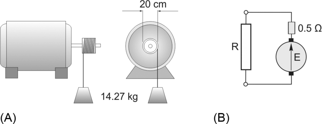
Fig. Q10
The majority of the generated power is to be dissipated in an external resistor (R) connected across the armature, as shown in Fig. Q10B.- (a) Calculate the value of resistance required so that the mass descends at a steady speed of 15 m/s. Take g = 9.81 m/s2.
- (b) What is the power dissipated in (i) the external resistor, (ii) the armature? Where does the energy dissipated in the resistors come from?
Answers to the review questions are given in the Appendix.