4.2.1 Motor operation with converter supply

The basic operation of the rectifying bridge has been discussed in Chapter 2, and we now turn to the matter of how the d.c. motor behaves when supplied with ‘d.c.’ from a controlled rectifier.

By no stretch of the imagination could the waveforms of armature voltage looked at in Chapter 2 (e.g. Fig. 2.13) be thought of as good d.c., and it would not be unreasonable to question the wisdom of feeding such an unpleasant-looking waveform to a d.c. motor. In fact it turns out that the motor works almost as well as it would if fed with pure d.c., for two main reasons. Firstly, the armature inductance of the motor causes the waveform of armature current to be much smoother than the waveform of armature voltage, which in turn means that the torque ripple is much less than might have been feared. And secondly, the inertia of the armature (and load) is sufficiently large for the speed to remain almost steady despite the torque ripple. It is indeed fortunate that such a simple arrangement works so well, because any attempt to smooth-out the voltage waveform (perhaps by adding smoothing capacitors) would prove to be prohibitively expensive in the power ranges of interest.

4.2.2 Motor current waveforms

For the sake of simplicity we will look at operation from a single-phase (two-pulse) converter, but similar conclusions apply to the six-pulse one. The voltage (V_a) applied to the motor armature is typically as shown in Fig. 4.3A: as we saw in Chapter 2, it consists of rectified ‘chunks’ of the incoming utility supply voltage, the precise shape and average value depending on the firing angle.

The voltage waveform can be considered to consist of a mean d.c. level (V_dc), and a superimposed pulsating or ripple component which we can denote loosely as v_ac. If the supply is at 50 Hz, the fundamental frequency of the ripple is 100 Hz. The mean voltage V_dc can be altered by varying the firing angle, which also incidentally alters the ripple (i.e. v_ac).

The ripple voltage causes a ripple current to flow in the armature, but because of the armature inductance, the amplitude of the ripple current is small. In other words, the armature presents a high impedance to a.c. voltages. This smoothing effect of the armature inductance is shown in Fig. 4.3B, from which it can be seen that the current ripple is relatively small in comparison with the corresponding voltage ripple. The average value of the ripple current is of course zero, so it has no effect on the average torque of the motor. There is nevertheless a variation in torque every half-cycle of the mains, but because it is of small amplitude and high frequency (100 or 120 Hz for the 1-phase case here, but 300 or 360 Hz for 3-phase, (both for 50 or 60 Hz supplies respectively)) the variation in speed (and hence back e.m.f., E) will not usually be noticeable.

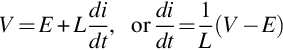
The current at the end of each pulse is the same as at the beginning, so it follows that the average voltage across the armature inductance (L) is zero. We can therefore equate the average applied voltage to the sum of the back e.m.f. (assumed pure d.c. because we are ignoring speed fluctuations) and the average voltage across the armature resistance, to yield

$V_{\mathit{dc}}=E+I_{\mathit{dc}}R$

which is exactly the same as for operation from a pure d.c. supply. This is very important, as it underlines the fact that we can control the mean motor voltage, and hence the speed, simply by varying the converter delay angle.

The smoothing effect of the armature inductance is important in achieving successful motor operation: the armature acts as a low-pass filter, blocking most of the ripple, and leading to a more or less constant armature current. For the smoothing to be effective, the armature time-constant needs to be long compared with the pulse duration (half a cycle with a two-pulse drive, but only one sixth of a cycle in a six-pulse drive). This condition is met in all almost all six-pulse drives, and in many two-pulse ones. Overall, the motor then behaves much as it would if it was supplied from an ideal d.c. source (though the I²R loss is higher than it would be if the current was perfectly smooth).

The no-load speed is determined by the applied voltage (which depends on the firing angle of the converter); there is a small drop in speed with load; and, as we have previously noted, the average current is determined by the load. In Fig. 4.3, for example, the voltage waveform in (A) applies equally for the two load conditions represented in (B), where the upper current waveform corresponds to a high value of load torque while the lower is for a much lighter load, the speed being almost the same in both cases. (The small difference in speed is due to the IR term, as explained in Chapter 3.) We should note that the current ripple remains the same—only the average current changes with load. Broadly speaking, therefore, we can say that the speed is determined by the converter firing angle, which represents a very satisfactory state of affairs because we can control the firing angle by low-power control circuits and thereby regulate the speed of the drive.

The current waveforms in Fig. 4.3B are referred to as ‘continuous’, because there is never any time during which the current is not flowing. This ‘continuous current’ condition is the norm in most drives, and it is highly desirable because it is only under continuous current conditions that the average voltage from the converter is determined solely by the firing angle, and is independent of the load current. We can see why this is so with the aid of Fig. 2.8, imagining that the motor is connected to the output terminals and that it is drawing a continuous current. For half of a complete cycle, the current will flow into the motor from T1 and return to the supply via T4, so the armature is effectively switched across the supply and the armature voltage is equal to the supply voltage, which is assumed to be ideal, i.e. it is independent of the current drawn. For the other half of the time, the motor current flows from T2 and returns to the supply via T3, so the motor is again hooked-up to the supply, but this time the connections are reversed. Hence the average armature voltage—and hence to a first approximation the speed—are defined once the firing angle is set.

4.2.3 Discontinuous current

We can see from Fig. 4.3B that as the load torque is reduced, there will come a point where the minima of the current ripple touch the zero-current line, i.e. the current reaches the boundary between continuous and discontinuous current. The load at which this occurs will also depend on the armature inductance, because the higher the inductance the smoother the current (i.e. the less the ripple). Discontinuous current mode is therefore most likely to be encountered in small machines with low inductance (particularly when fed from two-pulse converters) and under light-load or no-load conditions.

Typical armature voltage and current waveforms in the discontinuous mode are shown in Fig. 4.4, the armature current consisting of discrete pulses of current that occur only while the armature is connected to the supply, with zero current for the period (represented by θ in Fig. 4.3) when none of the thyristors are conducting and the motor is coasting free from the supply.

The shape of the current waveform can be understood by noting that with resistance neglected, Eq. 3.7 can be rearranged as

$\frac{\mathit{di}}{\mathit{dt}}=\frac{1}{L}\left(V-E\right)$

which shows that the rate of change of current (i.e. the gradient of the lower graph in Fig. 4.4) is determined by the instantaneous difference between the applied voltage V and the motional e.m.f. E. Values of (V–E) are shown by the vertical hatchings in Fig. 4.4, from which it can be seen that if V > E, the current is increasing, while if V < E, the current is falling. The peak current is thus determined by the area of the upper or lower shaded areas of the upper graph.

The firing angle in Figs. 4.3 and 4.4 is the same, at 60 degrees, but the load is less in Fig. 4.4 and hence the average current is lower (though, for the sake of the explanation offered below, the current axis in Fig. 4.4 is expanded as compared with that in Fig. 4.2). It should be clear by comparing these figures that the armature voltage waveforms (solid lines) differ because, in Fig. 4.4, the current falls to zero before the next firing pulse arrives and during the period shown as θ the motor floats free, its terminal voltage during this time being simply the motional e.m.f. (E). To simplify Fig. 4.4 it has been assumed that the armature resistance is small and that the corresponding volt-drop (I_aR_a) can be ignored. In this case, the average armature voltage (V_dc) must be equal to the motional e.m.f., because there can be no average voltage across the armature inductance when there is no net change in the current over one pulse: the hatched areas—representing the volt-seconds in the inductor—are therefore equal.

The most important difference between Figs. 4.3 and 4.4 is that the average voltage is higher when the current is discontinuous, and hence the speed corresponding to the conditions in Fig. 4.4 is higher than in Fig. 4.3 despite both having the same firing angle. And whereas in continuous mode a load increase can be met by an increased armature current without affecting the voltage (and hence speed), the situation is very different when the current is discontinuous. In the latter case, the only way that the average current can increase is for the speed (and hence E) to fall so that the shaded areas in Fig. 4.4 become larger.

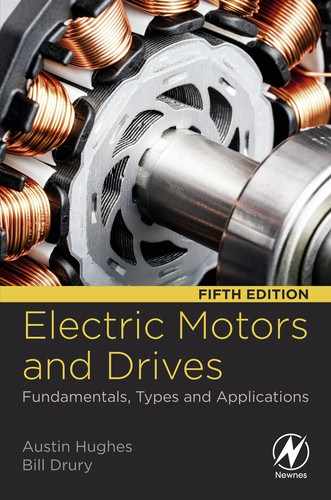
This means that the behaviour of the motor in discontinuous mode is much worse than in the continuous current mode, because as the load torque is increased, there is a serious drop in speed. The resulting torque-speed curve therefore has a very unwelcome ‘droopy’ characteristic in the discontinuous current region, as shown in Fig. 4.5, and in addition the I²R loss is much higher than it would be with pure d.c.

Under very light or no-load conditions, the pulses of current become virtually non-existent, the shaded areas in Fig. 4.4 become very small and the motor speed approaches that at which the back e.m.f. is equal to the peak of the supply voltage (point (C) in Fig. 4.5).

It is easy to see that inherent torque-speed curves with sudden discontinuities of the form shown in Fig. 4.5 are very undesirable. If, for example, the firing angle is set to zero and the motor is fully loaded, its speed will settle at point A, its average armature voltage and current having their full (rated) values. As the load is reduced, current remaining continuous, there is the expected slight rise in speed, until point B is reached. This is the point at which the current is about to enter the discontinuous phase. Any further reduction in the load torque then produces a wholly disproportionate—not to say frightening—increase in speed, especially if the load is reduced to zero, when the speed reaches point C.

There are two ways by which we can improve these inherently poor characteristics. Firstly, we can add extra inductance in series with the armature to further smooth the current waveform and lessen the likelihood of discontinuous current. The effect of adding inductance is shown by the dotted lines in Fig. 4.5. Secondly, we can switch from a single-phase converter to a three-phase one which produces smoother voltage and current waveforms, as discussed in Chapter 2.

When the converter and motor are incorporated in a closed-loop drive system the user should be unaware of any shortcomings in the inherent motor/converter characteristics because the control system automatically alters the firing angle to achieve the target speed at all loads. In relation to Fig. 4.5, for example, as far as the user is concerned the control system will confine operation to the shaded region, and the fact that the motor is theoretically capable of running unloaded at the high speed corresponding to point C is only of academic interest.

It is worth mentioning that discontinuous current operation is not restricted to the thyristor converter, but occurs in many other types of power electronic system. Broadly speaking, converter operation is more easily understood and analysed when in continuous current mode, and the operating characteristics are more desirable, as we have seen here. We will not dwell on the discontinuous mode in the rest of the book, as it is beyond our scope, and unlikely to be of concern to the drive user.

4.2.4 Converter output impedance: Overlap

So far we have tacitly assumed that the output voltage from the converter was independent of the current drawn by the motor, and depended only on the delay angle α. In other words we have treated the converter as an ideal voltage source.

In practice the a.c. supply has a finite impedance, and we must therefore expect a volt-drop which depends on the current being drawn by the motor. Perhaps surprisingly, the supply impedance (which is mainly due to inductive leakage reactances in transformers) manifests itself at the output stage of the converter as a supply resistance, so the supply volt-drop (or regulation) is directly proportional to the motor armature current.

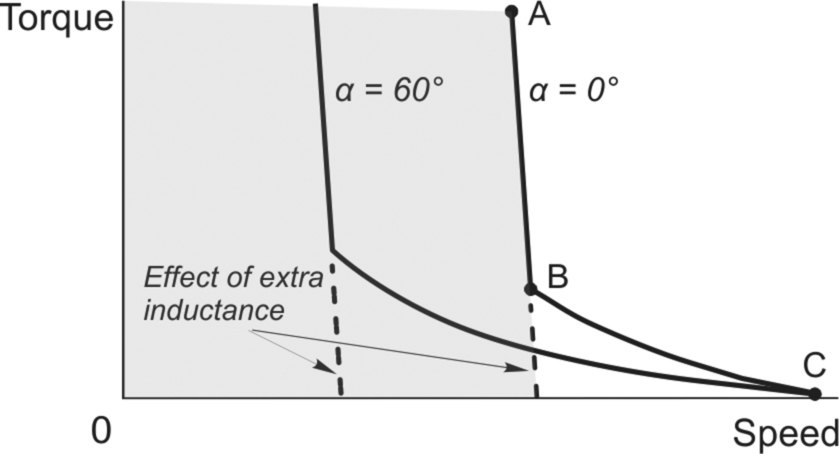
It is not appropriate to go into more detail here, but we should note that the effect of the inductive reactance of the supply is to delay the transfer (or commutation) of the current between thyristors, a phenomenon known as overlap. The consequence of overlap is that instead of the output voltage making an abrupt jump at the start of each pulse, there is a short period where two thyristors are conducting simultaneously. (The reader should not be alarmed at the mention of two devices conducting at the same time: they are not in the same arm, so there is not a short circuit path across the d.c. that we warned of in Chapter 2 when discussing the d.c. to a.c. inverter.) During this interval the output voltage is the mean of the voltages of the incoming and outgoing voltages, as shown typically in Fig. 4.6. When the drive is connected to a ‘stiff’ (i.e. low impedance) industrial supply the overlap will only last for perhaps a few microseconds, so the ‘notch’ shown in Fig. 4.6 would be barely visible on an oscilloscope. Books always exaggerate the width of the overlap for the sake of clarity, as in Fig. 4.6: with a 50 or 60 Hz supply, if the overlap lasts for more than say 1 ms, the implication is that the supply system impedance is too high for the size of converter in question, or conversely, the converter is too big for the supply.

Returning to the practical consequences of supply impedance, we simply have to allow for the presence of an extra ‘source resistance’ in series with the output voltage of the converter. This source resistance is in series with the motor armature resistance, and hence the motor torque-speed curves for each value of α have a somewhat steeper droop than they would if the supply impedance was zero. However, as part of a closed loop control system, the drive would automatically compensate for any speed droop resulting from overlap.

4.2.5 Four-quadrant operation and inversion

So far we have looked at the converter as a rectifier, supplying power from the a.c. utility supply to a d.c. machine running in the positive direction and acting as a motor. As explained in Chapter 3, this is known as 1-quadrant operation, by reference to quadrant 1 of the complete torque-speed plane shown in Fig. 3.12.

But suppose we want to run as a motor in the opposite direction, with negative speed and negative torque, i.e. in quadrant 3. How do we do it? And what about operating the machine as a generator, so that power is returned to the a.c. supply, the converter then ‘inverting’ power rather than rectifying, and the system operating in quadrant 2 or quadrant 4. We need to do this if we want to achieve regenerative braking. Is it possible, and if so how?

The good news is that as we saw in Chapter 3 the d.c. machine is inherently a bi-directional energy converter. If we apply a positive voltage V greater than E, a current flows into the armature and the machine runs as a motor. If we reduce V so that it is less than E, the current, torque and power automatically reverse direction, and the machine acts as a generator, converting mechanical energy (its own kinetic energy in the case of regenerative braking) into electrical energy. And if we want to motor or generate with the reverse direction of rotation, all we have to do is to reverse the polarity of the armature supply. The d.c. machine is inherently a four-quadrant device, but needs a supply which can provide positive or negative voltage, and simultaneously handle either positive or negative current.

This is where we meet a snag: a single thyristor converter can only handle current in one direction, because the thyristors are unidirectional devices. This does not mean that the converter is incapable of returning power to the supply however. The d.c. current can only be positive, but (provided it is a fully-controlled converter) the d.c. output voltage can be either positive or negative (see Chapter 2). The power flow can therefore be positive (rectification) or negative (inversion).

For normal motoring where the output voltage is positive (and assuming a fully-controlled converter), the delay angle (α) will be up to 90 degrees. (It is common practice for the firing angle corresponding to rated d.c. voltage to be around 20 degrees when the incoming a.c. voltage is normal: then if the a.c. voltage falls for any reason, the firing angle can be further reduced to compensate and still allow full “rated” d.c. voltage to be maintained.)

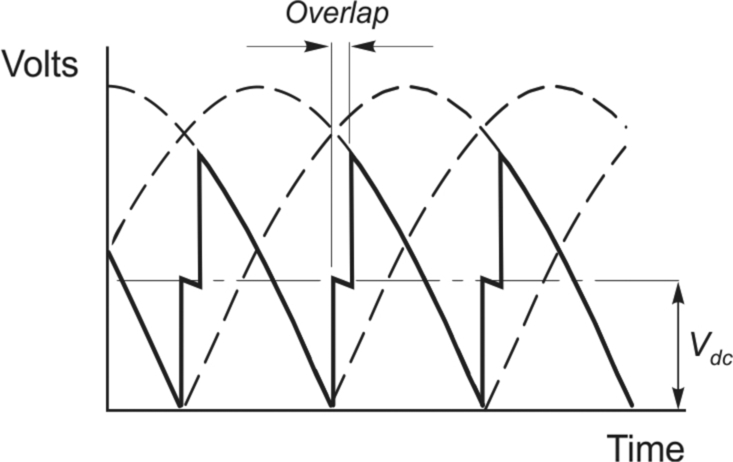
When α is greater than 90 degrees, however, the average d.c. output voltage is negative, as indicated by Eq. (2.5), and shown in Fig. 4.7. A single fully-controlled converter therefore has the potential for two-quadrant operation, though it has to be admitted that this capability is not easily exploited unless we are prepared to employ reversing switches in the armature or field circuits. This is discussed next.

4.2.6 Single-converter reversing drives

We will consider a fully-controlled converter supplying a permanent-magnet motor, and see how the motor can be regeneratively braked from full speed in one direction, and then accelerated up to full speed in reverse. We looked at this procedure in principle at the end of Chapter 3, but here we explore the practicalities of achieving it with a converter-fed drive. We should be clear from the outset that in practice, all the user has to do is to change the speed reference signal from full forward to full reverse: the control system in the drive converter takes care of matters from then on. What it does, and how, is discussed below.

When the motor is running at full speed forward, the converter delay angle will be small, and the converter output voltage V and current I will both be positive. This condition is shown in Fig. 4.8A, and corresponds to operation in quadrant 1.

In order to brake the motor, the torque has to be reversed. The only way this can be done is by reversing the direction of armature current. The converter can only supply positive current, however, so to reverse the motor torque we have to reverse the armature connections, using a mechanical switch or contactor, as shown in Fig. 4.8B. (Before operating the contactor, the armature current would be reduced to zero by lowering the converter voltage, so that the contactor is not required to interrupt current.) Note that because the motor is still rotating in the positive direction, the back e.m.f. remains in its original sense; but now the motional e.m.f. is seen to be assisting the current and so to keep the current within bounds the converter must produce a negative voltage V which is just a little less than E. This is achieved by setting the delay angle at the appropriate point between 90 and 180degrees. (The dotted line in Fig. 4.7 indicates that the maximum acceptable negative voltage will generally be somewhat less than the maximum positive voltage: this restriction arises because of the need to preserve a margin for commutation of current between thyristors.) Note that the converter current is still positive (i.e. upwards in Fig. 4.8B), but the converter voltage is negative, and power is thus flowing back to the supply system. In this condition the system is operating in quadrant 2, and the motor is decelerating because of the negative torque. As the speed falls, E reduces, and so V must be reduced progressively to keep the current at full value. This is achieved automatically by the action of the current-control loop, which is discussed later.

The current (i.e. torque) needs to be kept negative in order to run up to speed in the reverse direction, but after the back e.m.f. changes sign (as the motor reverses) the converter voltage again becomes positive and greater than E, as shown in Fig. 4.8C. The converter is then rectifying, with power being fed into the motor, and the system is operating in quadrant 3.

Schemes using reversing contactors are not suitable where the reversing time is critical or where periods of zero torque are unacceptable, because of the delay caused by the mechanical reversing switch, which may easily amount to 200–400 ms. Field reversal schemes operate in a similar way, but reverse the field current instead of the armature current. They are even slower, up to 5 s, because of the relatively long time-constant of the field winding.

4.2.7 Double-converter reversing drives

Where full four-quadrant operation and rapid reversal is called for, two converters connected in anti-parallel are used, as shown in Fig. 4.9. One converter supplies positive current to the motor, while the other supplies negative current.

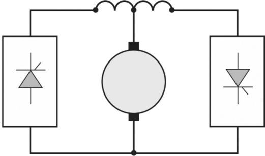
The bridges are operated so that their d.c. voltages are almost equal thereby ensuring that any d.c. circulating current is small—When the bridges are operated together in this way, a reactor is almost always placed between the bridges to limit the flow of ripple currents which result from the unequal instantaneous voltages of the two converters.

In most applications, the reactor can be dispensed with and the converters operated one at a time. The changeover from one converter to the other can only take place after the firing pulses have been removed from one converter, and the armature current has decayed to zero. Appropriate zero-current detection circuitry is provided as an integral part of the drive, so that as far as the user is concerned, the two converters behave as if they were a single ideal bi-directional d.c. source. There is a dead (torque-free) time typically of only 10 ms or so during the changeover period from one bridge to the other.

Prospective users need to be aware of the fact that a basic single converter can only provide for operation in one quadrant. If regenerative braking is required, either field or armature reversing contactors will be needed; and if rapid reversal is essential, a double converter has to be used. All these extras naturally push up the purchase price.

4.2.8 Power factor and supply effects

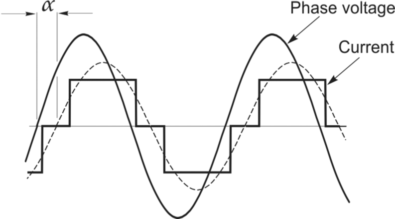
One of the drawbacks of a converter-fed d.c. drive is that the supply power-factor is very low when the motor is operating at low speed (i.e. low armature voltage), and is less than unity even at base speed and full load. This is because the supply current waveform lags the supply voltage waveform by the delay angle α, as shown (for a three-phase converter) in Fig. 4.10, and also the supply current is approximately rectangular (rather than sinusoidal).

It is important to emphasise that the supply power-factor is always lagging, even when the converter is inverting. There is no way of avoiding the low power-factor, so users of large drives need to be prepared to augment their existing power-factor correcting equipment if necessary.

The harmonics in the utility supply current waveform can give rise to a variety of disturbance problems, and supply authorities generally impose statutory limits. For large drives (say hundreds of kW), filters may have to be provided to prevent these limits from being exceeded.

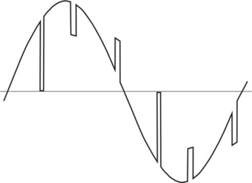
Since the supply impedance is never zero, there is also inevitably some distortion of the utility supply voltage waveform, as shown in Fig. 4.11, which indicates the effect of a six-pulse converter on the supply line-to-line voltage waveform. The spikes and notches arise because the utility supply is momentarily short-circuited each time the current commutates from one thyristor to the next, i.e. during the overlap period discussed earlier. For the majority of small and medium drives, connected to stiff industrial supplies, these notches are too small to be noticed (they are greatly exaggerated for the sake of clarity in Fig. 4.11); but they can cause serious disturbance to other consumers when a large drive is connected to a weak supply.

4.3.1 Current limits and protection

The closed-loop current controller, or current loop, is at the heart of the drive system and is indicated by the shaded region in Fig. 4.12. The purpose of the current loop is to make the actual motor current follow the current reference signal (I_ref) shown in Fig. 4.12. It does this by comparing a feedback signal of actual motor armature current with the current reference signal, amplifying the difference (the current error), and using the resulting current error signal to control the firing angle α—and hence the output voltage—of the converter. The current feedback signal is obtained either from a d.c. current transformer (which gives an isolated analogue voltage output), or from a.c. current transformer/rectifiers in the utility supply lines.

The job of comparing the reference (demand) and actual current signals and amplifying the error signal is carried out by the current-error amplifier. By giving the current-error amplifier a high gain, the actual motor current will always correspond closely to the current reference signal, i.e. the current-error will be small, regardless of motor speed. In other words, we can expect the actual motor current to follow the ‘current reference’ signal at all times, the armature voltage being automatically adjusted by the controller so that, regardless of the speed of the motor, the current has the correct value.

Of course no control system can be perfect, but it is usual for the current-error amplifier to be of the proportional plus integral (PI) type (see below), in which case the actual and demanded currents will be exactly equal under steady-state conditions.

The importance of preventing excessive converter currents from flowing has been emphasised previously, and the current control loop provides the means to this end. As long as the current control loop functions properly, the motor current can never exceed the reference value. Hence by limiting the magnitude of the current reference signal (by means of a clamping circuit), the motor current can never exceed the specified value. This is shown in Fig. 4.13, which represents a small portion of Fig. 4.12. The characteristics of the speed controller are shown in the shaded panel, from which we can see that for small errors in speed, the current reference increases in proportion to the speed error, thereby ensuring ‘linear system’ behaviour with a smooth approach to the target speed. However, once the speed error exceeds a limit, the output of the speed error amplifier saturates and there is thus no further increase in the current reference. By arranging for this maximum current reference to correspond to the full (rated) current of the system there is no possibility of the current in the motor and converter exceeding its rated value, no matter how large the speed error becomes.

This ‘electronic current limiting’ is by far the most important protective feature of any drive. It means that if for example the motor suddenly stalls because the load seizes (so that the back e.m.f. falls dramatically), the armature voltage will automatically reduce to a very low value, thereby limiting the current to its maximum allowable level.

The inner loop is critical in a two-loop control system, so the current loop must guarantee that the steady-state motor current corresponds exactly with the reference, and the transient response to step changes in the current reference should be fast and well damped. The first of these requirements is satisfied by the integral term in the current-error amplifier, while the second is obtained by judicious choice of the amplifier proportional gain and time-constant. As far as the user is concerned, a ‘current stability’ adjustment may be provided to allow him to optimise the transient response of the current loop.

On a point of jargon, it should perhaps be mentioned that the current-error amplifier is more often than not called either the ‘current controller’ (as in Fig. 4.12) or the ‘current amplifier’. The first of these terms is quite sensible, but the second can be very misleading: there is after all no question of the motor current itself being amplified.

4.3.2 Torque control

For applications requiring the motor to operate with a specified torque regardless of speed (e.g. in line tensioning), we can dispense with the outer (speed) loop, and simply feed a current reference signal directly to the current controller. This is because torque is directly proportional to current, so the current controller is in effect also a torque controller. We may have to make an allowance for accelerating torque, by means of a transient ‘inertia compensating’ signal, which could simply be added to the torque demand.

In the current-control mode the current remains constant at the set value, and the steady running speed is determined by the load. If the torque reference signal was set at 50%, for example, and the motor was initially at rest, it would accelerate with a constant current of half rated value until the load torque was equal to the motor torque. Of course, if the motor was running without any load, it would accelerate quickly, the applied voltage ramping up so that it always remained higher than the back e.m.f. by the amount needed to drive the specified current into the armature. Eventually the motor would reach a speed (a little above normal ‘full’ speed) at which the converter output voltage had reached its upper limit, and it was therefore no longer possible to maintain the set current: thereafter, the motor speed would remain steady.

This discussion assumes that torque is proportional to armature current, which is true only if the flux is held constant, which in turn requires the field current to be constant. Hence in all but small drives the field will be supplied from a thyristor converter with current feedback. Variations in field circuit resistance due to temperature changes, and/or changes in the utility supply voltage are thereby automatically compensated and the flux is maintained at its rated value.

4.3.3 Speed control

The outer loop in Fig. 4.12 provides speed control. Speed feedback is typically provided by a d.c. tacho, and the actual and required speeds are fed into the speed-error amplifier (often known simply as the speed amplifier or the speed controller).

Any difference between the actual and desired speed is amplified, and the output serves as the input to the current loop. Hence if for example the actual motor speed is less than the desired speed, the speed amplifier will demand current in proportion to the speed error, and the motor will therefore accelerate in an attempt to minimise the speed error.

When the load increases, there is an immediate deceleration and the speed error signal increases, thereby calling on the inner loop for more current. The increased torque results in acceleration and a progressive reduction of the speed error until equilibrium is reached at the point where the current reference (I_ref) produces a motor current that gives a torque equal and opposite to the load torque. Looking at Fig. 4.13, where the speed controller is shown as a simple proportional amplifier (P control), it will be readily appreciated that in order for there to be a steady-state value of I_ref, there would have to be a finite speed error, i.e. a P controller would not allow us to reach exactly the target speed. (We could approach the ideal by increasing the gain of the amplifier, but that might lead us to instability.)

To eliminate the steady-state speed error we can easily arrange for the speed controller to have an integral (I) term as well as a proportional (P) term. A PI controller can have a finite output even when the input is zero, which means that we can achieve zero steady-state error if we employ PI control.

The speed will be held at the value set by the speed reference signal for all loads up to the point where full armature current is needed. If the load torque increases any more the speed will drop because the current-loop will not allow any more armature current to flow. Conversely, if the load attempted to force the speed above the set value, the motor current will be reversed automatically, so that the motor acts as a brake and regenerates power to the utility supply.

To emphasise further the vitally important protective role of the inner loop, we can see what happens when, with the motor at rest (and unloaded for the sake of simplicity), we suddenly increase the speed reference from zero to full value, i.e. we apply a step demand for full speed. The speed error will be 100%, so the output from the speed-error amplifier (I_ref) will immediately saturate at its maximum value, which has been deliberately clamped so as to correspond to a demand for the maximum (rated) current in the motor. The motor current will therefore be at rated value, and the motor will accelerate at full torque. Speed and back e.m.f. (E) will therefore rise at a constant rate, the applied voltage (V) increasing steadily so that the difference (V–E) is sufficient to drive rated current (I) through the armature resistance. A very similar sequence of events was discussed in Chapter 3, and illustrated by the second half of Fig. 3.13. (In some drives the current reference is allowed to reach 150% or even 200% of rated value for a few seconds, in order to provide a short torque-boost. This is particularly valuable in starting loads with high static friction, and is known as a ‘two-stage current limit’).

The output of the speed amplifier will remain saturated until the actual speed is quite close to the target speed, and for all this time the motor current will therefore be held at full value. Only when the speed is within a few per cent of target will the speed error amplifier come out of saturation. Thereafter, as the speed continues to rise, and the speed error falls, the output of the speed error amplifier falls below the clamped level. Speed control then enters a linear regime, in which the correcting current (and hence the torque) is proportional to speed error, giving a smooth approach to final speed.

A ‘good’ speed controller will result in zero steady-state error, and have a well-damped response to step changes in the demanded speed. The integral term in the PI control caters for the requirement of zero steady-state error, while the transient response depends on the setting of the proportional gain and time-constant. The ‘speed stability’ setting (traditionally a potentiometer) is provided to allow fine tuning of the transient response. It should be mentioned that in some high-performance drives the controller will be of the PID form, i.e. it will also include a differential (D) term. The D term gives a bit of a kick to the controllers when a step change is called for—in effect advanced warning that we need a bit of smart action to change the current in the inductive circuit.

It is important to remember that it is much easier to obtain a good transient response with a regenerative drive, which has the ability to supply negative current (i.e. braking torque) should the motor overshoot the desired speed. A non-regenerative drive cannot furnish negative current (unless fitted with reversing contactors), so if the speed overshoots the target the best that can be done is to reduce the armature current to zero and wait for the motor to decelerate naturally. This is not satisfactory, and every effort therefore has to be made to avoid controller settings which lead to an overshoot of the target speed.

As with any closed-loop scheme, problems occur if the feedback signal is lost when the system is in operation. If the tacho feedback became disconnected, the speed amplifier would immediately saturate, causing full torque to be applied. The speed would then rise until the converter output reached its maximum output voltage. To guard against this many drives incorporate tacho-loss detection circuitry, and in some cases armature voltage feedback (see later section) automatically takes over in the event of tacho failure.

Drives which use field-weakening to extend the speed range include automatic provision for controlling both armature voltage and field current when running above base speed. Typically, the field current is kept at full value until the armature voltage reaches about 95% of rated value. When a higher speed is demanded, the extra armature voltage applied is accompanied by a simultaneous reduction in the field current, in such a way that when the armature voltage reaches 100% the field current is at the minimum safe value.

4.3.4 Overall operating region

A standard drive with field-weakening provides armature voltage control of speed up to base speed, and field-weakening control of speed thereafter. Any torque up to the rated value can be obtained at any speed below base speed, and as explained in Chapter 3 this region is known as the ‘constant torque’ region. Above base speed, the maximum available torque reduces inversely with speed, so this is known as the ‘constant power’ region. For a converter-fed drive the operating region in quadrant 1 of the torque-speed plane is therefore as shown in Fig. 3.10. (If the drive is equipped for regenerative and reversing operation, the operating area is mirrored in the other three quadrants, of course.)

4.3.5 Armature voltage feedback and IR compensation

In low-power drives where precision speed-holding is not essential, and cost must be kept to a minimum, the tacho may be dispensed with and the armature voltage used as a ‘speed feedback’ instead. Performance is clearly not as good as with tacho feedback, since whilst the steady-state no-load speed is proportional to armature voltage, the speed falls as the load (and hence armature current) increases.

We saw in Chapter 3 that the drop in speed with load was attributable to the armature resistance volt-drop (IR), and the steady-state drop in speed can therefore be compensated by boosting the applied voltage in proportion to the current. ‘IR compensation’ would in such cases be provided on the drive circuit for the user to adjust to suit the particular motor. The compensation is far from perfect, since it cannot cope well with temperature variation of resistance, nor with load transients.

4.3.6 Drives without current control

Very low cost, low power drives may dispense with a full current control loop, and incorporate a crude ‘current-limit’ which only operates when the maximum set current would otherwise be exceeded. These drives usually have an in-built ramp circuit which limits the rate of rise of the set speed signal so that under normal conditions the current limit is not activated. They are however prone to tripping in all but the most controlled of applications and environments.

4.4.1 Performance of chopper-fed d.c. motor drives

We saw earlier that the d.c. motor performed almost as well when fed from a phase-controlled rectifier as it does when supplied with pure d.c. The chopper-fed motor is, if anything, rather better than the phase-controlled, because the armature current ripple can be less if a high chopping frequency is used.

A typical circuit and waveforms of armature voltage and current are shown in Fig. 4.14: these are drawn with the assumption that the switch is ideal. The rather modest chopping frequency of 100 Hz shown in Fig. 4.14 has been deliberately chosen so that the current ripple is significant in relation to the average current (I_dc), and so that the relationship to the voltage waveform is clearly shown. In practice, most chopper drives operate at much higher frequencies, and the ripple current is therefore much less significant. As usual, we have assumed that the speed remains constant despite the slightly pulsating torque, and that the armature current is continuous.

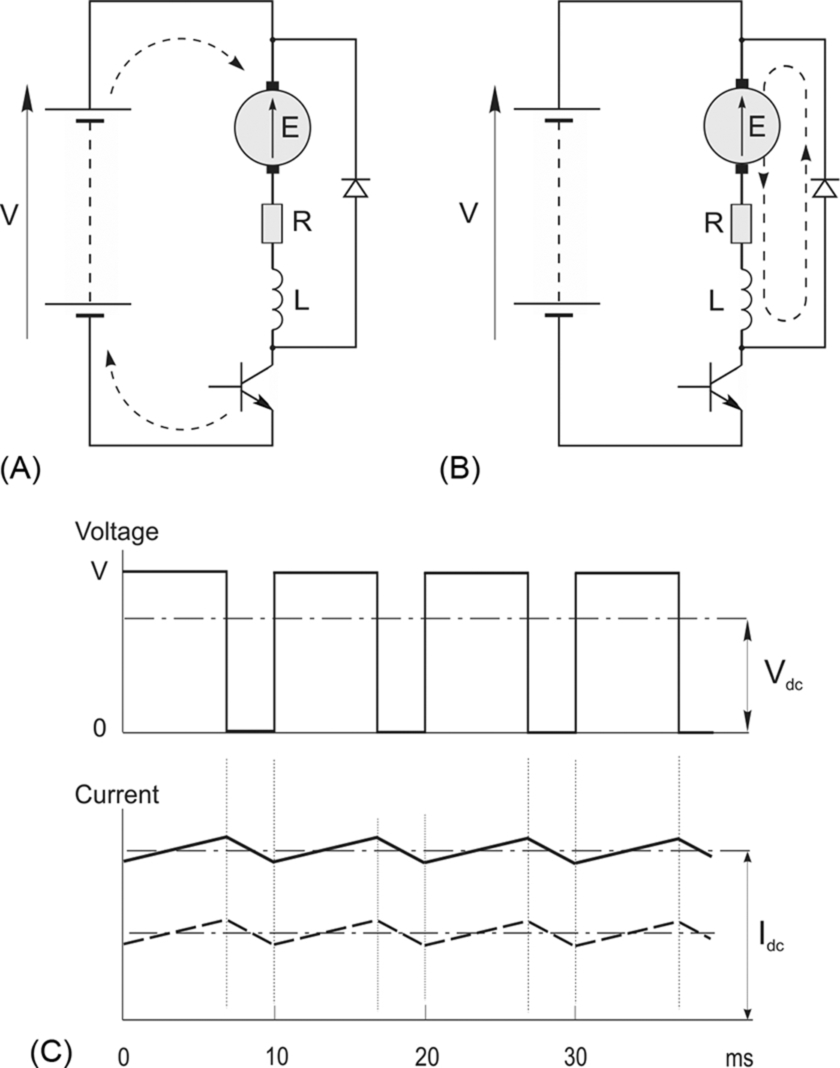
The shape of the armature voltage waveform reminds us that when the transistor is switched on, the battery voltage V is applied directly to the armature, and during this period the path of the armature current is indicated by the dotted line in Fig. 4.14A. For the remainder of the cycle the transistor is turned ‘off’ and the current freewheels through the diode, as shown by the dotted line in Fig. 4.14B. When the current is freewheeling through the diode, the armature voltage is clamped at (almost) zero.

The speed of the motor is determined by the average armature voltage, (V_dc), which in turn depends on the proportion of the total cycle time (T) for which the transistor is ‘on’. If the on and off times are defined as T_on = kT and T_off = (1 − kT), where 0 < k < 1, then the average voltage is simply given by

$V_{\mathit{dc}}=\mathit{kV}$

from which we see that speed control is effected via the on time ratio, k.

Turning now to the current waveforms shown in Fig. 4.14C, the upper waveform corresponds to full load, i.e. the average current (I_dc) produces the full rated torque of the motor. If now the load torque on the motor shaft is reduced to half rated torque, and assuming that the resistance is negligible, the steady-state speed will remain the same but the new mean steady-state current will be halved, as shown by the lower dotted curve. We note however that although, as expected, the mean current is determined by the load, the ripple current is unchanged, and this is explained below.

If we ignore resistance, the equation governing the current during the ‘on’ period is

$V=E+L\frac{\mathit{di}}{\mathit{dt}},\text{or}\frac{\mathit{di}}{\mathit{dt}}=\frac{1}{L}\left(V-E\right)$

Since V is greater than E, the gradient of the current (di/dt) is positive, as can be seen in Fig. 4.14C. During this ‘on’ period the battery is supplying power to the motor. Some of the energy is converted to mechanical output power, but some is also stored in the magnetic field associated with the inductance. The latter is given by $\frac{1}{2}L{i}^2$, and so as the current (i) rises, more energy is stored.

During the ‘off’ period, the equation governing the current is

$0=E+L\frac{di}{dt},\mathrm{or}\frac{di}{dt}=\frac{-E}{L}$

We note that during the ‘off’ time the gradient of the current is negative (as shown in Fig. 4.14C) and it is determined by the motional e.m.f. E. During this period, the motor is producing mechanical output power which is supplied from the energy stored in the inductance, so not surprisingly the current falls as the energy previously stored in the on period is now given up.

We note that the rise and fall of the current (i.e. the current ripple) is inversely proportional to the inductance, but is independent of the mean d.c. current, i.e. the ripple does not depend on the load.

To study the input/output power relationship, we note that the battery current only flows during the on period, and its average value is therefore kI_dc. Since the battery voltage is constant, the power supplied is simply given by V(kI_dc) = kVI_dc. Looking at the motor side, the average voltage is given by V_dc = kV, and the average current (assumed constant) is I_dc, so the power input to the motor is again kVI_dc i.e. there is no loss of power in the ideal chopper. Given that k is < 1, we see that the input (battery) voltage is higher than the output (motor) voltage, but conversely the input current is less than the output current, and in this respect we see that the chopper behaves in much the same way for d.c. as a conventional transformer does for a.c.

4.4.2 Torque-speed characteristics and control arrangements

Under open-loop conditions (i.e. where the mark-space ratio of the chopper is fixed at a particular value) the behaviour of the chopper-fed motor is similar to the converter-fed motor discussed earlier (see Fig. 4.4). When the armature current is continuous the speed falls only slightly with load, because the mean armature voltage remains constant. But when the armature current is discontinuous (which is most likely at high speeds and light load) the speed falls off rapidly when the load increases, because the mean armature voltage falls as the load increases. Discontinuous current can be avoided by adding an inductor in series with the armature, or by raising the chopping frequency, but when closed-loop speed control is employed, the undesirable effects of discontinuous current are masked by the control loop.

The control philosophy and arrangements for a chopper-fed motor are the same as for the converter-fed motor, with the obvious exception that the mark-space ratio of the chopper is used to vary the output voltage, rather than the firing angle.

4.5.1 Servo motors

Although there is no sharp dividing line between servo motors and ordinary motors, the servo type will usually be intended for use in applications which require rapid acceleration and deceleration. The design of the motor will reflect this by catering for intermittent currents (and hence torques) of many times the continuously rated value. Because most servo motors are small, their armature resistances are relatively high: the short-circuit (locked-rotor) current at full armature voltage is therefore perhaps only a few times the continuously rated current, and the drive amplifier will normally be selected so that it can cope with this condition, giving the motor a very rapid acceleration from rest. The even more arduous condition in which the full armature voltage is suddenly reversed with the motor running at full speed is also quite normal. (Both of these modes of operation would of course be quite unthinkable with a large d.c. motor, because of the huge currents which would flow as a result of the disproportionately low armature resistance.)

In order to maximise acceleration, the rotor inertia must be minimised, and one obvious way to achieve this is to construct a motor in which only the electric circuit (conductors) on the rotor move, the magnetic part (either iron or permanent magnet) remaining stationary. This principle is adopted in ‘ironless rotor’ and ‘printed armature’ motors.

In the ironless rotor or moving-coil type (Fig. 4.15) the armature conductors are formed as a thin-walled cylinder consisting essentially of nothing more than varnished wires wound in skewed form together with the disc-type commutator (not shown). Inside the armature sits a two-pole (upper N, lower S) permanent magnet which provides the radial flux, and outside it is a steel cylindrical shell which completes the magnetic circuit.

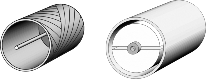
Needless to say the absence of any slots to support the armature winding results in a relatively fragile structure, which is therefore limited to diameters of not much over 1 cm. Because of their small size they are often known as micromotors, and are very widely used in cameras, video systems, card readers, medical instruments etc.

The printed armature type is altogether more robust, and is made in sizes up to a few kW. They are generally made in disc or pancake form, with the direction of flux axial and the armature current radial. The armature conductors resemble spokes on a wheel, the conductors themselves being formed on a lightweight disc. Early versions were made by using printed-circuit techniques, but pressed fabrication is now more common. Since there are usually at least a hundred armature conductors, the torque remains almost constant as the rotor turns, which allows them to produce very smooth rotation at low speed. Inertia and armature inductance are low, giving a good dynamic response, and the short and fat shape makes them suitable for applications such as machine tools and disc drives where axial space is at a premium.

It is worth briefly mentioning that there is another type of servo motor, where extremely smooth rotation is the primary consideration. Here, rotor inertia is usually maximised. Such an applications would be a machine tool spindle, where any variation in the rotational speed during a cutting process could be reflected in surface imperfections in the finished product.

4.5.2 Position control

As mentioned earlier, many servo motors are used in closed-loop position control applications, so it is appropriate to look briefly at how this is achieved. Later (in Chapter 10) we will see that the stepping motor provides an alternative open-loop method of position control, which can be cheaper for some less demanding applications.

In the example shown in Fig. 4.16, the angular position of the output shaft is intended to follow the reference voltage (θ_ref), but it should be clear that if the motor drives a toothed belt linear outputs can also be obtained. The potentiometer mounted on the output shaft provides a feedback voltage proportional to the actual position of the output shaft. The voltage from this potentiometer must be a linear function of angle, and must not vary with temperature, otherwise the accuracy of the system will be in doubt.

The feedback voltage (representing the actual angle of the shaft) is subtracted from the reference voltage (representing the desired position) and the resulting position error signal is amplified and used to drive the motor so as to rotate the output shaft in the desired direction. When the output shaft reaches the target position, the position error becomes zero, no voltage is applied to the motor, and the output shaft remains at rest. Any attempt to physically move the output shaft from its target position immediately creates a position error and a restoring torque is applied by the motor.

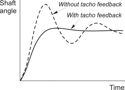
The dynamic performance of the simple scheme described above is very unsatisfactory as it stands. In order to achieve a fast response and to minimise position errors caused by static friction, the gain of the amplifier needs to be high, but this in turn leads to a highly oscillatory response which is usually unacceptable. For some fixed-load applications matters can be improved by adding a compensating network at the input to the amplifier, but the best solution is to use ‘tacho’ (speed) feedback (shown dotted in Fig. 4.16) in addition to the main position feedback loop. Tacho feedback clearly has no effect on the static behaviour (since the voltage from the tacho is proportional to the speed of the motor), but has the effect of increasing the damping of the transient response. The gain of the amplifier can therefore be made high in order to give a fast response, and the degree of tacho feedback can then be adjusted to provide the required damping (see Fig. 4.17). Many servo motors have an integral tacho for this purpose. (This is a particular example of the general principle by which the response can be improved by adding ‘derivative of output’ feedback: in this case the speed signal is the rate of change (or derivative) of the angular position.)

The example above dealt with an analogue scheme in the interests of simplicity, but digital position control schemes (with an encoder used to provide both position and speed information) are now much more common, especially when brushless motors (see Chapter 9) are used. Complete ‘controllers on a card’ are available as off-the-shelf items, and these offer ease of interface to other systems as well as providing for improved flexibility in shaping the dynamic response.