3. Rate Laws
Success is measured not so much by the position one has reached in life, as by the obstacles one has overcome while trying to succeed.
—Booker T. Washington
3.1 Basic Definitions
A homogeneous reaction is one that involves only one phase. A heterogeneous reaction involves more than one phase, and the reaction usually occurs at the interface between the phases. An irreversible reaction is one that proceeds in only one direction and continues in that direction until one of the reactants is exhausted. A reversible reaction, on the other hand, can proceed in either direction, depending on the temperature and on the concentrations of reactants and products relative to the corresponding equilibrium concentrations. An irreversible reaction behaves as if no equilibrium condition exists. Strictly speaking, no chemical reaction is completely irreversible. However, for many reactions, the equilibrium point lies so far to the product side that these reactions are treated as irreversible reactions.
Types of reactions
The molecularity of a reaction is the number of atoms, ions, or molecules involved (colliding) in a reaction step. The terms unimolecular, bimolecular, and termolecular refer to reactions involving, respectively, one, two, and three atoms (or molecules) interacting or colliding in any one reaction step. The most common example of a unimolecular reaction is radioactive decay, such as the spontaneous emission of an alpha particle from uranium-238 to give thorium and helium
92U238 → 90Th234 + 2He4
The rate of disappearance of uranium (U) is given by the rate law
–rU = kCU
The only true bimolecular reactions are those that involve the collision with free radicals (i.e., unpaired electrons, e.g., Br•), such as
Br• + C2H6 → HBr + C2H5•
with the rate of disappearance of bromine given by the rate law
–rBr• = kCBr•CC2H6
The probability of a termolecular reaction, where three molecules collide all at once, is almost nonexistent, and in most instances the reaction pathway follows a series of bimolecular reactions, as in the case of the reaction
2NO + O2 → 2NO2
The reaction pathway for this “Hall of Fame” reaction is quite interesting and is discussed in Problem P9-5A and also in Chapter 9 where similar reactions that form active intermediate complexes in their reaction pathways are given.
In discussing rates of chemical reactions, we have three rates to consider:
Relative Rates
Rate Laws
Net Rates
Relative rates tell us how fast one species is disappearing or appearing relative to the other species in the given reaction.
Rate laws are the algebraic equations that give the rate of reaction as a function of the reacting species concentrations and of temperature in a specific reaction.
Net rates of formation of a given species (e.g., A) is the sum of the rate of reactions of A in all the reactions in which A is either a reactant or product in the system.
A thorough discussion of net rates is given in Table 8-2 in Chapter 8, where we discuss multiple reactions.
3.1.1 Relative Rates of Reaction
The relative rates of reaction of the various species involved in a reaction can be obtained from the ratio of the stoichiometric coefficients.† For Reaction (2-2),
Reaction stoichiometry
we see that for every mole of A that is consumed, c/a moles of C appear. In other words,
Rate of formation of × (Rate of disappearance of A)
Similarly, the relationship between the rates of formation of C and D is
The relationship can be expressed directly from the stoichiometry of the reaction
for which
or
Useful Neumonics
For example, in the reaction
2NO + O2 ⇄ 2NO2
we have
If NO2 is being formed at a rate of 4 mol/m3/s, that is,
rNO2 = 4 mol/m3/s
†Tutorial Video: https://www.youtube.com/watch?v=wYqQCojggyM
then the rate of formation of NO is
the rate of disappearance of NO is
–rNO = 4 mol/m3/s
Summary
and the rate of disappearance of oxygen, O2, is
3.2 The Rate Law
To understand the rate of reaction, we need to describe three molecular concepts. In Concept 1: Law of Mass Action, we use rate laws to relate the rate of reaction to the concentrations of the reacting species. Concept 2: Potential Energy Surfaces and Concept 3: The Energy Needed for Crossing the Barriers help us explain the effect of temperature on the rate of reaction.
In the chemical reactions considered in the following paragraphs, we take as the basis of calculation a species A, which is one of the reactants that is disappearing as a result of the reaction. The limiting reactant is usually chosen as our basis for calculation. The rate of disappearance of A, –rA, depends on temperature and concentration. For many irreversible reactions, it can be written as the product of a reaction rate constant, kA, and a function of the concentrations (activities) of the various species involved in the reaction:
Concept 1: Law of Mass Action. The rate of reaction increases with increasing concentration of reactants which leads to a corresponding increase in the number of molecular collisions. The rate law for bimolecular collisions is derived in the collision theory section of the Professional Reference Shelf R3.1 (http://www.umich.edu/~elements/6e/03chap/prof.html). A schematic of the reaction of A and B molecules colliding and reacting is shown in Figure R3.1 on page 108.
The algebraic equation that relates the rate of reaction –rA to the species concentrations is called the kinetic expression or rate law.† The specific rate of reaction (also called the rate constant), kA, like the reaction rate, –rA, always refers to a particular species in the reaction and normally should be subscripted with respect to that species. However, for reactions in which the stoichiometric coefficient is 1 for all species involved in the reaction, for example,
1 NaOH + 1 HCl → 1 NaCl + 1 H2O
The rate law gives the relationship between reaction rate and concentration.
we shall delete the subscript on the specific reaction rate, (e.g., A in kA), to let
k = kNaOH = kHCl = kNaCl = kH2O
†Tutorial Video: https://www.youtube.com/watch?v=6mAqX31RRJU
3.2.1 Power Law Models and Elementary Rate Laws
The dependence of the reaction rate, –rA, on the concentrations of the species present, fn(Cj), is almost without exception determined by experimental observation. Although the functional dependence on concentration may be postulated from theory, experiments are necessary to confirm the proposed form. One of the most common general forms of this dependence is the power-law model. Here the rate law is the product of concentrations of the individual reacting species, each of which is raised to a power, for example,

The exponents of the concentrations in Equation (3-3) lead to the concept of reaction order. The order of a reaction refers to the powers to which the concentrations are raised in the kinetic rate law.† In Equation (3-3), the reaction is α order with respect to reactant A, and β order with respect to reactant B. The overall order of the reaction, n, is
n = α + β
Overall reaction order
The units of –rA are always in terms of concentration per unit time, while the units of the specific reaction rate, kA, will vary with the order of the reaction. Consider a reaction involving only one reactant, such as
A → Products
with an overall reaction order n. The units of rate, –rA, and the specific reaction rate, k are
{–rA } = [concentration/time]
and
Generally, the overall reaction order can be deduced from the units of the specific reaction-rate constant k. For example, the rate laws corresponding to a zero-, first-, second-, and third-order reaction, together with typical units for the corresponding rate constants, are
Zero-order (n = 0):
– rA = kA:
† Strictly speaking, the reaction rates should be written in terms of the activities, ai, (ai = γiCi, where γi is the activity coefficient). Kline and Fogler, JCIS, 82, 93 (1981); ibid., p. 103; and Ind. Eng. Chem Fundamentals 20, 155 (1981).
However, for many reacting systems, the activity coefficients, γi, do not change appreciably during the course of the reaction, and they are absorbed into the specific reaction-rate constant, kA
First order (n = 1):
Second order (n = 2):
Third order (n = 3):
An elementary reaction is one that involves a single reaction step, such as the bimolecular reaction between an oxygen free radical and methanol molecule:
O• + CH3OH → CH3O• + OH•
The stoichiometric coefficients in this reaction are identical to the powers in the rate law. Consequently, the rate law for the disappearance of molecular oxygen is
–rO• = kCO• CCH3OH
The reaction is first order in an oxygen free radical and first order in methanol; therefore, we say that both the reaction and the rate law are elementary. This form of the rate law can be derived from Collision Theory, as shown in the Professional Reference Shelf R3.1 on the CRE Web site (www.umich.edu/~elements/6e/index.html). There are many reactions where the stoichiometric coefficients in the reaction are identical to the reaction orders, but the reactions are not elementary, owing to such things as pathways involving active intermediates and series reactions. For these reactions that are not elementary but whose stoichiometric coefficients are identical to the reaction orders in the rate law, we say the reaction follows an elementary rate law. For example, the oxidation reaction of nitric oxide discussed earlier
2NO + O2 → 2NO2

Collision theory
is not really an elementary reaction, but follows an elementary rate law, that is, second order in NO and first order in O2, therefore,
Note: The rate constant, k, is defined with respect to NO.
Another nonelementary reaction that follows an elementary rate law is the gas-phase reaction between hydrogen and iodine
H2 + I2 → 2HI
and is first order in H2 and first order in I2, with
→rH2 = kH2CH2CI2
In summary, for many reactions involving multiple steps and pathways, the powers in the rate laws surprisingly agree with the stoichiometric coefficients. Consequently, to facilitate describing this class of reactions, we say that a reaction follows an elementary rate law when the reaction orders are identical to the stoichiometric coefficients of the reacting species for the reaction as written. It is important to remember that the rate laws are determined by experimental observation! Chapter 7 describes how these and other rate laws can be developed from experimental data. They are a function of the reaction chemistry and not the type of reactor in which the reactions occur. Table 3-1 gives examples of rate laws for a number of reactions. By saying a reaction follows an elementary rate law as written gives us a quick way to look at the reaction stoichiometry and then write the mathematical form of the rate law. The values of specific reaction rates for these and a number of other reactions can be found in the Database found in the footnote below.
TABLE 3-1 EXAMPLES OF REACTION-RATE LAWS
A. First-Order Rate Laws
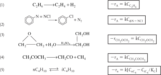
B. Second-Order Rate Laws
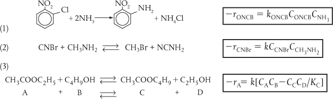
C. Nonelementary Rate Laws
(1) Homogeneous
(2) Heterogeneous

D. Enzymatic Reactions (Urea (U) + Urease (E))
NH2CONH2 + Urease + H2O → 2NH3 + CO2 + Urease
E. Biomass Reactions
Substrate (S) + Cells (C) → More Cells + Product
Note: The rate constants, k, and activation energies for a number of the reactions in these examples are given in the Databases in Appendix E. For more rate laws with specific reaction rates, see http://www.umich.edu/~elements/6e/03chap/summary-example3.html.
The rate constants and the reaction orders for a large number of gas- and liquid-phase reactions can be found in the National Bureau of Standards’ circulars and supplements.1 Also consult the journals listed at the end of Chapter 1.
Where do you find rate laws?
We note in Table 3-1 that Reaction Number (3) in the First-Order Rate Laws and Reaction Number (1) in the Second-Order Rate Laws do not follow elementary reaction-rate laws. We know this because the reaction orders are not the same as the stoichiometric coefficients for the reactions as they are written.†
1 Kinetic data for a larger number of reactions can be obtained on CD-ROMs provided by National Institute of Standards and Technology (NIST). Standard Reference Data 221/A320 Gaithersburg, MD 20899; phone: (301) 975-2208. Additional sources are Tables of Chemical Kinetics: Homogeneous Reactions, National Bureau of Standards Circular 510 (Sept. 28, 1951); Suppl. 1 (Nov. 14, 1956); Suppl. 2 (Aug. 5, 1960); Suppl. 3 (Sept. 15, 1961) (Washington, DC: U.S. Government Printing Office). Chemical Kinetics and Photochemical Data for Use in Stratospheric Modeling, Evaluate No. 10, JPL Publication 92-20 (Pasadena, CA: Jet Propulsion Laboratories, Aug. 15, 1992).
† Just as an aside, Prof. Dr. Sven Köttlov, a prominent resident of Riça, Jofostan, was once pulled over by police, questioned, and detained for breaking a reaction-rate law. #Seriously? He insisted that it was second order when experiments clearly showed it was first order.
Very important references. You should also look in the other literature before going to the lab.
3.2.2 Nonelementary Rate Laws
A large number of both homogeneous and heterogeneous reactions do not follow simple rate laws. Examples of reactions that don’t follow simple elementary rate laws will now be discussed.
Homogeneous Reactions. The overall order of a reaction does not have to be an integer, nor does the order have to be an integer with respect to any individual component. As an example, consider the gas-phase synthesis of phosgene,
CO + C12 → COC12
in which the experiments showed that the kinetic rate law is
This reaction is first order with respect to carbon monoxide, three-halves order with respect to chlorine, and five-halves order overall.
Sometimes reactions have complex rate expressions that cannot be separated into solely temperature-dependent and concentration-dependent portions. In the decomposition of nitrous oxide,
2N2O → 2N2 O2
the kinetic rate law is
Both kN2O and k′ are strongly temperature dependent. When a rate expression such as the one given above occurs, we cannot state an overall reaction order. Here, we can only speak of reaction orders under certain limiting conditions. For example, at very low concentrations of oxygen, the second term in the denominator would be negligible with respect to 1 (1 >> k′CO2), and the reaction would be “apparent” first order with respect to nitrous oxide and first order overall. However, if the concentration of oxygen were large enough so that the number 1 in the denominator were insignificant in comparison with the second term, k′CO2 (k′CO2 >> 1), the apparent reaction order would be –1 with respect to oxygen and first order with respect to nitrous oxide, giving an overall apparent zero order. Rate laws of this type are very common for liquid and gaseous reactions promoted by solid catalysts (see Chapter 10). They also occur in homogeneous reaction systems with reactive intermediates (see Chapter 9).
It is interesting to note that although the reaction orders often correspond to the stoichiometric coefficients, as evidenced for the reaction between hydrogen and iodine, just discussed, to form HI, the rate law for the reaction between hydrogen and another halogen, bromine, is quite complex. This non-elementary reaction
H2 + Br2 → 2HBr
proceeds by a free-radical mechanism, and its reaction-rate law is
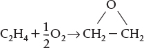
Apparent First-Order Reactions. Because the law of mass action in collision theory shows that two molecules must collide giving a second-order dependence on the rate, you are probably wondering how rate laws such as Equation (3-8) as well as the rate law for first-order reactions come about. An example of first-order reaction not involving radioactive decay is the decomposition of ethanol to form ethylene and hydrogen.
C2H6 → C2H4 + H2
–rC2H6 = kCC2H6
In terms of symbols
A → B + C
–rA = kCA
Rate laws of this form usually involve a number of elementary reactions and at least one active intermediate. An active intermediate is a high-energy molecule that reacts virtually as fast as it is formed. As a result, it is present in very small concentrations. Active intermediates (e.g., A*) can be formed by collision or interaction with other molecules (M) such as inerts or reactants
Here, the activation occurs when translational kinetic energy is transferred into energy stored in internal degrees of freedom, particularly vibrational degrees of freedom.2 An unstable molecule (i.e., active intermediate) is not formed solely as a consequence of the molecule moving at a high velocity (high-translational kinetic energy). The translational kinetic energy must be absorbed into the chemical bonds where high-amplitude oscillations will lead to bond ruptures, molecular rearrangement, and decomposition. In the absence of photochemical effects or similar phenomena, the transfer of translational energy to vibrational energy to produce an active intermediate can occur only as a consequence of molecular collision or interaction. Collision theory is discussed in the Professional Reference Shelf on the CRE Web site for Chapter 3.
As will be shown in Chapter 9, the molecule A becomes activated to A* by collision with another molecule M. The activated molecule can become deactivated by collision with another molecule or the activated molecule can decompose to B and C.
Using this mechanism, we show in Equation (9-10) in Section 9.1.1 that at high concentrations of M, the rate law for this mechanism becomes
and at low concentration of M, the rate law becomes
2 W. J. Moore, Physical Chemistry, Reading, MA: Longman Publishing Group, 1998.
In Chapter 9, we will discuss reaction mechanisms and pathways that lead to nonelementary rate laws, such as the rate of formation of HBr shown in Equation (3-8).
Heterogeneous Reactions. Historically, it has been the practice in many gas–solid catalyzed reactions to write the rate law in terms of partial pressures rather than concentrations. In heterogeneous catalysis it is the weight of catalyst that is important, rather than the reactor volume. Consequently, we use in order to write the rate law in terms of (mol per kg of catalyst per time) in order to design PBRs. An example of a heterogeneous reaction and corresponding rate law is the hydrodemethylation of toluene (T) to form benzene (B) and methane (M) carried out over a solid catalyst
The rate of disappearance of toluene per mass of catalyst, , that is, (mol/mass/time) follows Langmuir-Hinshelwood kinetics (discussed in Section 10.4.2), and the rate law was found experimentally to be
where the prime in denotes typical units are in per kilogram of catalyst (mol/kg-cat/s), PT, PH2, and PB are partial pressures of toluene, hydrogen, and benzene in (kPa, bar or atm), and KB and KT are the adsorption constants for benzene and toluene respectively, with units of kPa–1 (bar–1 or atm–1). The specific reaction rate k has units of
You will find that almost all heterogeneous catalytic reactions will have a term such as (1 + KAPA + ... ) or (1 + KAPA + ... )2 in the denominator of the rate law (cf. Chapter 10).
To express the rate of reaction in terms of concentration rather than partial pressure, we simply substitute for Pi using the ideal gas law
The rate of reaction per unit weight (i.e., mass) catalyst, (e.g., ), and the rate of reaction per unit volume, –rA, are related through the bulk density ρb (mass of solid/volume) of the catalyst particles in the fluid media:
Relating rate per unit volume and rate by per unit mass of catalyst
In “fluidized” catalytic beds, the bulk density, ρb, is normally a function of the volumetric flow rate through the bed.
Consequently, using the above equations for Pi and , we can write the rate law for the hydromethylation of toluene in terms of concentration and in (mole/dm3) and the rate, –rT in terms of reactor volume, that is,
or as we will see in Equation (S4-14) in Chapter 4, we can leave it in terms of partial pressures.
In summary, reaction orders cannot be deduced from reaction stoichiometry. Even though a number of reactions follow elementary rate laws, at least as many reactions do not. One must determine the reaction order from the literature or from experiments.
3.2.3 Reversible Reactions
All rate laws for reversible reactions must reduce to the thermodynamic relationship relating the reacting species concentrations at equilibrium. At equilibrium, the net rate of reaction is identically zero for all species (i.e., –rA ≡ 0). That is, for the general reaction
the concentrations at equilibrium are related by the thermodynamic relationship for the equilibrium constant KC (see Appendix C).
Thermodynamic equilibrium relationship
The units of the thermodynamic concentration equilibrium constant, KC, are (mol/dm3)d+c–b–a.
To illustrate how to write rate laws for reversible reactions, we will use the combination of two benzene molecules to form one molecule of hydrogen and one of diphenyl. In this discussion, we shall consider this gas-phase reaction to be elementary as written and reversible
or, symbolically,
The forward and reverse specific reaction-rate constants, kB and k–B, respectively, will be defined with respect to benzene.
Benzene (B) is being depleted by the forward reaction
in which the rate of disappearance of benzene is
If we multiply both sides of this equation by −1, we obtain the expression for the rate of formation of benzene for the forward reaction
For the reverse reaction between diphenyl (D) and hydrogen (H2),
the rate of formation of benzene is given as
The specific reaction rate constant, ki, must be defined with respect to a particular species.
Again, both the rate constants kB and k–B are defined with respect to benzene!!!
The net rate of formation of benzene is the sum of the rates of formation from the forward reaction [i.e., Equation (3-11)] and the reverse reaction (i.e., Equation (3-12))
Net rate
Multiplying both sides of Equation (3-13) by −1, and then factoring out kB, we obtain the rate law for the rate of disappearance of benzene, –rB
Elementary reversible A ⇄ B
Replacing the ratio of the reverse to forward rate law constants by the reciprocal of the concentration equilibrium constant, KC, we obtain
where
The equilibrium constant decreases with increasing temperature for exothermic reactions and increases with increasing temperature for endothermic reactions.
Let’s write the rate of formation of diphenyl, rD, in terms of the concentrations of hydrogen, H2, diphenyl, D, and benzene, B. The rate of formation of diphenyl, rD, must have the same functional dependence on the reacting species concentrations as does the rate of disappearance of benzene, –rB. The rate of formation of diphenyl is
Using the relationship given by Equation (3-1) for the general reaction
Relative rates
we can obtain the relationship between the various specific reaction rates, kB, kD
Comparing Equations (3-15) and (3-16), we see the relationship between the specific reaction rate with respect to diphenyl, kD, and the specific reaction rate with respect to benzene, kB, is
Consequently, as previously stated, we must define the rate constant, k, with respect to a particular species.
Finally, we need to check to see whether the rate law given by Equation (3-14) is thermodynamically consistent at equilibrium. Applying Equation (3-10) (and Equation (C-2) in Appendix C) to the diphenyl reaction and substituting the appropriate species concentration and exponents, thermodynamics tells us that
Now let’s look at the rate law. At equilibrium, –rB ≡ 0, and the rate law given by Equation (3-14) becomes
At equilibrium, the rate law must reduce to an equation consistent wth thermodynamic equilibrium.
Rearranging, we obtain, as expected, the equilibrium expression
that is identical to Equation (3-17) obtained from thermodynamics.
From Appendix C, Equation (C-9), we know that when there is no change in the total number of moles and the heat capacity term, ΔCP = 0, the temperature dependence of the concentration equilibrium constant is
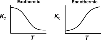
Therefore, if we know the equilibrium constant at one temperature, T1 (i.e., KC (T1)), and the heat of reaction, , we can calculate the equilibrium constant at any other temperature T. For endothermic reactions, the equilibrium constant, KC, increases with increasing temperature; for exothermic reactions, KC decreases with increasing temperature. A further discussion of the equilibrium constant and its thermodynamic relationship is given in Appendix C. For large values of the equilibrium constant, KC, the reaction behaves as if it were irreversible.
3.3 The Reaction-Rate Constant
Concept 1, the law of mass action was discussed in Section 3.2 along with the dependence of the reaction rate on concentration. In this section, we investigate the reaction-rate constant, k, and its temperature dependence using Concept 2, potential energy surfaces and energy barriers, and Concept 3, the energy needed to cross over these barriers.
3.3.1 The Rate Constant k and Its Temperature Dependence
The reaction-rate constant k is not truly a constant; it is merely independent of the concentrations of the species involved in the reaction. The quantity k is referred to as either the specific reaction rate or the rate constant. It is almost always strongly dependent on temperature. It also depends on whether or not a catalyst is present, and in gas-phase reactions, it may be a function of total pressure. In liquid systems, it can also be a function of other parameters, such as ionic strength and choice of solvent. These other variables normally exhibit much less of an effect on the specific reaction rate than does temperature, with the exception of supercritical solvents, such as supercritical water. Consequently, for the purposes of the material presented here, it will be assumed that kA depends only on temperature. This assumption is valid in most laboratory and industrial reactions, and seems to work quite well.
It was the great Nobel Prize-winning Swedish chemist Svante Arrhenius (1859–1927) who first suggested that the temperature dependence of the specific reaction rate, kA, could be correlated by an equation of the type
where A = pre-exponential factor or frequency factor
E = activation energy, J/mol or cal/mol
R = gas constant = 8.314 J/mol · K = 1.987 cal/mol · K
T = absolute temperature, K
(http://www.umich.edu/~elements/6e/03chap/summary.html)
Arrhenius equation
Equation (3-18), known as the Arrhenius equation, has been verified empirically to give the correct temperature behavior of most reaction-rate constants within experimental accuracy over fairly large temperature ranges. The Arrhenius equation is “derived” in section R3.1, Collision Theory, on the CRE Web site (http://www.umich.edu/~elements/6e/03chap/prof-collision.html). One can view the activation energy in terms of collision theory (Professional Reference Shelf R3.1).
By increasing the temperature, we increase the kinetic energy of the reactant molecules. This kinetic energy can in turn be transferred through molecular collisions to internal energy to increase the stretching and bending of the bonds, causing the molecules to reach an activated state, vulnerable to bond breaking and reaction.
3.3.2 Interpretation of the Activation Energy
Why is there an activation energy? If the reactants are free radicals that essentially react immediately on collision, there usually isn’t an activation energy. However, for most atoms and molecules undergoing reaction, there is an activation energy. A couple of the reasons are that in order to react
The molecules need energy to distort or stretch their bonds so that they break and now can form new bonds.
The molecules need energy to overcome the steric and electron repulsive forces as they come close together.
The activation energy can be thought of as a barrier to energy transfer (from kinetic energy to potential energy) between reacting molecules that must be overcome. The activation energy is the minimum increase in potential energy of the reactants that must be provided to transform the reactants into products. This increase can be provided by the kinetic energy of the colliding molecules.
In addition to the concentrations of the reacting species, there are two other factors that affect the rate of reaction:
The height of the potential energy barrier, that is, activation energy
The fraction of molecular collisions that have sufficient energy to cross over the barrier (i.e., react when the molecules collide)
If we have a small barrier height, the molecules colliding will need only low kinetic energies to cross over the barrier. For reactions of molecules with small barrier heights occurring at room temperatures, a greater fraction of molecules will have this energy at low temperatures. However, for larger barrier heights, we require higher temperatures where a higher fraction of colliding molecules will have the necessary energy to cross over the barrier and react. We will discuss each of these concepts separately in Concept 2 and Concept 3.
Concept 2. Potential Energy Surfaces and Energy Barriers. One way to view the barrier to a reaction is through the use of potential energy surfaces and the reaction coordinates. These coordinates denote the minimum potential energy of the system as a function of the progress along the reaction path as we go from reactants to an intermediate to products. For the exothermic reaction
A + BC ⇄ A – B – C → AB + C
the potential energy surface and the reaction coordinate are shown in Figures 3-1 and 3-2. Here EA, EAB, EBC, and EC are the potential surface energies of the reactants (A and BC) and products (AB and C), while EABC is the energy of the complex A–B–C at the top of the barrier shown in Figure 3-2(a).
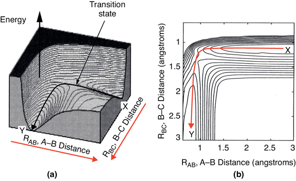
Figure 3-1 A potential energy surface for the H + CH3OH → H2 + CH2OH from the calculations of Blowers and Masel. The lines in the figure are contours of constant energy. The lines are spaced 5 kcal/mol. Richard I. Masel, Chemical Kinetics and Catalysis, p. 370, Fig. 7.6 (Wiley, 2001).
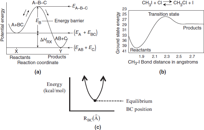
Figure 3-2 Progress along reaction path. (a) Symbolic reaction; (b) Calculated from computational software on the CRE Web site, Chapter 3 Web Module on Molecular Modeling. (c) Side view at point X in Figure 3-1(b), showing the valley.
Figure 3-1(a) shows a 3D plot of the potential energy surface, which is analogous to a mountain pass where we start out in a valley and then climb up to pass over the top of the pass, that is, the col or saddle point, and proceed down into the next valley. Figure 3-1(b) shows a contour plot of the pass and valleys and the reaction coordinate as we pass over the col from valley to valley.
Energy changes as we move within the potential energy surfaces.
At point X in Figure 3-1(b), species A and BC are far apart and are not interacting, and RBC is just the equilibrium bond length between B and C. Consequently, the potential energy is just the BC bond energy. Here, species A and BC are in their minimum potential energy in the valley and the steep rise up from the valley to the col from point X would correspond to increases in the potential energy as A comes close to BC.†
Figure 3-2(c) illustrates when the BC bond is stretched from its equilibrium position at point X, the potential energy increases up one side of the valley hill (RBC increases). The potential energy is now greater because of the attractive forces trying to bring the B–C distance back to its equilibrium position. If the BC bond is compressed at point X from its equilibrium position, the repulsive forces cause the potential energy to increase on the other side of the valley hill, that is, RBC decreases at point X. At the end of the reaction, point Y, the products AB and C are far apart on the valley floor and the potential energy is just the equilibrium AB bond energy. The sides of the valley at point Y represent the cases where AB is either compressed or stretched causing the corresponding increases in potential energy at point Y and can be described in an analogous manner to BC at point X.
We want the minimum energy path across the barrier for converting the kinetic energy of the molecules into potential energy. This path is shown by the curve X→ Y in Figure 3-1 and also by Figure 3-2(a). As we move along the A–B distance axis in Figure 3-2(a), A comes closer to BC, such that A begins to bond with BC and push B and C apart. Consequently, the potential energy of the reaction pair (A and BC) continues to increase until we arrive at the top of the energy barrier, which is the transition state. In the transition state, the molecular distances between A and B and between B and C are close. As a result, the potential energy of the three atoms (molecules) is high. As we proceed further along the arc length of the reaction coordinate depicted in Figure 3-1(a), the AB bond strengthens and the BC bond weakens and C moves away from AB and the energy of the reacting pair decreases until we arrive at the valley floor where AB is far apart from C. The reaction coordinate in Figure 3-2(a) quantifies how far the reaction has progressed. The commercial software available to carry out calculations for the transition state for the real reaction
CH3I + Cl → CH3Cl + I
shown in Figure 3-2(b) is discussed in the Web Module Molecular Modeling in Chemical Reaction Engineering on the CRE Web site (http://www.umich.edu/~elements/6e/web_mod/quantum/index.htm). In addition to Spartan software, which was used to calculate Figure 3-2(b), the software packages, Gaussian 16, IQMol, Q-Chem, and GAMES could be used.
We next discuss the pathway over the barrier shown along the line Y–X. We see that for the reaction to occur, the reactants must overcome the minimum energy barrier, EB, shown in Figure 3-2(a). The energy barrier, EB, is related to the activation energy, E. The energy barrier height, EB, can be calculated from differences in the energies of formation of the transition-state molecule and the energy of formation of the reactants; that is,

The energy of formation of the reactants can be found in the literature or calculated from quantum mechanics, while the energy of formation of the transition state can also be calculated from quantum mechanics using a number of software packages, such as Gaussian (http://www.gaussian.com/) and Dacapo (https://wiki.fysik.dtu.dk/dacapo). The activation energy, E, is often approximated by the barrier height, EB, which is a good approximation in the absence of quantum mechanical tunneling.
† LearnChemE CU video Reaction Coordinate (https://www.youtube.com/watch?v=
Now that we have the general idea for a reaction coordinate, let’s consider another real reaction system
H• + C2H6 → H2 + C2H5•
The energy–reaction coordinate diagram for the reaction between a hydrogen atom and an ethane molecule is shown in Figure 3-3 where the bond distortions, breaking, and forming are identified. This figure shows schematically how the hydrogen molecule, H, moves into CH3–CH3 molecule, distorting the C–H bond and pushing the C–H bond off the methyl hydrogen to arrive at the transition state. As one continues along the reaction coordinate, the methyl hydrogen moves out of the C–H bond into the H–H bond to form the products CH3CH2 and H2.

Figure 3-3 A diagram of the orbital distortions during the reaction
H • + CH3CH3 → H2 + CH2CH3 •
The diagram shows only the interaction with the energy state of ethane (the C–H bond). Other molecular orbitals of the ethane molecule also distort. Courtesy of Richard I. Masel, Chemical Kinetics and Catalysis, p. 594 (Wiley, 2001).
Concept 3. Fraction of Molecular Collisions That Have Sufficient Energy to React. Now that we have established the concept of a barrier height, we need to know what fraction of molecular collisions have sufficient energy to cross over the barrier and react. To discuss this issue, we consider reactions in the gas phase where the reacting molecules will not have only a single velocity, U, but a distribution of velocities, f(U,T). Some will have high velocities and some will have low velocities as they move around and collide. These velocities are not defined with respect to a fixed coordinate system; these velocities are defined with respect to the other reactant molecules. The Maxwell Boltzmann distribution of relative velocities is given by the probability function, f(U, T)
kB = Boltzmann’s constant = 3.29 10–24 cal/molecule/K
m = Reduced mass, g
U = Relative velocity, m/s
T = Absolute Temperature, K
e = Energy kcal/molecule
E = Kinetic energy kcal/mol
We usually interpret f(U, T) with dU, that is,
f(U, T) dU = fraction of reactant molecules with velocities between U and (U + dU).
Rather than using velocities to discuss the fraction of molecules with sufficient energy to cross the barrier, we convert these velocities to energies using the equation for kinetic energy in making this conversion
Using this relationship we substitute, the Maxwell Boltzmann probability distribution of collisions with energy e (cal/molecule) at temperature T is
In terms of energy per mole, E, instead of energy per molecule, e, we have
where E is in (cal/mol), R is in (cal/mol/K), and f(E, T) is in mol/cal.
This function is plotted for two different temperatures in Figure 3-4. The distribution function f(E,T) is most easily interpreted by recognizing that [f(E,T) dE] is the fraction of collision with energies between E and E + dE.
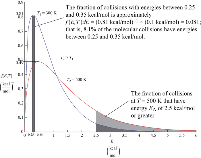
Figure 3-4 Energy distribution of reacting molecules.
For example, the fraction of collisions with energies between 0.25 and 0.35 kcal/mol would be
This fraction is shown by the shaded area in Figure 3-4 and is approximated by the average value of f(E,T) at E = 0.3 kcal/mol which is 0.81 mol/kcal.
Thus 8.1% of the molecular collisions have energies between 0.25 and 0.35 kcal/mol. Go to the Chapter 3 Living Example Problem (LEP) “Variation of Energy Distribution with Temperature” on the Web site and use Wolfram to see how the distribution changes as the temperature changes. Wolfram can be downloaded on your laptop for free (go to http://www.wolfram.com/cdf-player/).
We can also determine the fraction of collisions that have energies greater than a certain value, EA
This fraction is shown in Figure 3-4 by the shaded area for EA = 2.5 kcal/mole for T = 300 K (heavier shade) and for T = 500 K (lighter shade). One can easily see that for T = 500 K a greater fraction of the collisions that cross the barrier with EA = 2.5 kcal/mol and react, which is consistent with our observation that the rates of reaction increase with increasing temperature.
For EA > 3RT, we can obtain an analytical approximation for the fraction of molecules of collision with energies greater than EA by combining Equations (3-21) and (3-22) and integrating to get
Figure 3-5 shows the fraction of collisions that have energies greater than EA as a function of EA for two different temperatures, 300 K and 600 K. One observes for an activation energy EA of 20 kcal/mol and a temperature of 300 K the fraction of collisions with energies greater than 20 kcal/mol is 1.76 × 10⁻¹⁴ while at 600 K, the fraction increases to 2.39 × 10⁻⁷, which is a 7 orders of magnitude difference.
In summary, to explain and give insight to the dependence of rate of reaction on concentration and temperature we introduced three concepts
| Concept 1 | The rate increases with increasing reactant concentration, |
| Concept 2 | The rate is related to the potential energy barrier height and to the conversion of translational energy into potential energy, and |
| Concept 3 | The rate increases with the increasing fraction of collisions that have sufficient energy to cross over the barrier and form products. |
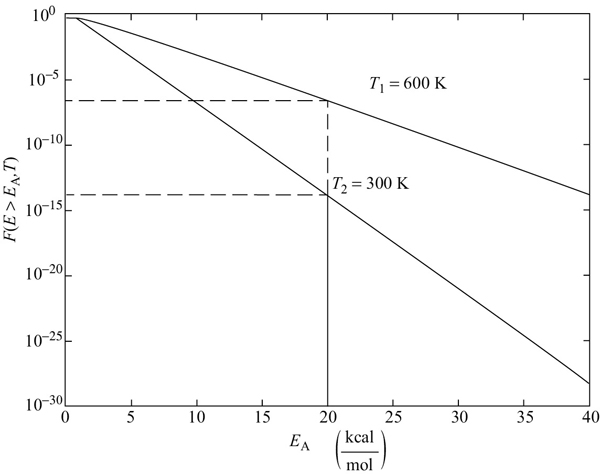
Figure 3-5 Fraction of collision with energies greater than EA.
To carry this discussion to the next level is beyond the scope of this text as it involves averaging over a collection of pairs of molecules to find an average rate with which they pass over the transition state to become products.
Recapping the last section, the energy of the individual molecules falls within a distribution of energies; that is, some molecules have more energy than others. One such distribution is the Boltzmann distribution, shown in Figure 3-4, where f(E, T) is the energy distribution function for the kinetic energies of the reacting molecules. It is interpreted most easily by recognizing the product [f(E, T) dE] as the fraction of molecular collisions that have an energy between E and (E + dE). For example, in Figure 3-4, the fraction of collisions that have energies between 0.25 and 0.35 kcal/mol is 0.081, as shown by the shaded area on the left. The activation energy has been equated with a minimum energy that must be possessed by reacting molecules before the reaction will occur. The fraction of the molecular collisions that have an energy EA or greater is shown by the shaded areas at the right in Figure 3-4. Figure 3-5 shows the fraction of collisions with energies greater than EA as a function of EA at two different temperatures.†
3.3.3 The Arrhenius Plot
Postulation of the Arrhenius‡ equation, Equation (3-18), remains the greatest single advancement in chemical kinetics, and retains its usefulness today, more than a century later. The activation energy, E, is determined experimentally by measuring the reaction rate at several different temperatures. After taking the natural logarithm of Equation (3-18), we obtain
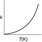
We see that the activation energy can be found from a plot of ln kA as a function of (1/T), which is called an Arrhenius plot. As can be seen in Figure 3-6 the larger the activation energy, the larger the slope and the more temperature-sensitive the reaction. That is, for large E, an increase in just a few degrees in temperature can greatly increase k and thus increase the rate of reaction. The units of kA will depend on the reaction order, and the fact that k in Figure 3-6 has units of s–1 indicates the reaction here is first order.
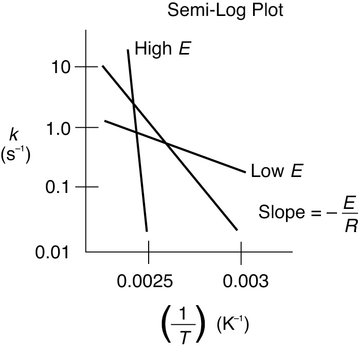
Figure 3-6 Calculation of the activation energy from an Arrhenius plot.
Calculation of the activation energy
† University of Colorado LearnChemE three videos: One on reaction coordinates (https://www.youtube.com/watch?v=Yh9XdLJcTi4) and Mr. Anderson’s activation video (https://www.youtube.com/watch?v=YacsIU97OFc).
‡ Arrhenius bio: http://www.umich.edu/~elements/6e/03chap/summary-bioarr.html.
Example 3–1 Determination of the Activation Energy
Calculate the activation energy for the decomposition of benzene diazonium chlo-ride to give chlorobenzene and nitrogen
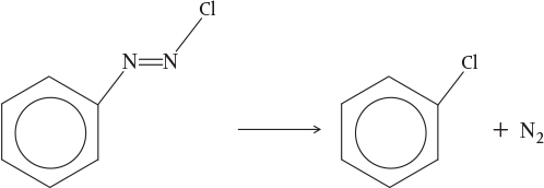
using the information in Table E3-1.1 for this first-order reaction.
TABLE E3-1.1 DATA
k (s–1) |
0.00043 |
0.00103 |
0.00180 |
0.00355 |
0.00717 |
T (K) |
313.0 |
319.0 |
323.0 |
328.0 |
333.0 |
Benzene Diazonium Chloride
Solution
We start by recalling Equation (3-24)

We can use the data in Table E3-1.1 to determine the activation energy, E, and frequency factor, A, in two different ways. One way is to make a semi-log plot of k versus (1/T) and determine E from the slope (–E/R) of an Arrhenius plot. Another way is to use Excel or Polymath to regress the data. The data in Table E3-1.1 was entered in Excel and is shown in Figure E3-1.1, which was then used to obtain Figure E3-1.2.
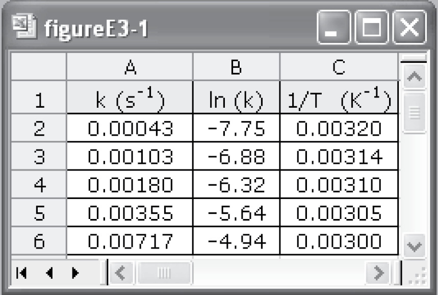
Figure E3-1.1 Excel spreadsheet.
Step-by-step tutorials on how to construct spreadsheets in Polymath and in Excel are on the Web site at http://umich.edu/~elements/6e/software/polymath-tutorial-linearpolyregression.html and http://umich.edu/~elements/6e/live/chapter03/Excel_tutorial.pdf.
Tutorials
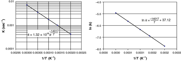
Figure E3-1.2 (a) Excel semi-log plot; (b) Excel normal plot after taking ln(k). (http://www.umich.edu/~elements/6e/software/polymath-tutorial-linearpolyregression.html)
The equation for the best fit of the data
is also shown in Figure E3-1.2(b). From the slope of the line given in Figure E3-1.2(b) and Equation (3-20), we obtain
From Figure E3-1.2(b) and Equation (E3-1.1), we see
ln A = 37.12
Taking the antilog, we find the frequency factor to be
A 1.32 × 10¹⁶ s–1
Analysis: The activation energy, E, and frequency factor, A, can be calculated if we know the specific reaction rate, k, at two temperatures, T1 and T2. We can either use the Arrhenius equation (3-18) twice, once at T1 and once at T2, to solve two equations for the two unknowns, A and E, or we can take the slope of a plot of (ln k) as a function of (1/T); the slope will be equal to (–E/R).
There is a rule of thumb that states that the rate of reaction doubles for every 10°C increase in temperature. However, this rule is true only for specific combinations of activation energies and temperatures. For example, if the activation energy is 53.6 kJ/mol, the rate will double only if the temperature is raised from 300 to 310 K. If the activation energy is 147 kJ/mol, the rule will be valid only if the temperature is raised from 500 to 510 K (see Problem P3-10B for the derivation of this relationship).
The rate does not always double for a temperature increase of 10°C.

The larger the activation energy, the more temperature-sensitive is the rate of reaction. While there are no typical values of the frequency factor and activation energy for a first-order gas-phase reaction, if one were forced to make a guess, values of A and E might be 1013 s–1 and 100 kJ/mol. However, for families of reactions (e.g., halogenation), a number of correlations can be used to estimate the activation energy. One such correlation is the Polanyi-Semenov equation, which relates activation energy to the heat of reaction (see Collision Theory in Professional Reference Shelf R3.1 [http://www.umich.edu/~elements/6e/03chap/prof-collision.html#VI]). Another correlation relates the activation energy to differences in bond strengths between products and reactants.3 While the activation energy cannot be currently predicted a priori, significant research efforts are under way to calculate activation energies from first principles.4
One final comment on the Arrhenius equation, Equation (3-18). It can be put in a most useful form by finding the specific reaction rate at a temperature T0; that is,
k (T0) = Ae–E/RT0
and at a temperature T
k (T) = Ae–E/RT
and taking the ratio to obtain
A most useful form of k(T)
This equation says that if we know the specific reaction rate k(T0) at a temperature, T0, and we know the activation energy, E, we can find the specific reaction rate k(T) at any other temperature, T, for that reaction.
3 M. Boudart, Kinetics of Chemical Processes, Upper Saddle River, NJ: Prentice Hall, p. 168. J. W. Moore and R. G. Pearson, Kinetics and Mechanisms, 3rd ed. New York: Wiley, p. 199. S. W. Benson, Thermochemical Kinetics, 2nd ed. New York: Wiley.
4 R. Masel, Chemical Kinetics and Catalysis, New York: Wiley, 2001, p. 594.
3.4 Molecular Simulations
3.4.1 Historical Perspective
For the last 10 years or so, molecular simulations have been used more and more to help understand chemical reactions along with their pathways and mechanisms. Consequently, to introduce you to this area, we will use MATLAB to simulate a simple reaction and view a couple of molecular simulation trajectories. Some of the earliest simulations were carried out by Professor Martin Karplus more than 50 years ago and are described in his groundbreaking journal article J. Chem. Phys., 43, 3259 (1965) for the reaction
A + BC → AB + C
The forces and potential energies he used to describe the interaction as the two molecules approach each other are described in the Professional Reference Shelf R3.3 Molecular Dynamics (PRS R3.3) (http://www.umich.edu/~elements/6e/03chap/prof-moldyn.html).
In Karplus’s procedure, the trajectories and molecular collisions of species A and BC are calculated and analyzed to determine whether or not they have sufficient translational, vibrational, and kinetic energy, along with molecular orientation to either react or not react. A nonreactive trajectory and a reactive trajectory are shown in Figures 3-7(a) and 3-7(b), respectively. One notes the vibrations of the AB and BC molecules from the plot of RAB and RBC with time. In the Monte Carlo simulation, the randomly chosen input parameters are (1) the initial distance between A and BC, (2) the orientation of BC relative to A, and (3) the angular momentum of BC. Next, the reaction trajectories are calculated to learn whether the trajectory is reactive or nonreactive and the result is recorded. This process is repeated a number of times for different random input parameters and the number of reactive and nonreactive trajectories for these input parameters are again counted and recorded. The statistics of the number of reactive versus number of nonreactive trajectories are then used to develop a probability of reaction. The specific reaction-rate constant and the activation energy are determined from the probability of reaction (cf. PRS R3.3).
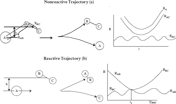
Figure 3-7 Molecular Trajectories (a) Nonreactive (b) Reactive.
Professor Karplus received the 2013 Nobel Prize for his pioneering work in molecular simulations.
3.4.2 Stochastic Modeling of Reactions†
However, rather than tracking singular trajectories as Karplus did, we consider an ensemble of molecules and the collisions between both reactants and products and use stochastic modeling to determine the concentration trajectories of the reacting molecules. To illustrate the stochastic modeling of chemical reactions, we will use the reversible reaction
which we will write as separate reactions
Reaction (1)
Reaction (2)
that are assumed to be elementary and have deterministic rate laws given by –rA = kfCACB and –rC = krCCCD.
To model these reactions stochastically, we define the probability that the “reaction i” will occur per unit time, that is, ri. This probability is related to the number of ways the reaction can occur per unit time, which is analogous to the deterministic rate law. The probability function of Reaction (1) occurring per unit time, rf, is
and the probability function of Reaction (2) occurring per unit time is
where the terms xi are the number of molecules of species i. Here rf and rr are the probability functions of the forward and the reverse reactions occurring per unit time and the rate constants kf and kr are probabilities that the collisions between molecules A and B give rise to Reaction (1) or between molecules C and D giving rise to Reaction (2) respectively. The rate constants kf and kr have units of . The total reaction probability function, rt, is
† An overview of stochastic modeling can be found in a PowerPoint presentation on the Web site (http://www.doc.ic.ac.uk/~jb/conferences/pasta2006/slides/stochastic-simulation-introduction.pdf).
In carrying out the stochastic simulations, we randomly choose which reaction, that is, either (1) or (2), will occur in time step ti based on the reactive probabilities of each of the two reactions. The probability of Reaction (1) occurring is related to the ratio
and the probability of Reaction (2) occurring is related to the ratio
Next, we generate a random number, p1, in the interval (0, 1). If the random number p1 is less than f1, that is, (0 ≤ p1 ≤ f1) then Reaction (1) occurs and the number of A and B molecules decrease by one each and the number of C and D molecules increase by one each and these numbers are then recorded at time ti. If p1 was not in that interval (0 ≤ p1 < f1), then Reaction (2) occurs and the number of A and B molecules each increase by one and the number of C and D molecules each decrease by one. Consequently, the probability values of f1 and f2 will change for the next time step and for the next random number generation. Let’s consider the first six-time steps in which the probability results show that Reaction (1) takes place in the first three-time steps, while Reaction (2) occurs in the fourth- and fifth-time steps, and then Reaction (1) occurs again in the sixth-time step. The number of C or D molecules after the first six steps are 1 → 2 → 3 → 2 → 1 → 2 as shown in Figure 3-8 (a) as a function of the step numbers, that is, i.
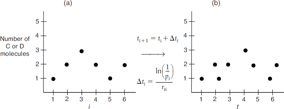
Figure 3-8 (a) Number of molecules as a function of a simulation run number i. (b)Number of molecules as a function of time, where rti is the total rate at time ti.
We now will convert the step number to a time t. The time between a molecular collision of A and B is also random. To determine this time, we use the random number generated for simulation run number i, pi (0 < pi < 1). The corresponding time increment is
Where Equation (3-28) is evaluated at step i, Δti has the units of seconds. We update the time t by the equation
Figure 3-8(b) shows the number of C or D molecules as a function of time after the Figure 3-8(a) axis is converted to time using Equations (3-31) and (3-32).
If we continued the time steps in this fashion, the overall number of C and D molecules would continue to increase in a stochastic manner as shown in Figure 3-9(b). Analogously, the number of A and B molecules would continue to decrease, also shown in this figure.

Figure 3-9(a) Graphical user interface in LEP.
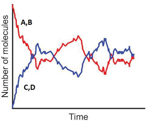
Figure 3-9(b) Molecular trajectories.
Stochastic modeling allows us to see on a molecular level how the reaction progresses. The takeaway lesson is that while the deterministic model shows the smooth reaction path of species C and D being formed, on the molecular scale we see C and D being formed, then reacting back to A and B and then being formed again.
Figure 3-9(b) shows how the number of molecules of species A and C fluctuate as the reaction progresses.
Now carry out the simulation by going to the Web, load the Chapter 3 LEP on molecular simulations and use the Graphical User Interface shown in Figure 3-9(a). Vary the number of molecules initially along with rate constants kf and kr (cf. LEP P3-1A (b)) and observe the trajectories similar to the one shown in Figure 3-9(b). A tutorial on how to run the simulation is given on the Web site along with the simulation of a series reaction (A + B ⇄ C + D ⇄ E + F).
3.5 Present Status of Our Approach to Reactor Sizing and Design
In Chapter 2, we combined the different reactor mole balances with the definition of conversion to arrive at the design equation for each of four types of reactors, as shown in Table 3-2. Next we showed that if the rate of disappearance is known as a function of the conversion X
–rA = g (X)
then it is possible to size CSTRs, PFRs, and PBRs operated at the same conditions under which –rA = g(X) was obtained.
In general, information in the form –rA = g(X) is not available. However, we have seen in Section 3.2 that the rate of disappearance of A, –rA, is normally expressed in terms of the concentration of the reacting species. This functionality
TABLE 3-2 DESIGN EQUATIONS
Differential Form |
Algebraic Form |
Integral Form |
|
Batch |
|||
Backmix (CSTR) |
|||
Fluidized CSTR |
|||
Tubular (PFR) |
|||
Packed bed (PBR) |
The design equations
is called a rate law. In Chapter 4, we show how the concentration of the reacting species may be written in terms of the conversion X
and then we can design isothermal reactors
With these additional relationships, one observes that if the rate law is given and the concentrations can be expressed as a function of conversion, then in fact we have –rA as a function of X and this is all that is needed to evaluate the isothermal design equations. One can use either the numerical techniques described in Chapter 2 or, as we shall see in Chapter 5, a table of integrals, and/or software programs (e.g., Polymath).
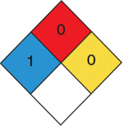
3.6 And Now... A Word from Our Sponsor–Safety 3 (AWFOS–S3 The GHS Diamond)
The National Fire Protection Association (NFPA) diamond discussed in AWFOS–S2 is most commonly used in the United States, but is rarely used in Europe and other countries where the Globally Harmonized System (GHS) diamond is more common. While it is not legally required to use the GHS or the NFPA labeling systems, it is required that chemical containers do have some form of hazard identification on them that comply with the HazCom 2012 standards developed by the Occupation Safety and Health Administration (OSHA) (https://www.osha.gov/law-regs.html). Because countries in Europe and other countries use the GHS labeling system, this AWFOS–S outlines the GHS system that makes the import and export of chemicals easier and safer. The GHS system uses three categories of hazards rather than four like NFPA uses. The three different categories are flammables, health hazards, and environmental hazards and uses nine different pictograms, as shown in Figure 3-10. These pictograms are placed on containers to identify the hazard of the chemical being stored in the container. The Web site Process Safety Across the Chemical Engineering Curriculum (http://umich.edu/~safeche/nfpa.html) gives an excellent discussion along with many examples for each of the nine diamonds. We should note however that there are variations of the pictograms and the rules of when to use what variation of the labels can be found on pages 38–42 of the PDF document found on the Web site https://www.osha.gov/dsg/hazcom/ghsguideoct05.pdf.
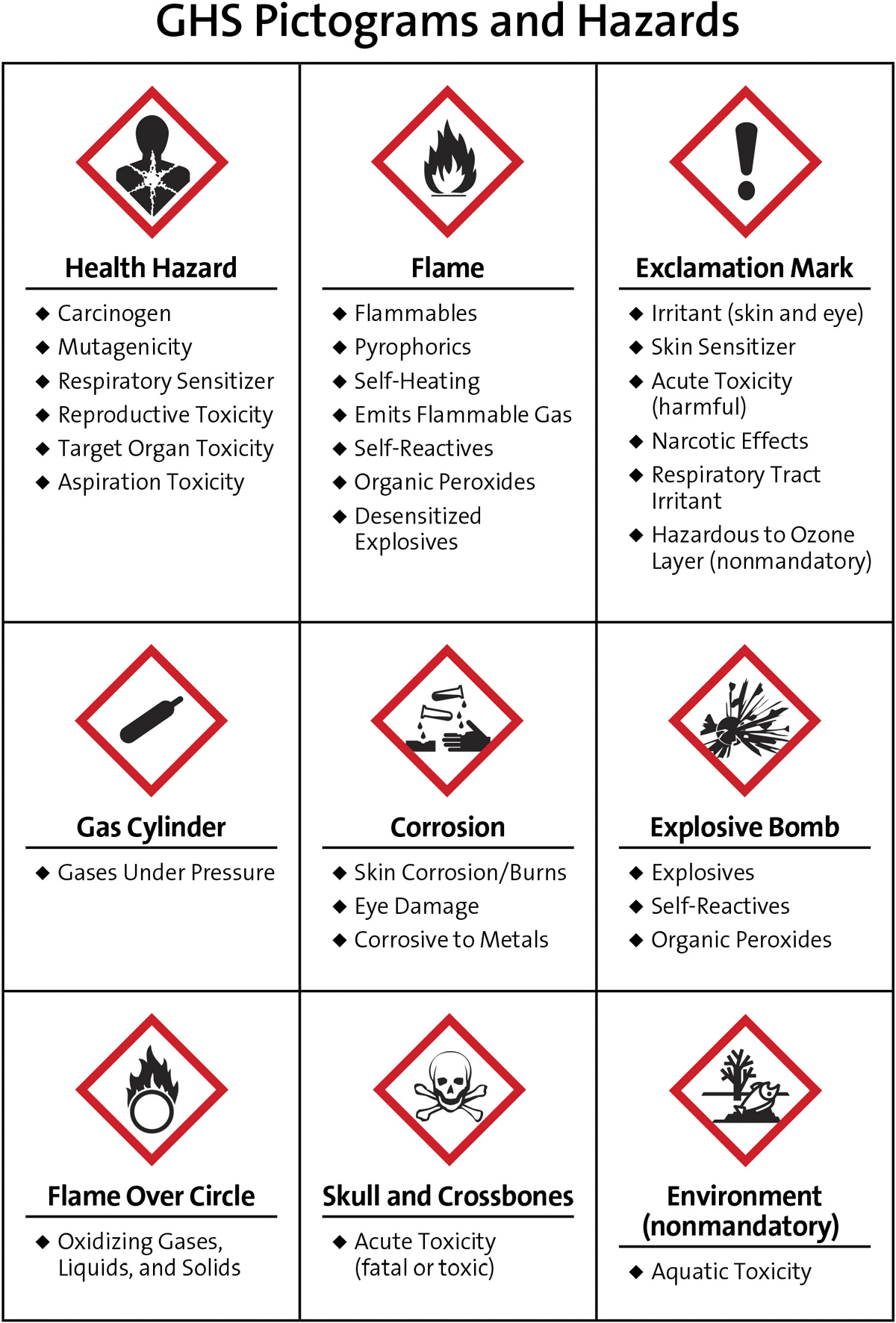
Figure 3-10 Pictograms from the GHS Labeling.†
†Courtesy of American Chemical Society Eighth Edition of Safety in Academic Chemistry Laboratories: Best Practices for First- and Second-Year University Students, ACS, 1155 Sixteenth Street NW, Washington, DC 20036.
Many companies in the United States are changing from the NFPA labeling system to the GHS system (Figure 3-11).
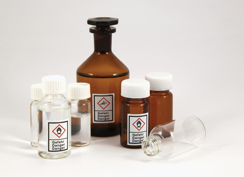
Figure 3-11 The GHS in action. (Photo by fotosommer, Panther Media GmbH/Alamy Stock Photo) (https://www.bradyid.com/applications/ghs-labeling-requirements)†
Closure. Having completed this chapter, you should be able to write the rate law in terms of concentration and the Arrhenius temperature dependence. We have now completed the first two basic building blocks in our algorithm to study isothermal chemical reactions and reactors.

In Chapter 4, we focus on the third building block, stoichiometry, as we use the stoichiometric table to write the concentrations in terms of conversion to finally arrive at a relationship between the rate of reaction and conversion.
The CRE Algorithm
Mole Balance, Ch 1
Rate Law, Ch 3
Stoichiometry, Ch 4
Combine, Ch 5
Evaluate, Ch 5
Energy Balance, Ch 11
Summary
Relative rates of reaction for the generic reaction:
The relative rates of reaction can be written either as
†Courtesy of American Chemical Society Eighth Edition of Safety in Academic Chemistry Laboratories: Best Practices for First- and Second-Year University Students, ACS, 1155 Sixteenth Street NW, Washington, DC 20036.
Reaction order is determined from experimental observation:
The reaction in Equation (S3-3) is α order with respect to species A and β order with respect to species B, whereas the overall order, n, is (α + β). If α = 1 and β = 2, we would say that the reaction is first order with respect to A, second order with respect to B, and overall third order. We say a reaction follows an elementary rate law if the reaction orders agree with the stoichiometric coefficients for the reaction as written.
Examples of reactions that follow an elementary rate law:
Irreversible reactions
First order
Second order
Reversible reactions
Second order
Examples of reactions that follow nonelementary rate laws:
Homogeneous
Heterogeneous reactions
The temperature dependence of a specific reaction rate is given by the Arrhenius equation
where A is the frequency factor and E the activation energy.
If we know the specific reaction rate, k, at a temperature, T0, and the activation energy, we can find k at any temperature, T
Concept 1 The rate increases with increasing reactant concentrations, Concept 2 The rate is related to the potential barrier height and to the conversion of translational energy into potential energy, and Concept 3 The rate increases as the fraction of collisions that have sufficient energy to cross over the barrier and form products increases. Similarly from Appendix C, Equation (C-9), if we know the partial pressure equilibrium constant KP at a temperature, T1, and the heat of reaction, we can find the equilibrium constant at any other temperature
CRE Web Site Materials
(http://www.umich.edu/~elements/6e/04chap/obj.html#/)

Web Module
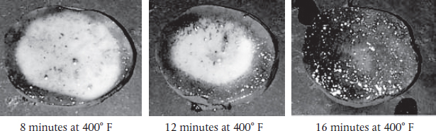
A. Chemical reaction engineering is applied to cooking a potato (http://www.umich.edu/~elements/6e/web_mod/potato/index.htm)
with
k = Ae–E/RT
• Professional Reference Shelf (http://umich.edu/~elements/6e/03chap/prof.html)
R3.1 Collision Theory (http://umich.edu/~elements/6e/03chap/prof-collision.html)
In this section, the fundamentals of collision theory are applied to the reaction
A + B → C + D
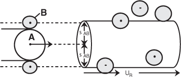
Figure R3.1 Schematic of collision cross section.
to arrive at the following rate law
The activation energy, EA, can be estimated from the Polanyi equation
R3.2 Transition-State Theory (http://umich.edu/~elements/6e/03chap/prof-transition.html)
In this section, the rate law and rate-law parameters are derived for the reaction
A + BC ⇄ ABC# → AB + C
using transition-state theory. Figure R3.2 shows the energy of the molecules along the reaction coordinate, which measures the progress of the reaction.

Figure R3.2 Reaction coordinate for (a) SN2 reaction, and (b) generalized reaction. (c) 3-D energy surface for generalized reaction.
R3.3 Molecular Dynamics Simulations (http://umich.edu/~elements/6e/03chap/prof-moldyn.html)
The reaction trajectories are calculated to determine the reaction cross section of the reacting molecules. These trajectories, which are identified as either (1) nonreactive or (2) reactive, are shown in Figure 3-7. The reaction probability is found by counting up the number of reactive trajectories after Karplus.† Professor Karplus received the 2013 Nobel Prize for his work on Molecular Dynamic Simulations.
Questions, Simulations, and Problems
The subscript to each of the problem numbers indicates the level of difficulty: A, least difficult; D, most difficult.
A = • B = ▪ C = ♦ D = ♦ ♦

Questions
Q3-1A QBR (Question Before Reading). How do you think the rate of reaction, –rA, will depend on species concentrations and on temperature?
Q3-2A i>clicker. Go to the Web site (http://www.umich.edu/~elements/6e/03chap/iclicker_ch3_q1.html) and view at least five i>clicker questions. Choose one that could be used as is, or a variation thereof, to be included on the next exam. You also could consider the opposite case: explain why the question should not be on the next exam. For either case, explain your reasoning.
† M. Karplus, R. N. Porter, and R. D. Sharma, J. Chem. Phys., 43 (9), 3259 (1965).
Q3-3C (a) List the important concepts that you learned from this chapter. What concepts are you not clear about?
Explain the strategy to evaluate reactor design equations and how this chapter expands on Chapter 2.
The rate law for the reaction . What are kB and kC?
Listen to the audios
 on the CRE Web site. Select a topic and explain it.
Which example on the CRE Web site’s Summary Notes for Chapters 1 through 3 was most helpful?
Q3-4A How would you rate the level importance of the GHS diamonds from 1 to 9 (9 being highest). For example, is having the gas cylinder label more important than exclamation mark, if so, why? What are the GHS symbols for ethylene oxide?
Q3-5A Go to the LearnChemE screencast link for Chapter 3 (http://www.umich.edu/~elements/6e/03chap/learn-cheme-videos.html).
View one of the screencast 5- to 6-minute video tutorials and list two of the most important points.
In Professor Andersen’s video, what are the reaction orders wrt A and to B?
Q3-6A AWFOS–S3 Could you, if possible, fit the various nine GHS diamonds into the four NFPA diamonds?
Q3-7B It was a dark late August night with a full moon. Nevertheless, not fearing for my own safety as to what might be lurking, I took my voice recorder outside where I followed the sound to a nearby bush and made the following recording (http://www.umich.edu/~elements/6e/03chap/summary-selftest1.html).
What was the temperature to which I was exposed to? Hint: Problem P3-7A may be of help or see Big Bang Theory episode for Sheldon Cooper’s cricket analysis (https://www.youtube.com/watch?v=prafMmD_mx8).
The following government Web site (https://www.loc.gov/rr/scitech/mysteries/cricket.html) alludes to a correlation of chips and temperature. Can you derive that correlation using the Arrhenius Equation?
Computer Simulations and Experiments
P3-1B (a) LEP: Variation of Energy Distribution with Temperature.
Wolfram and Python
Vary temperature, T, and activation energy, E, to learn their effects on energy distribution curve. Specifically, vary the parameters between their maximum and minimum values (i.e., high T, low E; low T, low E; high T, high E; etc.) and write a few sentences describing what you find.
What should be the minimum temperature so that at least 50% molecules have energy greater than the activation energy you have chosen (e.g., 6 kcal/mol)?
After reviewing Generating Ideas and Solutions on the Web site (http://www.umich.edu/~elements/6e/toc/SCPS,3rdEdBook(Ch07).pdf). Choose one of the brainstorming techniques (e.g., lateral thinking) to suggest two questions that should be included in this problem.
(b) MATLAB Chemical Kinetics Simulations. Go to the Chapter 3 LEPs and choose LEP-Mol-Sim.Zip and carry out the following parameter variations. Before you run the simulation the first time, you will probably want to go through the tutorial.
For kf = kr = 1.0 Run the simulation when the number of A and B are
A = 20 B = 20 C = D = 0
A = 200 B = 200 C = D = 0
A = 2,000 B = 2,000 C = D = 0
A = 200 B = 2,000 C = D = 0
Is there any effect of the experiments (a)–(d) on the equilibrium concentration? What about the time taken to attain equilibrium?
What conclusions do you draw from your experiments?
For 100 A molecules and 100 B molecules, vary the specific reaction–rate constants kf and kr and describe the differences in trajectories you observe.
What happens when you set either kf or kr to zero?
Why are there fluctuations in the concentration trajectories? Why are they not smooth? What causes the size of the fluctuations to increase or decrease?
What do you observe when you increase the initial number of molecules? Can you explain your observations?
Do the reactions stop once equilibrium is reached?
Write a conclusion on what you found in experiments (i)–(vi).
Problems
P3-2B Exploring the Example Problems.
Example 3-1. Activation Energy. In the Excel spreadsheet, replace the value of k at 312.5 K with k = 0.0009–1s and determine the new values of E and k.
Example 3-1. Make a plot of k versus T and ln k versus (1/T) for E = 240 kJ/mol and for E = 60 kJ/mol. (1) Write a couple of sentences describing what you find. (2) Next, write a paragraph describing the activation energy and how it affects chemical reaction rates, and what its origins are.
Collision Theory—Professional Reference Shelf. Make an outline of the steps that were used to derive
–rA = Ae–E/RT CACB
P3-3B OEQ (Old Exam Question). Molecular collision energies—refer to Figure 3-4 and to the Wolfram and Python LEP 3-1. cdf Variation of Energy Distribution with Temperature.
What fraction of molecular collisions have energies less than or equal to 2.5 kcal at 300 K? At 500 K?
What fraction of molecular collisions have energies between 3 and 4 kcal/mol at T = 300 K? At T = 500 K?
What fraction of molecular collisions have energies greater than the activation energy EA = 25 kcal at T = 300 K? At T = 500 K?
P3-4B
Use Figure 3-1(b) to sketch the trajectory over the saddle point when the BC and AB molecules vibrate with the minimum separation distance being 0.20 Angstroms and the maximum separation being 0.4 Angstroms.
At point Y, RAB = 2.8 Angstroms, sketch the potential energy as a function of the distance RBC noting the minimum at valley floor.
At Point X, RBC = 2.8 Angstroms, sketch the potential energy as a function of RAB noting the minimum on the valley floor.
P3-5B Use Equation (3-20) to make a plot of f(E,T) as a function of E for T = 300, 500, 800, and 1200 K.
What is the fraction of molecules that have sufficient energy to pass over a energy barrier of 25 kcal at 300, 500, 800, and 1200 K?
For a temperature of 300 K, what is the ratio of the faction of energies between 15 and 25 kcal to that for the same energy range (15–25 kcal) at 1200 K?
Make a plot of F(E > EA,T) as a function of (EA/RT) for (EA/RT) > 3. What is the fraction of collisions that have energies greater than 25 kcal/mole at 700 K?
What fraction of molecules have energies greater than 15 kcal/mol at 500 K?
Construct a plot of F(E > EA,T) versus T for EA = 3, 10, 25, and 40 kcal/mole. Describe what you find. Hint: Recall the range of validity for T in Equation (3-23).
P3-6A OEQ (Old Exam Question). The following figures show the energy distribution function at 300 K for the reaction A + B → C.
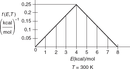
Figure P3-6(a)
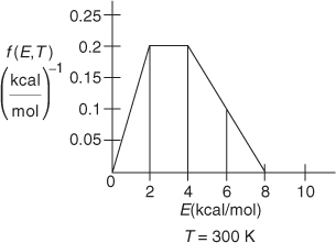
Figure P3-6(b)
For each figure, determine the following:
What fraction of the collisions have energies between 3 and 5 kcal/mol?
What fraction of collisions have energies greater than 5 kcal/mol? (Ans: Figure P3-6 (b) fraction = 0.28)
What is the fraction with energies greater than 0 kcal/mol?
What is the fraction with energies 8 kcal/mol or greater?
If the activation energy for Figure P3-6(b) is 8 kcal/mol, what fraction of molecules have an energy greater than EA?
Guess what (sketch) the shape of the curve f(E,T) versus E shown in Figure P3-6(b) would look like if the temperature were increased to 400 K. (Remember: .)
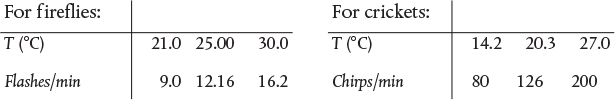
P3-7A The frequency of fireflies flashing and the frequency of crickets chirping as a function of temperature follow. Source: Keith J. Laidler, “Unconventional applications of the Arrhenius law.” J. Chem. Educ., 5, 343 (1972). Copyright (c) 1972, American Chemical Society. Reprinted by permission.

The running speed of ants and the flight speed of honeybees as a function of temperature are given below. Source: B. Heinrich, The Hot-Blooded Insects, Cambridge, MA: Harvard University Press, 1993.
For ants: |
|
For honeybees: |
||||||||
T (°C) |
10 |
20 |
30 |
38 |
|
T (°C) |
25 |
30 |
35 |
40 |
V (cm/s) |
0.5 |
2 |
3.4 |
6.5 |
|
V (cm/s) |
0.7 |
1.8 |
3 |
? |
What do the firefly and cricket have in common? What are their differences?
What is the velocity of the honeybee at 40°C? At –5°C?
Nicolas wants to know if the bees, ants, crickets, and fireflies have anything in common. If so, what is it? You may also do a pair-wise comparison.
Would more data help clarify the relationships among frequency, speed, and temperature? If so, in what temperature should the data be obtained? Pick an insect, and explain how you would carry out the experiment to obtain more data. For an alternative to this problem, see CDP3-AB.
Data on the tenebrionid beetle whose body mass is 3.3 g show that it can push a 35-g ball of dung at 6.5 cm/s at 27°C, 13 cm/s at 37°C, and 18 cm/s at 40°C.
How fast can it push dung at 41.5° C? Source: B. Heinrich. The Hot-Blooded Insects, Cambridge, MA: Harvard University Press, 1993. (Ans: 19.2 cm/s at 41.5°C)

Use http://www.umich.edu/~scps/html/probsolv/strategy/cteq.htm to write three critical thinking questions and three creative questions.
P3-8B OEQ (Old Exam Question). Troubleshooting. Corrosion of high-nickel stainless steel plates was found to occur in a distillation column used at DuPont to separate HCN and water. Sulfuric acid is always added at the top of the column to prevent polymerization of HCN. Water collects at the bottom of the column and HCN collects at the top. The amount of corrosion on each tray is shown in Figure P3-8B as a function of plate location in the column.

Figure P3-8B Corrosion in a distillation column.
The bottommost temperature of the column is approximately 125°C and the topmost is 100°C. The corrosion rate is a function of temperature and the concentration of an HCN–H2SO4 complex.
Suggest an explanation for the observed corrosion-plate profile in the column. What effect would the column operating conditions have on the corrosion-plate profile?
Identify the components of the GHS diagram that you could apply to this problem.
P3-9B Inspector Sgt. Ambercromby of Scotland Yard. It is believed, although never proven, that Bonnie murdered her first husband, Lefty, by poisoning the tepid brandy they drank together on their first anniversary. Lefty was unaware she had coated her glass with an antidote before she filled both glasses with the poisoned brandy. Bonnie married her second husband, Clyde, and some years later when she had tired of him, she called him one day to tell him of her new promotion at work and to suggest that they celebrate with a glass of brandy that evening. She had the fatal end in mind for Clyde. However, Clyde suggested that instead of brandy, they celebrate with ice-cold Russian vodka and down it Cossack style, in one gulp. She agreed and decided to follow her previously successful plan and to put the poison in the vodka and the antidote in her glass. The next day, both were found dead. Sgt. Ambercromby arrives #Seriously? What are the first three questions he asks? What are two possible explanations? Based on what you learned from this chapter, what do you feel Sgt. Ambercromby suggested as the most logical explanation?

Who done it?
Source: Professor Flavio Marin Flores, ITESM, Monterrey, Mexico. Hint: View the YouTube video (www.youtube.com) made by the chemical reaction engineering students at the University of Alabama, titled The Black Widow. You can access it from the CRE Web site (www.umich.edu/~elements/6e) using the YouTube Videos link under By Concepts on the CRE home page.
P3-10B Activation Energy
The rule of thumb that the rate of reaction doubles for a 10°C increase in temperature occurs only at a specific temperature for a given activation energy. Develop a relationship between the temperature and activation energy for which the rule of thumb holds. Neglect any variations in concentrations. For EA = 50 kcal/mol, over what temperature range (T2 = T1 + 10°C) is this rule of thumb valid?

Write a paragraph explaining activation energy, E, and how it affects the chemical reaction rate. Refer to Section 3.3 and especially the Professional Reference Shelf Sections R3.1, R3.2, and R3.3 if necessary.
P3-11C The initial reaction rate for the elementary reaction
2A + B → 4C
was measured as a function of temperature when the concentration of A was 2 M and that of B was 1.5 M.
–rA(mol/dm3 · s): |
0.002 |
0.046 |
0.72 |
8.33 |
T(K): |
300 |
320 |
340 |
360 |
What is the activation energy?
What is the frequency factor?
What is the rate constant as a function of temperature using Equation (S3-5) and T0 = 27°C as the base case?
P3-12B Determine the rate law for the reaction described in each of the cases below involving species A, B, and C. The rate laws should be elementary as written for reactions that are either of the form A → B or A + B → C.
The units of the specific reaction rate are : Rate Law ______
The units of the specific reaction rate are : Rate Law _____
The units of the specific reaction rate are : Rate Law ______
The units of a nonelementary reaction rate are : Rate Law _________
P3-13A (a) Write the rate law for the following reactions assuming each reaction follows an elementary rate law. Give the units of kA for each, keeping in mind some are homogeneous and some reactants are heterogeneous.
C2H6 → C2H4 + H2
(CH3)3COOC (CH3)3 ⇄ C2 H6 + 2CH3COCH3
nC4H10 ⇄ iC4H10
CH3COOC2H5 + C4H9OH ⇄ CH3COOC4H9 + C2H5OH
(CH3CO)2O + H2O ⇄ 2CH3COOH
P3-14A
OEQ (Old Exam Questions). Write the rate law for the reaction
2A + B → C
if the reaction
is second order in B and overall third order, –rA = ______
is zero order in A and first order in B, –rA = ______
is zero order in both A and B, –rA = ______
is first order in A and overall zero order, –rA = ______
Find and write the rate laws for the following reactions:
H2 + Br2 → 2HBr
H2 + I2 → 2HI
Hint: See Chapter 9 Learning Resources: A. Hydrogen Bromide.
P3-15B The rate laws for each of the reactions listed below were obtained at low temperatures. The reactions are highly exothermic and therefore reversible at high temperatures. Suggest a rate law for each of the reactions [(a), (b), and (c)] at high temperatures, which may or may not be elementary.
The reaction
A → B
is irreversible at low temperatures and the rate law is
–rA = kCA
The reaction
A + 2B → 2D
is irreversible at low temperatures and the rate law is
–rA = kCA1/2 CB
The gas–solid catalyzed reaction
is irreversible at low temperatures and the rate law is
In each case, make sure that the rate laws at high temperatures are thermodynamically consistant at equilibrium (cf. Appendix C).
P3-16B Solar Chemical Energy Storage. The major ways to utilize, capture, or store the sun’s energy are solar thermal (see Problem P8-16B), solar voltaic, biomass conversion, solar water splitting (Problem P10-13B), and solar chemical. Solar chemical refers to processes that harness and store solar energy by adsorbing light in a reversible chemical reaction; see http://en.wikipedia.org/wiki/Solar_chemical. For example, the photodimerization of anthracene absorbs and stores solar energy that can be released when the reverse reaction takes place.
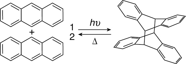
Figure P3-16.1 Anthracene dimerization.
Another reaction of interest is the Norbornadiene–Quadricyclane (NQ) couple, where solar energy is adsorbed and stored in one direction and released in the other.
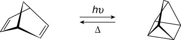
Figure P3-16.2 The Norbornadiene– Quadricyclane (NQ) couple is of potential interest for sunlight energy storage.
Suggest a rate law for the reversible photodimerization of anthracene.
Suggest a rate law for the reversible storage of energy by the NQ couple.
Supplementary Reading
Two references relating to the discussion of activation energy have already been cited in this chapter. Activation energy is usually discussed in terms of either collision theory or transition-state theory. A concise and readable account of these two theories may or may not be found in
THORNTON W. BURGESS, The Adventures of Reddy Fox. New York: Dover Publications, Inc., 1913.
K. J. LAIDLER, Chemical Kinetics. New York: Harper & Row, 1987, Chap. 3.
R. MASEL, Chemical Kinetics and Catalysis. New York: Wiley, 2001, p. 594.
Prof. Dr. Sven Köttlov of Jofostan University has pointed out that in addition to the books listed above, the rate laws and activation energies can be found in NBS circulars, such as those shown below Table 3-1 on pages 81–82. Also check chemistry literature, for example, Journal of Physical Chemistry. For more on molecular modeling, see http://cache.org/teaching-resources-center/molecular-modeling.