
Introduction
Abstract
Embedded system interfacing is the conceptual interface between electrical and computer engineering—we require the skills of both fields to design good, practical interfaces. I/O is particularly important to embedded computing systems. Embedded computers are responsible for a wide range of devices, ranging from simple appliances to complex vehicles and industrial equipment. This range of I/O requirements calls for a comprehensive playbook of interfacing techniques. This chapter surveys embedded system interfacing methods and reviews basic principles of circuit analysis.
Keywords
Embedded system; Interfacing; Mixed-signal; Hardware/software codesign; Analog circuits; Digital logic
1.1 Interfacing Computers to the Physical World
Useful computers need some sort of input and output. Computation that we can’t see doesn’t provide much attraction. Early computers used primitive I/O devices: lights, paper tape, crude displays. The development of new I/O devices has paralleled the development of CPUs.
I/O is particularly important to embedded computing systems. Embedded computers are responsible for a wide range of devices, ranging from simple appliances to complex vehicles and industrial equipment. This range of I/O requirements calls for a comprehensive playbook of interfacing techniques.
Embedded system interfacing is the conceptual interface between electrical and computer engineering—we require the skills of both fields to design good, practical interfaces. Computer engineers don’t always have a lot of experience with traditional electrical engineering. As a result, we will cover this territory thoroughly. Readers with expertise in circuits should feel free to skip some sections and get straight to the use of circuits as interfaces to computers.
Embedded system interfacing is a good example of mixed-signal design—the design of circuits that combine analog and digital elements. Mixing analog and digital provides powerful capabilities but must be done carefully. Among other concerns, we must take care with the circuit characteristics of digital logic such as drive and load, something that is less of a problem in a purely digital design. Interfacing also requires hardware/software codesign, mixing the capabilities of software running on the CPU with mixed-signal circuits.
First, Section 1.2 surveys the goals of interface design and the techniques we use to achieve those goals. Section 1.3 surveys microprocessors. Section 1.4 signals introduces electrical signals. Sections 1.5 and 1.6 review the laws of electrical engineering: first for resistors, then generalizing to capacitors and inductors. Section 1.7 describes basic techniques for circuit analysis. Section 1.8 looks at nonlinear and active devices. Section 1.9 steps back to consider methodologies and tools for the design of interfaces. Section 1.10 walks through an outline of the remainder of the book. These sections will outline some basic concepts and terms in electrical engineering for later reference; we will flesh out these concepts as needed in later chapters.
1.2 Goals and Techniques
Embedded computer systems are used in all sorts of applications; one interesting way to think about the categories of embedded computers and their interfaces is the numbers of copies of the system that will be built. Experimenters and hobbyists build one system or perhaps a few. Industrial applications such as factories may build one-off devices but they also make use of specialized equipment that is manufactured at modest levels: hundreds to tens of thousands. Consumer products are manufactured in much larger volumes, from tens of thousands to tens of millions of units. Interface design skills are useful in all of these categories.
Many integrated circuits are systems-on-chip (SoCs) that include processing, I/O devices, and some amount of onboard memory. The design of these devices and their connections to the computing system is a critical aspect of the design of the SoC. While many SoCs do not include analog circuits, the digital devices must be designed with the characteristics of the analog devices to which they will be connected. Advanced packaging techniques allow the complete system to be composed of multiple chips built with different manufacturing technologies.
However, not all design is focused on integrated circuits. Many high-volume devices are built largely out of standard parts assembled on printed circuit boards—what engineers typically call board-level design. The printed circuit board also is a mainstay of industrial electronic design. A board design allows the design of a custom circuit with control over the components and manufacturing technology, all with substantially less cost and time commitment than is required to design an integrated circuit.
However, many designs require only a handful of the traditional primitives of electrical engineering: transistors, resistors, capacitors, inductors. Most board-level design puts together integrated circuits, each of which performs a specialized function. The op amp is a classic example of an integrated circuit that encapsulates a sophisticated circuit in an easy-to-use form.
While designing circuits using transistors is fun, it is often not realistic. Not only do integrated circuits save us time, but also they often provide better characteristics than circuits made from discrete components. But it is still important and useful to understand the basic principles of circuit design: we need to know how to evaluate the appropriateness of an integrated circuit for a particular application; and we need to be able to verify that we have designed the proper circuit connections to them. Providing insufficient current to the input of a logic gate, for example, will cause it to malfunction.
In order to design board-level systems properly, we need to be able to write the specifications for the design. We also need to understand the specifications of the components we use to build the board. These specifications are fundamental characteristics of circuits:
- • Gain;
- • Frequency response;
- • Nonlinear characteristics such as rise time, ringing;
- • Noise.
Design is the process of finding an embodiment of those specifications using available components. Circuit theory gives us important concepts in design:
- • Drive and load;
- • Filtering;
- • Amplification gain and bandwidth.
We design the entire interface, which we often break down into smaller designs for the pieces of the interface. We use top-down design techniques to refine the specifications into realizations; bottom-up design methods allow us to estimate the characteristics of candidate designs.
We will see in Chapter 8 that an embedded system interface requires us to answer two questions:
- • Where is the software/hardware boundary? What goes in software on the CPU and what goes into the interface?
- • Where is the digital/analog boundary? What parts of the interface are performed with digital hardware and which with analog circuits?
1.3 Varieties of Microprocessors
A microprocessor is a CPU on an integrated circuit; in the modern era, virtually all CPUs are microprocessors. A computer system is more than a CPU—it requires memory, I/O devices, and interconnect between them. The term platform is often used to describe the complete computing hardware (and perhaps lower levels of the software stack as well). We often categorize platforms based on their size and complexity.
A microcontroller is a complete computer system on a chip: CPU, memory, I/O devices, and bus. We typically use this term for smaller systems: simpler CPUs, modest amounts of memory, and basic I/O. Many microcontrollers provide 4-bit or 8-bit CPUs; some of them provide less than a kilobyte of memory. The Cypress PSoC 5LP [16] is a microcontroller, although one with a 32-bit CPU. It provides an ARM Cortex-M3 CPU, three types of memory (flash, RAM, EPROM), and digital and analog peripherals.
A digital signal processor (DSP) is a microprocessor optimized for signal processing applications. The original use of the term referred to the combination of a hardware multiplier and Harvard-style separate program and data memories. Today, DSP optimizations include addressing modes useful for array calculations.
The term system-on-chip (SoC) is typically applied to more complex chips. Smartphone processors are a classic example of an SoC but complex platforms are built for a range of applications, including multimedia and automotive. The NXP S32V234 [46] is an SoC—a vision processor for automotive applications. It includes four ARM Cortex-A53 CPUs with SIMD instructions, two ARM Cortex-M4 CPUs, a vision accelerator, GPU, image sensor processor, image sensor interfaces, and support for safety and security.
1.4 Signals
A signal is a physical state over an extended period. We represent a signal mathematically as a value defined by a function over time.
We talk about signals with respect to their time values:
- • DC (direct current) values do not change over time. Practically speaking, they change only slowly.
- • AC (alternating current) values change over time. The term comes from sinusoidal signals but we apply it more generally to time-varying values.
We make this distinction because we use different techniques to analyze DC and AC signals and circuits. DC analysis makes use of simpler techniques.
AC signals can have arbitrary waveforms or shapes. For purposes of analysis, we deal with two major forms of signals. The sinusoidal signal is determined by its amplitude A, frequency ω, and phase φ:
The exponential signal is determined by its amplitude A and time constant τ:
Fig. 1.1 shows examples of sinusoidal and exponential signals.

Noise is like weeds—any sort of undesired signal. Noise may come from random sources that we cannot predict or sources that we understand. When undesired signals come from predictable sources, we may use other terms, such as interference or crosstalk, to describe it.
We also talk about signals relative to the domain in which we view them:
- • Time-domain signals are functions of time.
- • Frequency-domain signals are functions of frequency.
These two representations are equivalent—we can transform a time-domain signal into its frequency-domain equivalent and vice versa. We can use the Fourier transform and its computational form the fast Fourier transform (FFT) to move between the time and frequency domains. Fig. 1.2 shows both representations of a signal which is formed by the product of two sinusoids, one fast and one slow. The frequency domain form shows the two sinusoidal components. (A frequency-domain signal includes both magnitude and phase components; we concentrate here on the magnitude part of the signal.)
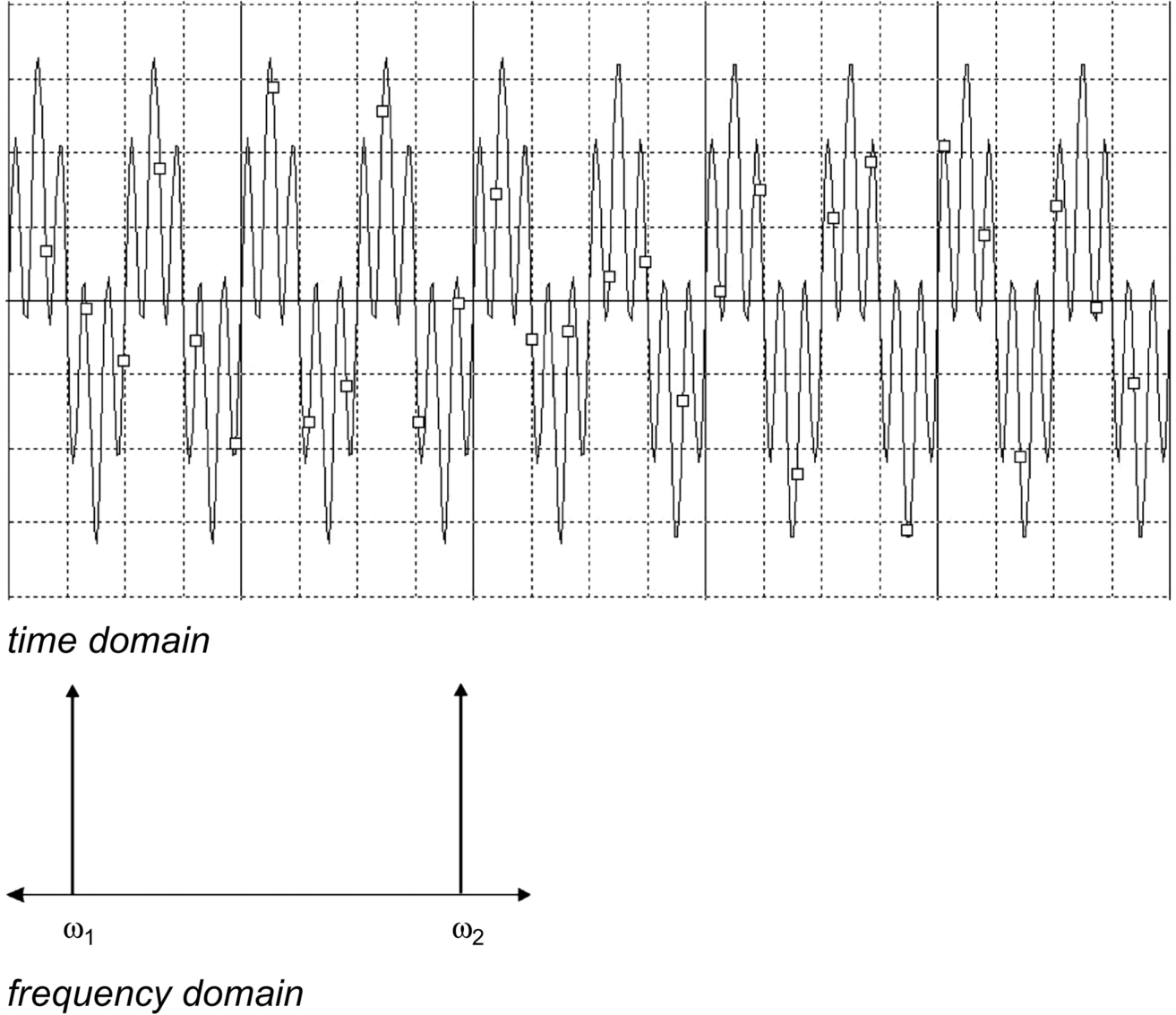
Digital circuit designers rely almost exclusively on time-domain techniques—the nonlinear nature of digital circuits is not well suited to time-domain analysis. In contrast, linear circuits use both frequency-domain and time-domain methods; frequency-domain analysis is particularly useful for many aspects of linear circuit design. Fig. 1.2 shows examples of time and frequency representations of a simple signal.
We can refer to frequencies in either of two units: the variable ω is used for radians/s; the variable f is used for Hertz. By definition, 1 Hz = 2π rad/s.
Signals can traverse large dynamic ranges that result in some very large numbers. We can reduce the magnitude of our values by using decibels (dB). This unit is one-tenth of a Bel, a unit of power named after Alexander Graham Bell. We can use decibels to express either ratios of values or to express a value relative to some reference. Since decibels refer to power, we should refer to voltage ratios as dBV although we often revert to using dB for these values as an abuse of notation.
Decibel curves are used to describe the response of filters and amplifiers. One common specification is the half-power point, also known as the 3 dB point or the corner frequency, as shown in Fig. 1.3. The plot shows power as a function of frequency. The Bode plot method allows us to approximate frequency response curves using their asymptotes. The curve is defined by two asymptotes: a flat line to the left and a line descending at 20 dB per decade to the right; that rate is equal to 6 dB per octave. The point on the curve that is 3 dB below the left-hand asymptote has a power value 1/2 that of the asymptote. Since power is related to the square of voltage, the corresponding voltage has dropped by ![]() . We often refer to the half-power frequency as the corner frequency. We will discuss Bode plots in more detail in Section 5.4.
. We often refer to the half-power frequency as the corner frequency. We will discuss Bode plots in more detail in Section 5.4.

1.5 Resistive Circuits
Electricity is a fundamental physical phenomenon. Electrical engineering (EE) is the study of techniques for the control of electricity (and, to some extent, magnetism).
EE is principally concerned with two physical quantities:
- • Electrical current, commonly represented by the variable I.
- • Electrical potential, also known as voltage, and represented by the variable V (or sometimes E for electromotive force or EMF).
Current is the macroscopic manifestation of the movement of electrons under the influence of an electrical potential. Electrons are always moving but, in isolation, their net movement is zero. An EMF results in a net movement of electrons which we can measure as current.
Ohm's law is one of the basic laws of electrical engineering:
The voltage across a device or region is proportional to the current flow through that device and its resistance R. The value of resistance is given in units of Ohms (Ω).
We sometimes prefer to work with conductance G:
Conductance is given in units Siemens S.
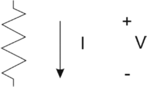
Fig. 1.4 shows the voltage across and current through a resistor. Given Ohm's law, if we know the values of two of the system parameters {I, V, R} we can determine the third.
Two other laws describe the relationship between voltages and currents when we connect several resistors into networks. Kirchoff's voltage law (KVL) says that the sum of voltages around a loop is zero:
Kirchoff's current law (KCL) states that the sum of currents into a node is zero:
Fig. 1.5 gives an example circuit in the form of a graph: the nodes {1, 2, 3} represent the points at which we evaluate Kirchoff's current law; the edges {12,13,23} are where we evaluate Kirchoff's voltage law. We can define voltage variables along the edges and currents into or out of the nodes. When we make these labels, we choose which side or direction is positive and which is negative. So long as we are consistent in our labeling, the choice doesn’t matter. The figure shows two polarities for the currents: I13 = − I31 with the subscript gives the source and sink node for the current. In practice, we often choose a polarity for each current and give it a single subscript; we use the double-subscript notation here to emphasize the source and sink nodes for each current. We could also define reverse-polarity voltages across the resistors.
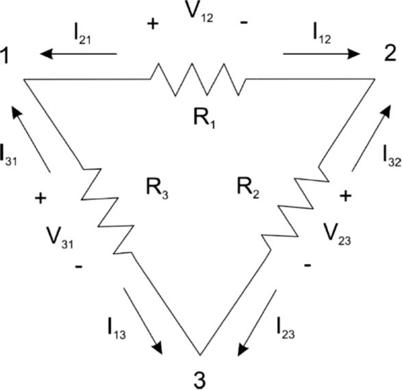
The voltages around the loop {V12, V23, V32} always sum to zero according to KVL. For any closed path through the circuit that does not repeat any circuit elements, ∑ Vij = 0.
The currents into each node always sum to zero thanks to KCL: for example, I21 + I31 = 0. When comparing the KCL equations for different nodes, we must be sure that the polarities are consistent between the nodes. Given a consistent labeling, we know that ∑ Iij = 0 for all the nodes in the circuit.
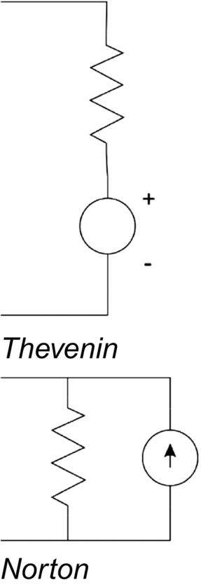
Thevenin's theorem of equivalence tells us that, given two nodes for which we can identify a voltage and current, we can find an equivalent network looking into those two nodes that consists of a voltage source in series with a resistor. In the example of Fig. 1.6, we can find the equivalent resistance of this network of three resistors. We first make use of the parallel equivalence theorem to reduce the parallel combination R2, R3:


We then use the series equivalence theorem to reduce the series combination R1, R23:
The value R123 is the Thevenin equivalent resistance. Norton's theorem of equivalence provides the current source equivalent formulation of this transformation: a voltage source and resistor network can be represented as an ideal current source in parallel with a resistor. Fig. 1.7 shows the forms of the Thevenin and Norton equivalents.
1.6 Capacitive and Inductive Circuits
Capacitors and inductors are the other two basic electrical components. They share the common characteristic that their behavior depends on the frequency of the signal applied to them.
The current through a capacitor depends on the derivative of the voltage across the capacitor C:

Fig. 1.8 shows the current through and the voltage across a capacitor. At DC, ![]() and no current flows—we say that the capacitor is an open circuit at DC. At infinitely high changes in voltage, the current through the capacitor is unlimited—it is a short circuit at high frequencies.
and no current flows—we say that the capacitor is an open circuit at DC. At infinitely high changes in voltage, the current through the capacitor is unlimited—it is a short circuit at high frequencies.

The behavior of an inductor is complementary: its voltage depends on the derivative of the current through the inductor L:

Fig. 1.9 shows the current through and voltage across an inductor. The inductor is a short circuit at DC and an open circuit at high frequencies.

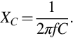
We can relate the behavior of these components more directly to a resistor by describing each as a reactance X which is a function of frequency ω, in units r/s (radians per second). The capacitor's reactance decreases with frequency:

Since ω = 2πf, we can write this as
The inductor's reactance increases with frequency:
or, in terms of Hertz,
We use units of Ohms for reactance.
As will see shortly, we can create a uniform representation for both resistance and reactance known as impedance Z or its inverse, admittance Y.
1.7 Circuit Analysis
Impedance elements are linear—their behavior can be represented in the form y = mx. The graph of this function is a line through the origin with slope m. Although lines in general do not have to go through the origin, that property is critical to the notion of linearity in physical systems. We have also assumed that our circuits are time-invariant—the signals vary with time but not the component values. Systems that are linear time-invariant (LTI) obey superposition: their response to an input which is a sum of other inputs is the sum of the responses to the individual input components.
We have seen that we can write a set of equations for the voltages and currents in a circuit and solve for the unknowns. The form of the equations depends on the structure of the circuit and on the values of its components. When solving by hand, we generally use standard algebraic methods to manipulate and reduce the equations.
A more general approach is based on linear algebra. The nodal analysis method (also known as the branch current method) is particularly well suited to solution by a computer. It writes the branch currents in terms of the node voltages and the admittances of the devices:

Given the voltages, we can solve for the currents. For a purely resistive circuit, these equations are simple. When the circuit includes reactive components, the system of equations includes differential or integral equations.
We also need more abstract representations of circuits and signals than are provided by nodal analysis and Kirchoff's laws. We can use the Laplace transform to translate the differential equations into the s domain and simplify analysis. The s parameter is complex with s = σ ± jω. (We traditionally write the imaginary number as j to avoid confusion with current.) The Laplace transform integrates with an exponential:

Many operations are easier to perform in the s domain; we can invert the transformation back into the time domain when we are done. The frequency-dependence reactance formulas of Eqs. 1.11 and 1.13 are special cases of the s domain.
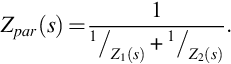
We can combine s domain impedances using the series and parallel equivalences:
We use voltage sources to describe the initial condition of capacitors and current sources for the initial condition of inductors; each has its own representation in the s domain. We can solve for the variable of interest in the s domain and then use inverse transforms to translate back into the time domain. The s-domain form of impedances allows us to algebraically manipulate resistances and reactances uniformly.
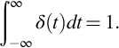
The impulse response is another key description of its behavior. An impulse δ(t) has a duration of zero time and it has unbounded value over that time; the integral of the impulse over all time is 1:
The impulse response is interesting in itself—ringing a bell is a practical example of an impulse response. But we are also interested in the impulse response because we can derive the circuit's response to other forms of input from its impulse response.
The order of a circuit or its functional model is given by the number of energy storing devices in the circuit. A first-order impulse response has the form (given here using voltage variables):
V(0) is the value of the response at t = 0 while Vf is the final value. τ is known as the time constant and is a function of the circuit components. In the case of an RC circuit, τ = RC. Fig. 1.10 shows an example of a first-order exponential response. In this case, Vf = 0; we can estimate τ from the graph by finding the time on the vertical axis at which V = V(0)e− 1 and reading off the horizontal axis value t = τ.

A second-order circuit response, illustrated in Fig. 1.11, can take one of three cases depending on the relative values of the circuit components. The overdamped case is the sum of two exponentials:

The two roots of the response s1, s2 are both real-valued, for example, s1 = 0.1 s, s2 = 0.02 s. This form of response resembles the first-order case.
The underdamped case is the sum of two damped exponentials:
The two response values are complex conjugates: s = σ ± jω. This response is very different from the first-order case—the response rises and falls around the steady-state value.
The critically damped case has the same form as the overdamped case but the two roots are identical.
1.8 Nonlinear and Active Devices
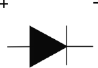
We are very interested in devices that are nonlinear: diodes, transistors, etc. The nonlinearity of diodes can be used for decisions, such as whether a given voltage represents a logic 0 or 1. Fig. 1.12 shows the schematic symbol for a standard pn diode. When a positive voltage is applied above a certain level, the current through the device is effectively that of a short circuit. When a reverse voltage is applied, the diode is effectively an open circuit. Several other types of diodes exist with specialized properties, such as operating at different voltages, emitting light, or detecting light.
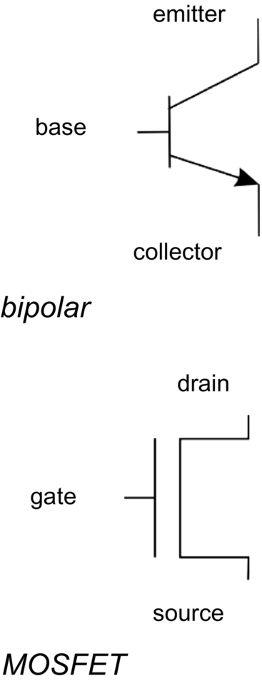
We are also extremely interested in devices—transistors, primarily—that are active. Resistors, capacitors, and inductors are all passive because they cannot amplify signals. Transistors, in contrast, provide amplification, which conveys a number of important advantages.
Fig. 1.13 shows two common transistor types. The MOSFET (metal oxide semiconductor field-effect transistor) is used for both digital and analog circuits. This symbol is for a particular type of MOSFET, enhancement mode n-type. The current between the source and drain terminals depends on the voltage at the gate. The bipolar transistor used to be widely used for both digital and analog circuits; today, it is primarily used for analog applications. The emitter-collector current is a function of the base current. In both cases, one signal can be used to control another, stronger signal. MOSFETs and bipolar transistors differ in several important ways that we will study in succeeding chapters.
Both MOSFETs and bipolar transistors can be considered at least roughly linear over a portion of their range; that linearity is used to build many types of amplifiers. However, their nonlinear characteristic cannot be ignored and they complicate the solution of the circuit equations. Circuit simulators use iterative methods to evaluate the behavior of circuits with nonlinear devices. The simulator alternates between using an estimate of the node voltages and branch currents to estimate the state of the nonlinear device, then using the device values to update the voltages and currents. Each evaluation, known as a time step, stops when the differences between successive sets of values become sufficiently small.
1.9 Design Methodologies and Tools
Ultimately, we need to move beyond circuit theory to the design of useful interfaces. A design methodology is a sequence of steps we perform during design. Some parts of the methodology will be automated while others will be manual.
We start with a set of loosely formulated requirements for the interface. We then refine those requirements into a specification that includes specific values and other details of what the interface should do.
Analysis is an important first step. We may propose some rough designs and then use our analytic tools—Kirchoff’s laws, s domain analysis, etc.—to characterize the design and to select some component values. Most of our analysis will be done by hand.
Simulation complements analysis. Simulators can analyze circuits, particularly nonlinear circuits, much more accurately than we can do by hand. Simulators can also be given a long list of input signals to help us better understand the design space. Digital logic simulation is usually done with hardware description languages (HDLs) such as Verilog or VHDL. The HDL description is fed to a simulator, which then provides waveform or tabular outputs.
The basic procedure is similar for analog circuits but with graphical input of the circuits. Fig. 1.14 shows a simple circuit for analog simulation. The circuit is entered using a schematic capture tool that is linked to a circuit simulator. We will use the OrCAD schematic capture tool and Pspice simulator throughout this book to demonstrate sample designs.

Simulating our design before we build it helps to minimize the chance of expensive and time-consuming mistakes. Some aspects of interface design are hard to simulate without expensive setups—simulating the interaction between CPU software, digital logic, and analog circuits requires a sophisticated simulator. But simulating key parts of our design using either digital or analog simulators can build confidence in the design before we buy parts and spend time building.
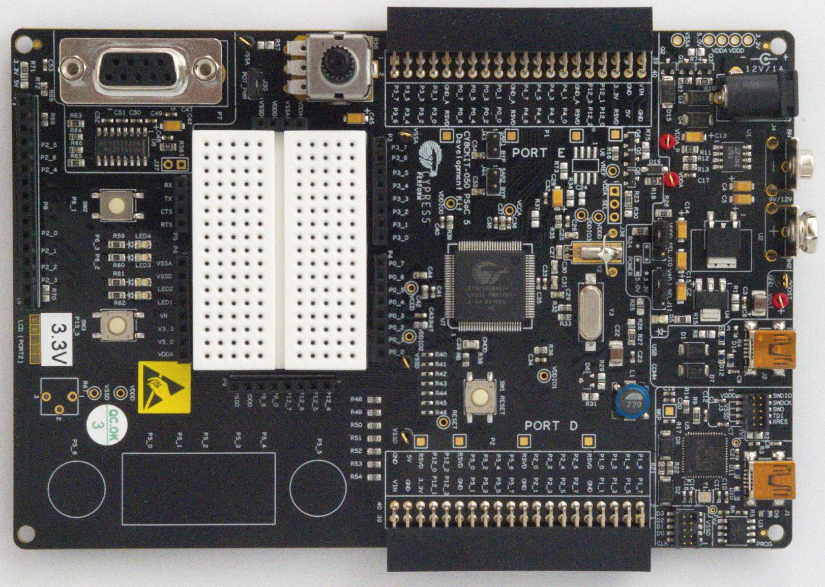
At some point, we have created our design: analog circuits, digital logic, software. Unless we are very experienced, we probably want to prototype our design to be sure it is up to snuff. Prototyping helps us ensure that the boundaries between the computer and the circuits are properly designed. Prototyping also lets us evaluate the characteristics of the circuit. While we may be able to perform simple tests of the interface without the microcontroller, we need to connect the interface to the microcontroller to fully test the system. Modern manufacturing techniques rely on advanced packages for integrated circuits that are difficult to work with manually. We typically use an evaluation board for the microcontroller we have chosen. Fig. 1.15 shows an evaluation board including a microcontroller, support logic, and switches and buttons; the rear of the board includes sockets where daughter cards can be attached. Fig. 1.16 shows an evaluation board with a prototyping module; small components can be plugged into this area, wired together, and connected to the microcontroller's inputs and outputs.

We also need some sort of equipment to test the circuit and understand what it is doing. Given the relatively slow frequencies at which many interfaces operate, relatively inexpensive equipment often works fine. A simple voltmeter allows us to test voltages around the circuit. Inexpensive oscilloscopes connect to a PC for their user interface; these instruments often include several channels of logic analyzer for digital signals.
If we only need one copy of the interface, we may be done. If we want to build multiple copies, we probably want to move beyond prototyping techniques to some form of manufacturing. Printed circuit boards (PCBs) can be manufactured in very small quantities at reasonable costs. PCBs also provide much better characteristics than do prototyping-style wiring.
Chapter 8 will also discuss prototyping and manufacturing technologies for embedded systems.
1.10 How to Read This Book
In the rest of this book, we will develop techniques for designing interfaces: we will start with subsystems and move onto complete interfaces. The chapters combine analysis with practical examples. Here is a summary of the remaining chapters:
- • Chapter 2 studies several types of standard interfaces. Many common interfaces, such as I2C or USB, are based on defined, published standards and have many commercial embodiments. Understanding how they work can help us to understand the role of interfaces in embedded systems as well as provide practical techniques.
- • Chapter 3 concentrates on digital logic interfaces. We will look at both the logical design of basic interfaces as well as their circuit characteristics. When designing logic in an FPGA, for example, we can often ignore circuit issues because our primitives are designed to be compatible. Compatibility is not assured when we mix and match logic from several different sources or when we connect analog and digital circuits. When designing interfaces, we have to be sure that our digital logic obeys basic circuit principles—if not, the interface may not behave in its properly logical manner.
- • Chapter 4 studies on amplification using transistors. Amplification is a key operation in all sorts of interfaces. Some basic principles will allow us to design and build amplifiers suited to our particular requirements.
- • Chapter 5 considers filtering, signal generation, and detection. Filtering is a critical complement to amplification. We can filter using both analog and digital techniques, each with its own advantages. We make use of several different types of controlled, precision waveforms: sine waves, square waves, etc. We may want to generate a signal directly for output; we may also use generated signals to control other parts of our interface. Detecting signals is a nonlinear operation that complements filtering.
- • Chapter 6 studies circuits that convert between analog and digital representations. Conversion is at the heart of interfacing. We need to understand how converters work in order to apply them properly and choose the best type for our application.
- • Chapter 7 looks at power delivery and conversion. Real circuits do not provide ideal power sources. We need to understand the limitations of realistic power circuits and their effects on both analog and digital circuits. Studying the design of power conversion circuits helps us understand what they do; in some cases, we may want to design our own as well.
- • Chapter 8 puts together these techniques to create mixed-signal systems that combine analog and digital systems. Mixed-signal design is the heart of interfacing. It requires us to deploy all of our design skills, both analog and digital.
The body of the book emphasizes MOSFETs. Two appendices concentrate on bipolar devices and circuits:
- • Appendix A describes TTL logic.
- • Appendix B analyzes bipolar amplifiers.
Please don’t limit your reading of this book to these pages. The book Web site contains additional material. A set of presentations summarizes the material in this book. Lab exercises complement and extend the descriptions in this text. Lab procedures can change, particularly where software is involved; the Web site provides a forum for sharing updated materials.
Questions

- Q1.2 Find an equivalent impedance for each circuit:

- Q1.3 This circuit is known as a voltage divider:

What is the ratio ![]() given R1, R2?
given R1, R2?
- Q1.4 You are given this bridge circuit:

Find Vout as a function of Vin.
- Q1.5 Plot the reactance of a capacitor with C = 1 μF over the range [628,6.28 × 106] r/s.
- Q1.6 Plot the reactance of an inductor with L = 1 mH over the range [628,6.28 × 106] r/s.
- Q1.7 Plot the impedance of these circuits over a range [20, 20 × 106] Hz:
- (a) Series R = 1 kΩ, C = 1 μF
- (b) Series L = 1 mH, C = 1 μF
- (c) Series R = 1 kΩ, L = 1 mH, C = 1 μF
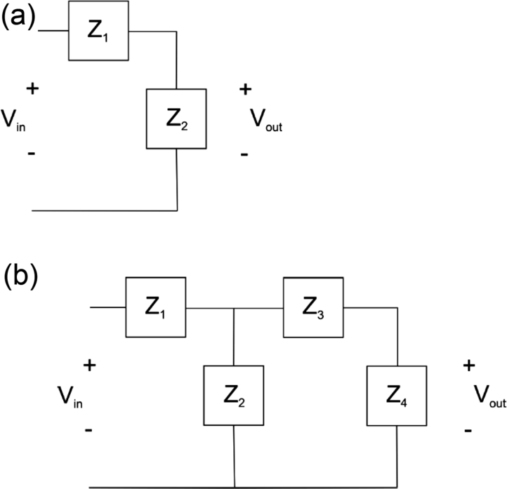
- Q1.8 For each of these ladder circuits, find the s-domain transfer function
 in terms of the Z impedances:
- Q1.9 For each transfer function, draw a pole-zero diagram:
- (a)

- (b)
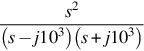
- (a)