Electric energy processing involves conversion, transfer, transmission, control, and storage of energy. Sources of energy can be converted into many forms (such as chemical, mechanical, electrical, sunlight, and wind, and audio, visual, or otherwise) including data processing by computer. This energy when transformed can be transferred and distributed. Potential energy resulting from rainfall in lakes and rivers can be converted to kinetic energy of seawater and tides, which could supply 50 percent of total world energy demand. Other forms of energy exist, such as kinetic energy of wind and solar. Other forms of energy include geothermal energy and fossil fuels such as oil, coal, and gas. Mechanical to electrical energy as simplified energy processing supply chain is shown in Figure 4.1.
Figure 4.1 Electric or magnetic fields as catalysts for electro-mechanical energy conversion.
Energy sources that are transformed and transferred are sent from the source to the consumer in different forms as needed. They are easily measurable, observable, and controllable to meet industrial, commercial, and residential loads. The creative and associative voltage and current achieve the production of power transfer. For mechanical power force and velocity are associated with mechanical power. But what is the link that enables one form of power to be converted to another?
Lorentz's force equation provides the answer; it is the force experienced by an electric charge externally by applied field, electric field, and magnetic field. The vector equation is given as
(4.1)
where F is the electromagnetic force (Newton), q is the charge (Coulombs), E is the external electric field (V/m), V is the velocity of the charge (m/s), and B is the external magnetic field (Tesla).
Since motion of charge in a conductor constitutes electric current, Lorentz's equation can be written as
(4.2)
where I is the current in the conductor (amperes), and l is the effective length in meters of the conductor subjected to the magnitude of the magnetic field.
Whenever there is field acting on a charge, it is expected that energy conversion is possible. Therefore, electric and magnetic fields serve as catalysts that enable electromechanical energy conversion to take place. Without the presence of electric and magnetic fields, no electromechanical energy conversion is possible. Examples of electromechanical energy conversion devices include electric rotating machines (generator/motors), pickups, microphones, voltmeters, ammeters, wattmeters, relays, and transformers. Some of them are presented here for illustration; they all satisfy Lorentz's equation.
Finally, machine design or simply magnetic field machines (which allow conversion) is governed by physical laws of energy-conversion processing. The design must be optimized according to some criteria to enable efficiency and low cost of operation or production.
4.2 FIRST TWO MAXWELL'S LAWS
The conversion of electro-mechanical energy involves two basic empirical Maxwell's laws.
Faraday's law states that electromotive force induced in a coil of wire is proportional to the rate of change of magnetic flux linking the coil of wire.
(4.3)
(4.4)
Or by vector notation
(4.5)
Lorentz's law states that the current-carrying conductor will experience a mechanical force when placed in a magnetic field. This force is proportional to the magnitude of the current, the magnetic field, and the effective length of the conductor subjected to the magnetic field.
(4.6)
Note that Lorentz's force has direction when
(4.7)
α gives the direction of the magnetic field.
Using the right-hand rule, if ℓ conductors carry a current and are subject to a uniform magnetic field of density B (Tesla), when the conductor is arranged in perpendicular position to the direction of magnetic field,
Then, a force is produced given by
(4.8)
This direction leads to generator actions. However, reversing the direction of α using the left-hand corkscrew rule then
(4.9)
The Faraday Case
Assume
This leads to
Therefore
at maximum
(4.10)
4.3 TRANSFORMERS
A transformer is a static device that has no moving parts but allows transfer of AC power at different voltage levels. The two electric windings wrapped in a common core can be air but are usually of ferromagnetic material. The transfer is done by electromagnetic induction (Faraday's law). Transformers are grouped in different forms based on their application and use.
4.3.1 Power and Distribution Transformers
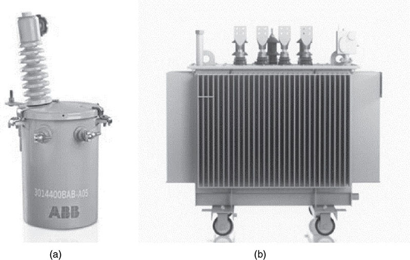
Power and distribution transformers are used primarily for transforming voltages from one level to another. Power transformers in particular are used at transmission levels to boost voltage at generation (600V–13.2 kV) to transmission voltages ranging from 132 kV to 1,000 kV and above. At the point of distribution, they are also used to step down the voltage to distribution level voltages, as seen Figure 4.2 [20].
Figure 4.2 Power and distribution transformer. Courtesy of ABB Inc.
Distribution transformers are most common at load centers. They operate at a minimum of 120/240 V (single phase/three phase) for domestic applications, while distribution voltages for commercial and industrial areas can be much higher. Distribution transformers may be mounted on plinths a little above ground level or pole mounted (see Figure 4.3 (a) and (b)) [5], [20].
Figure 4.3 Distribution transformers. (a) Pole-mounted distribution transformer (b) Ground-mounted distribution transformer. Courtesy of ABB Inc.
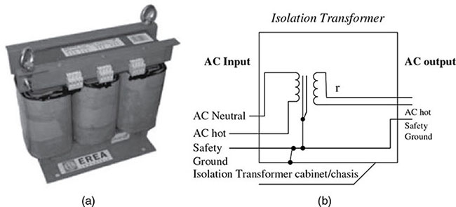
4.3.2 Isolating Transformers
Isolating transformers, as shown in Figure 4.4, [22] are used to electrically isolate electric circuits from each other or to block DC signal while maintaining AC continuity between circuits. They can also eliminate electromagnetic noise in many circuits.
Figure 4.4 (a) Physical isolating transformer. (b) Isolating system schematic. Courtesy of EREA Energy Engineering BVBV.
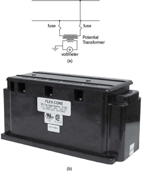
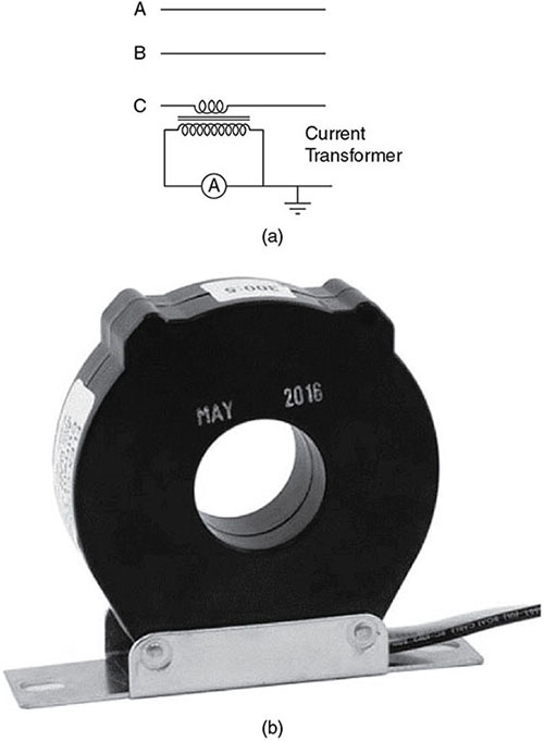
4.3.3 Instrument Transformers
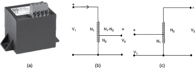
Instrument transformers are used to measure high voltages and large currents with standard small-range voltmeters, ammeters, and wattmeters, then transform voltage or current to relatively small/safe values. They are classified as potential (voltage) transformers and current transformers, and are single-phase transformers used to step down voltage or currents to safe values. Figures 4.5 and 4.6 [19] reveal the schematic diagrams and the real diagrams of instrument transformers.
Figure 4.5 (a) Schematic of a potential transformer. (b) Three-phase physical voltage transformer. Courtesy of Flex-Core.
Figure 4.6 (a) Schematic of a current transformer. (b) Solid-core current transformer. Courtesy of Flex-Core.
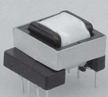
4.3.4 Communication Transformers
Communication transformers are used in electrical devices for impedance matching for improved power transfer, for isolation of DC current, and as input transformers, output transformers, and insulation apparatuses between circuits. They can be used in frequencies from 60 Hz to 400 Hz or more. In general, power transformers are designed to work at 50 Hz or 60 Hz frequencies. Transformers designed at 50 Hz or 60 Hz can be used at higher frequencies, but transformers designed at higher frequencies cannot operate at lower (50 Hz or 60 Hz) because the core would saturate and the secondary voltage would not be similar to or proportional to the primary voltage. A communication transformer is shown in Figure 4.7 [21].
Figure 4.7 Communication transformer. Courtesy of Hangzhou Smart Technology.
4.3.5 Autotransformers
The two windings of an autotransformer are not connected to each other. Hence power is transferred from one side to the other, and only by induction. There is no electrical isolation between input side and output side—so power from primary to secondary is by induction. Figure 4.8 [22] shows an autotransformer.
Figure 4.8 Autotransformer and its models. (a) Physical autotransformer (b) Step-down model (c) Step-up model. Courtesy of EREA Energy Engineering BVBV.
4.3.6 Transformer Construction and Sizes
Magnetic cores of transformers in power systems are built in core type or shell type. In either case, they are made of laminated silicon steel sheets to minimize eddy-current loss/core loss. Silicon contents decrease magnetic losses by 3 percent and 97 percent.
Transformers are constructed in different shapes and sizes for different purposes.
Distribution transformers include single- or three-phase transformers with ratings of 500kVA at voltage levels of 69 kV.
Power transformers are rated in MVA for high voltage and typically used for interstate power transfer.
Most transformer windings are immersed in a tank of oil for better insulation and cooling. When no ferromagnetic materials but only air is present, such transformers are called air-core transformers, have poor magnetic coupling, and are only used in electronic circuits. In this chapter, the focus is on the iron-core transformer.
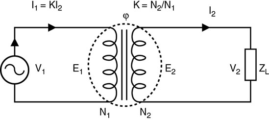
4.4 IDEAL SINGLE-PHASE TRANSFORMER MODELS
The transformer winding is modeled as the ideal case, where primary winding is referred to as NP and secondary winding as NS. From Figure 4.8, we assume:
The winding resistance is negligible.
Magnetic field intensity required to magnetize the core is negligible.
The core losses are negligible.
The magnetic flux is confined to the ferromagnetic core.
The flux generated in the core is time varying; emf e1 will be induced in a coil linking the flux. This leads to induced emf as in the primary winding N1 and induced emf e2 in the coil of secondary (N2) turns winding.
The input power in the transfer without losses is absorbed power by the losses, hence the property of the ideal transformer is a loss-free machine. If a voltage V1 is applied to the terminals of N1 turns winding, as shown in Figure 4.9, a magnetizing current will flow, producing a flux ϕ and flux linkage λ in the winding.
This equation provides a ratio of instantaneous values of induced voltages as a function of the turn ratio is a constant.
Suppose the load circuit is now connected to secondary N2 winding, causing current i2 to flow to a sink. Also, consider the flux path around the core. Flux around the closed path must be zero, therefore we can write
(4.16)
Thus, the current ratio is
(4.17)
The last equation for the current ratio is written
with the product
(4.18)
This confirms the loss-free ideal transformer, where the power input equals the power output at all instances of time. This is called the power invariance principle that means VA is conserved.
Option 1
Given the turn ratio
(4.19)
and
(4.20)
Then
(4.21)
Similarly,
(4.22)
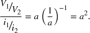
If V2 is load voltage, I2 is load current.
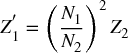
So, the ideal transformer connected to the terminals of windings of 2 to the load impedance Zin of the source will see a2Zload. That means we have transferred the load impedance from the secondary-winding side of the transformer to the primary winding side.
Example
A power of 10 kW is to be supplied to an electric furnace at a voltage 50/230 V, 60 Hz.
Compute the turn ratio.
Determine the primary and secondary currents.
Determine the impedance by 230 V supply.
Turn ratio
Secondary current
load
equating
4.5 MODELING A TRANSFORMER INTO EQUIVALENT CIRCUITS
An ideal transformer does not account for the actual practical behavior of a transformer. To include the effects of imperfection, a more accurate model of the equivalent circuit is needed. The circuit equivalent must include:
Winding resistance. For both the primary and secondary resistance, typically the winding resistance is maintained at about 0.1 percent of the terminal voltage of large transformers.
Magnetizing inductance. To account for core material used in designing the transformer, the permeability μr of the material must be determined. The value allows us to determine the flux such that N1ϕ = λ, which are the flux linkages in the transformer's magnetic property. Given the cross-sectional area of the core, the core density is given by
(4.23)
The corresponding field intensity H around the core path length is given as
(4.24)
So, the model of magnetizing current iim must flow in N1 and then by Ampère's circuital law
(4.25)
Therefore, for mostly
(4.26)
for secondary side
hence,
(4.27)
Again, magnetizing current is small in many transformers and may be specified as determined from a series of tests.
4.5.1 Modeling of Transformer Losses
The transformer core is made from ferromagnetic materials so it suffers the same problem of magnetic losses, such as eddy and hysteresis losses. They are expressed based on an empirical formula for core losses as
(4.28)
In terms of induced voltage
(4.29)
which gives:
(4.30)
where A is the area, l is the length, ρc is the core loss density.
(4.31)
where , which can also be determined experimentally.
Since core loss is small for most transformers it is negligible. But to compute the actual transformer efficiency and temperature we need to include all the losses.
4.5.2 Transformer-Equivalent Circuits
We can take advantage of the turn ratios to refer the parameters of a transformer from the secondary side to the primary side and vice versa without showing the ideal transformer.
Alternative 1: Referred to Primary Side
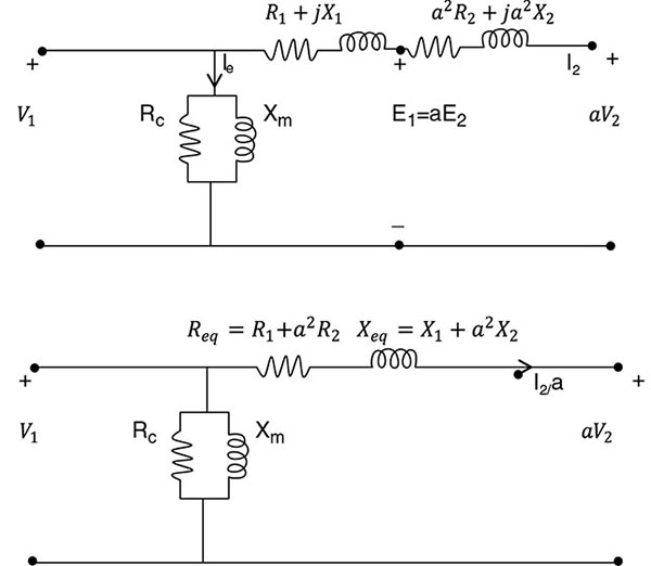
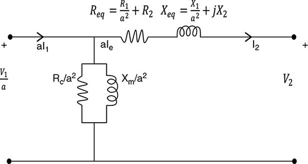
Figure 4.12 shows the final approximate equivalent circuit of a transformer referred to primary side neglecting shunt branch and winding resistance. Firstly, on Figure 4.10, the approximate equivalent circuit of a real transformer referred to primary side is given. Secondly Figure 4.11 shows the approximation when shunt branch is neglected.
Figure 4.10 Approximate equivalent circuit of real transformer (parameters referred to primary side).
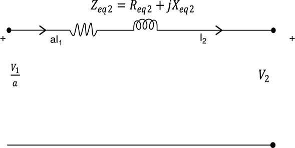
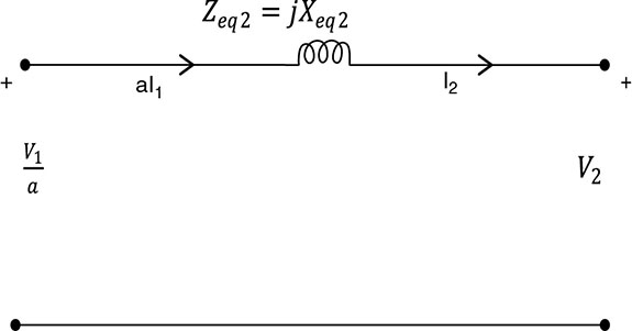
Figure 4.11 Final approximate equivalent circuit referred to the primary neglecting shunt branch.
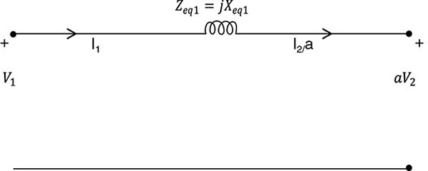
Figure 4.12 Final approximate equivalent circuit referred to the primary neglecting shunt branch and winding resistance.
The final approximate equivalent circuit neglects the transformer resistance and the shunt arm parameters since their effect in real transformer operation is negligible.
Alternative 2: Referred to Secondary Side
Alternatively, we may refer to parameters of transformer to the secondary side, as seen on Figure 4.13. The approximate equivalent circuit of the transformer is shown in Figure 4.14, which uses an equivalent impedance. Combining the secondary resistance and inductance with the primary resistance and inductance referred to the secondary and writing the resistances and reactances in terms of overall equivalent quantities, we have the equivalent impedance approximation.
Figure 4.13 Approximate equivalent circuit of real transformer with parameters referred to the secondary side.
Figure 4.14 Approximate equivalent circuit of real transformer (parameters referred to the secondary side).
Further, neglecting shunt branch will give Figure 4.15. Finally, approximate equivalent circuit when resistance is neglected will result, Figure 4.16.
Figure 4.15 Final approximate equivalent circuit referred to the secondary, neglecting shunt branch.
Figure 4.16 Final approximate equivalent circuit referred to the primary neglecting shunt branch and winding resistance.
Writing the summary of the equivalent circuit, if the transformation ratio is
R1, R2, X1, and X2 are the primary and secondary resistance and reactance, respectively.
Primary resistance referred to the secondary is
(4.32)
Overall resistance and reactance on the secondary side is
(4.33)
(4.34)
Referring secondary parameters to primary side is
(4.35)
Overall resistance and reactance on the primary side is
(4.36)
(4.37)
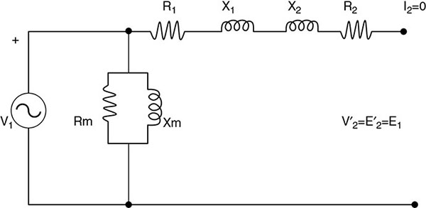
4.5.3 Determination of Equivalent-Circuit Parameters
The parameters of transformers that make up the model in Section 4.4.2 consist of R1, R2, X1, X2, Gm, and Bm. X1 and X2 are the leakage reactance, which accounts for magnetic flux that does not couple all turns. Xm is associated with mutual flux of the two windings and the resistance Rc accounts for losses due to hysteresis and eddy current. By performing two tests (open circuit and short circuit), given the transformer voltage and power rating, we can determine the values of theses parameters under loading conditions.
4.6 TRANSFORMER TESTING
Transformer testing comprises the open-circuit and short-circuit tests.
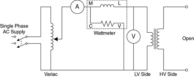
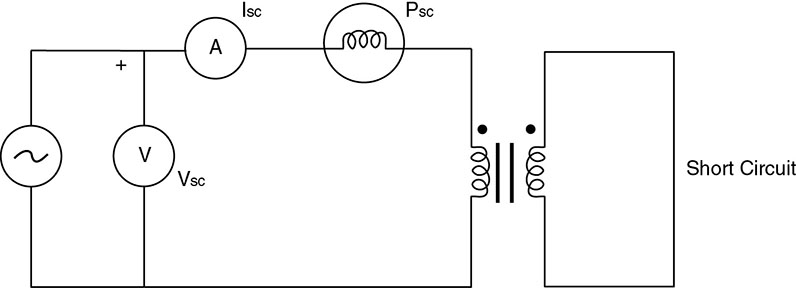
The short-circuit test is called the copper loss test and helps determine the series parameters of the primary and secondary winding model. Short circuiting one winding performs the test; typically, the primary winding is energized while the secondary winding is short circuited. Assuming the core losses are ignored and Psc = P at short circuit, the power measured by the wattmeter is the copper loss Pcu. The set-up for conducting the test is shown in Figure 4.20.
Wattmeter reads the transformer copper loss Psc = VscIsccosθsc.
Compute power factor θsc using Psc, Vsc and Isc
Note that θsc is always lagging, so always append the negative sign.
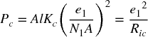
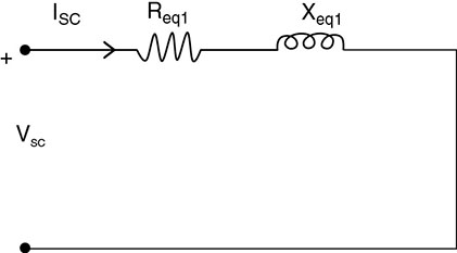
Compute the equivalent impedance of the transformer referred to the primary side Zeq1 using, Vsc, Isc, and θsc (note that Zeq1 is a complex quantity whose real and imaginary parts are Req1 and Xeq1, respectively).
Recall that Req1 = R1 + a2R2, where R1 and R2 are the primary and secondary resistances, respectively.
Also, Xeq1 = X1 + a2X2, where X1 and X2 are the primary and secondary reactances, respectively
Note that if R2' is secondary resistance referred to the primary side,
In the same vein,
Note that a is the transformation ratio.
Example
A 200/1,000 V, 50 Hz, single-phase transformer gave the following test results:
open-circuit test (LV/primary side): 200 V, 1.2A, 90 W
short-circuit test (HV/secondary side): 50 V, 5A, 110 W
Calculate the parameters of the equivalent circuit referred to the LV side.
Solution:
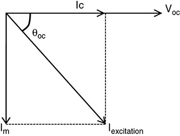
Shunt branch parameters from the open-circuit test: We need
Since the short-circuit test has been conducted from the HV side, the parameters will be computed on the secondary/HV side and then referred to primary/LV side by appropriately transforming them.
From the short-circuit test readings,
Referring these to the LV/primary side using the turns ratio
Equivalent circuits can be drawn with
Rc and Xm calculated from above and Req1 and Xeq1 as above.
4.7 TRANSFORMER SPECIFICATIONS
The information on a transformer's nameplate (as seen Figure 4.23) includes:
kVA/MVA rating
voltage rating
impedance
turn ratio
input kVA (slightly less than output kVA)
possibly a figure of merit in percent, which provides the transformer impedance
sometimes an excitation current
manufacturer and serial number
Figure 4.23 Typical transformer nameplate showing its parameters.
Other types of transformers include:
autotransformer
phase-shifter transformer
on-load tap changer (OLTC)
4.8 THREE-PHASE POWER TRANSFORMERS
Since the generated power is mostly three phase and transmitted also as three phases, the transfers are also so used. A three-phase transformer connection is necessary to step up or step down voltage levels at different source locations. The three-phase transformer is built for each phase of the primary and secondary winding associated with it. The following configurations are possible:
Y: Y
Δ: Δ
Y: Δ
Δ: Y
Each of these is described in Table 4.3, including some of the challenges or regulations required.
TABLE 4.3Three-Phase Power Transformer Configuration
4.9 NEW ADVANCES IN TRANSFORMER TECHNOLOGY: SOLID-STATE TRANSFORMERS — AN INTRODUCTION
Transformers are indispensable components of electric power systems. They are rugged and have an average efficiency of about 97.5 percent. However, they possess some undesirable properties, including sensitivity to harmonics, voltage drop under load, the need for protection from system disruptions and overload, protection of the system from problems arising at or beyond the transformer, environmental concerns regarding mineral oil, and performance under DC-offset-load unbalances. Consequently, research has been focused recently on ways overcome such concerns. With the advancement of power-electronic circuits and devices, the all-solid-state transformer is a viable option to replace conventional copper- and iron-based transformers for better power quality.
Solid-state transformers (SSTs) are a collection of high-powered semiconductor components, conventional high-frequency transformers, and control circuitry used to provide a high level of flexible control to power-distribution networks, thereby facilitating the smooth conversion of AC to DC and DC to AC as required. Add some communication capability and the entire package is often referred to as a smart transformer.
The basic structure of an SST is depicted in Figure 4.24. The isolation is achieved through a high-frequency (HF) transformer. The grid voltage is converted into HF AC voltage through power-electronics-based converters before being applied to the primary side of the HF transformer. The opposite process is performed on the HF transformer's secondary side to obtain an AC and/or DC voltage for the load.
The DC link of the third configuration is not appropriate for distributed energy resources (DER) integration since it is high voltage and has no isolation from the grid; therefore, topologies under that classification are not practical for SST implementation.
Advantages of the SST
Apart from the fact that it can step up or step down AC voltage levels, the SST has the following advantageous functionalities:
allows two-way power flow
inputs or outputs AC or DC power
actively changes power characteristics such as voltage and frequency levels
improves power quality (reactive power compensation and harmonic filtering)
provides efficient routing of electricity based on communication between utility provider, end-user site, and other transformers in the network
greatly reduces the physical size and weight of individual transformer packages with equivalent power ratings
Illustrative Problems and Examples
Problem 1
List the types of losses that occur in a transformer.
Solution:
The losses that occur in transformer are:
core losses: hysteresis loss and eddy-current loss
copper or ohmic losses
stray losses
What problems are associated with the Y–Y phase transformer connection?
Solution:
Problems associated with the Y–Y phase transformer connection include:
third harmonic component of each phase will be in phase with each other, adding up and becoming large
voltage drop at unbalanced load
over excitation in fault condition
neutral shifting
over voltage at light loads
Can a 60 Hz transformer be operated on a 50 Hz system? What actions are necessary to enable this operation?
Solution:
A 60 GHz transformer cannot be operated on a 50 Hz system. To enable this operation, a current limiter device (inductor or resistor) should be installed in series with the windings so that impedance can be increased to reduce the extra current.
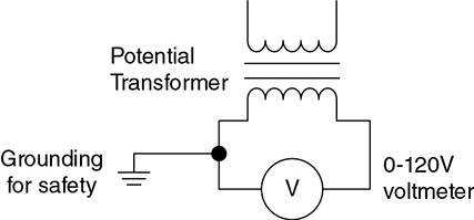
What is a potential transformer? How is it used?
Solution:
A potential transformer (as seen in Figure P1) is an instrument transformer used to measure high voltages with a standard, small-range voltmeter, which transforms the voltage to relatively small or safe values for metering. They are single-phase transformers used to step down voltages to safe (metering) values.
A 60 Hz, 120/24 V, single-phase ideal transformer has 300 turns in its primary winding. Determine the following:
value of its primary and secondary currents
number of turns in its primary windings
maximum flux Φm in the core
Solution:
We need more parameters to determine particular values of the currents. In terms of NS and NP,
Therefore,
NP= 300, NS= 60
VP= 4.44 f Φ NP
So,
Problem 3
A single-phase, 2,500/250 V, ideal transformer has a load of 10 ∠40° connected to its secondary. If the primary of the transformer is connected to a 2,400 V line, determine the following:
secondary current
primary current
input impedance as seen from the line
output power of the transformer in kVA and kW
The input power of the transformer in kVA and kW
Solution:
Secondary current
Primary current
Input impedance
Sout = IsVs = 24∠ − 40 × 240 = 5, 760∠ − 40°
Hence,
Since,
Therefore,
4.10 CHAPTER SUMMARY
The chapter provided concepts of transformer modeling and control, and the general use of transformers for power-energy systems. Transformers are critical components of any electric power system for step up or step down of voltage, instrumentation, and communication. Built on the principle of electromagnetic induction—an outflow of Maxwell's equations—transformers are powerful tools in the design of controls for electric power systems, whether operating in normal or fault modes. Advances in solid-state-transformer technology are needed for smart/microgrid systems where solid-state inverters are used. Development of commercial versions are bound to enhance their application in microgrids.
Essential concepts for transformers of different applications—including large-power transformers and distributed transformers needed for relay-protection control schemes—have been presented. Principles of modeling parameters and performance measures, such as efficiency and regulation, were also presented, and several exercises were given as illustrative examples of transformer operation and design.
EXERCISES
List the types of losses that occur in a transformer.
Why does the power factor of a load affect the voltage regulation of a transformer?
What are the problems associated with the Y–Y phase transformer connection?
Can a 60 Hz transformer be operated on a 50 Hz system? What actions are necessary to enable this operation?
What is a potential transformer? How is it used?
A 100,000kVA, 230/115 kV, Δ–Δ, three-phase power transformer has a per unit resistance of 0.01 and a per unit reactance of 0.055. The excitation branch elements are RC = 1.00 per unit and Xm = 2.0 per unit.
If this transformer supplies a load of 100MVA at 0.75 power factor lagging, draw the phasor diagram of one of the transformers.
What is the voltage regulation of the transformer bank under these conditions?
Sketch the equivalent circuit referred to the low-voltage side of one phase of this transformer.
Calculate the entire transformer impedances referred to the low-voltage side.
The results of tests on a single-phase, 10kVA, 480/120 V, 60 Hz distribution transformer are as shown in Table Q3.
Find the equivalent circuit of this transformer referred to the low-voltage side of the transformer.
Find the transformer's voltage regulation at rated conditions, with 0.8 power factor lagging and 0.8 power factor leading.
Determine the transformer's efficiency at rated conditions and 0.8 power factor lagging.
How does the efficiency of the transformer at rated conditions and 60 Hz compare to the same physical device running at 50Hz?
A single-phase 2,500/250 V, ideal transformer has a load of 10∠40° connected to its secondary. If the primary of the transformer is connected to a 2,400 V line, determine the following:
secondary current
primary current
input impedance as seen from the line
output power of the transformer in kVA and kW
input power of the transformer in kVA and kW
Assume that an ideal transformer is used to step down 13.8–2.4 kV and that it is fully loaded when it delivers 100kVA. Determine the following:
its turns ratio
rated current for each winding
load impedance referred to the high-voltage side, corresponding to full load
load impedance referred to the low-voltage side, corresponding to full load
If a 60 Hz, 120/24 V, single-phase ideal transformer has 300 turns in its primary winding, determine the following:
value of its primary and secondary currents
number of turns in its primary windings
maximum flux Φm in the core
Distinguish between a current and potential transformer.
Distinguish between a power and autotransformer.
Will a transformer designed to work in the United States at 60 Hz work in Europe/Africa, where the frequency is 50Hz?
Consider a core loss Pcore = 16 W, volt-amperes for a given core (VI)rms = 20VA, and induced voltage V = 274/ = 194Vrms when the winding has 200 turns. Find the power factor, core-loss current I c, and the magnetizing current Im.
A 15kVA, single-phase transformer with primary voltage of 2,100 V has a primary resistance of 1.0 ohm and a secondary resistance of 0.01 ohm. Find the equivalent secondary resistance and the full-load efficiency at 0.8 power factor if the iron loss of the transformer is 80 percent of full-load copper loss. Take the transformation ratio to be .
Figure Q9 shows an equivalent circuit of an ideal transformer with an impedance R2 + J X2 = 1 + j4, connected in series with the secondary. The turns ratio N1/N2 = 5:1.
Draw an equivalent circuit with the series impedance referred to the primary side.
For a primary voltage of 120 V rms and a short connected across the secondary terminals (V2 = 0), calculate the primary current and the current flowing in the short.
Figure Q9 Equivalent circuit diagram of the transformer.
The secondary winding of an ideal transformer has a terminal voltage of vs(t) = 282.8 sin 377t V. The turns ratio of the transformer is 0.5. If the secondary current of the transformer is is = 7.07 sin (377t – 36.87°) A, what is the primary current of this transformer? What are the voltage regulation and efficiency? The impedances of the transformer referred to the primary side are:
A 1,000VA, 230/115 V transformer was tested to determine its equivalent circuit. The results of the tests are shown in Table Q11.
Find the equivalent circuit of this transformer referred to the low-voltage side of the transformer.
Find the transformer's voltage regulation at rated conditions and (i) 0.8 power factor lagging, (ii) 1.0 power, and (iii) 0.8 power factor leading.
Determine the transformer's efficiency at rated conditions and 0.8 power factor lagging.
A 10kVA, 480/120 V conventional transformer is to be used to supply power from a 600 V source to a 480 V load. Consider the transformer to be ideal, and assume that all insulation can handle 600 V.
Sketch the transformer connection that will do the required job.
Find the kVA rating of the transformer in the configuration.
Find the maximum primary and secondary currents under these conditions.
Consider a 25kVA, 2,400/240 V, 60 Hz transformer with Z1 = 2.533 + j2.995Ω and Z2 = (2.5333 + j2.995) × 10− 2 Ω referred to the primary and secondary sides, respectively. Find V1, aV2, I1, I2, Req1, and Xeq1.
The transformer describe in Problem 10 is connected at the receiving end of a feeder that has an impedance of 0.3 + j1.8Ω. Let the sending-end voltage magnitude of the feeder be 2,400 V. Also, there is a load connected to the secondary side of the transformer that draws rated current from the transformer at 0.85 lagging power factor.
Neglecting the excitation current of the transformer, determine the secondary-side voltage of the transformer under such conditions.
Draw the associated phasor diagram.
Consider a 75kVA 2,400/240 V, 60 Hz transformer subjected to open-circuit and short-circuit tests. The results of the tests are shown in Table Q15.
Assuming that the transformer is operated at 0.92 lagging power factor, determine the following:
equivalent impedance, resistance, and reactance of the transformer all referred to the primary side
total loss, including the copper loss and core loss at full load
efficiency of the transformer
percentage voltage regulation of the transformer
BIBLIOGRAPHY
J. Casazza and F. Delea, Understanding Electric Power Systems: An Overview of the Technology, the Marketplace, and Government Regulations, John Wiley & Sons, Hoboken, NJ, 2003.
H. Saadat, Power System Analysis, 3rd ed., PSA Publishing, 2010.
A. E. Fitzgerald, C. Kingsley, and S. D. Umans, Fitzgerald & Kingsley's Electric Machinery, 4th ed., McGraw-Hill, New York, 1983.
C. A. Gross, Power System Analysis, John Wiley & Sons, Hoboken, NJ, 1979.
S. J. Chapman, Electric Machinery Fundamentals, 5th ed., McGraw-Hill, New York, 2012.
T. Gönen, Electrical Machines with MATLAB, 2nd ed., Taylor & Francis Group, Boca Raton, FL, 2011.
W. L. Matsch and J. D. Morgan, Electromagnetics and Electromechanical Machines, 3rd ed., John Wiley & Sons, Hoboken, NJ, 1986.
M. S. Sarma, Electric Machines: Steady-State Theory and Dynamic Performance, WMC Brown Publishers, Dubuque, IA, 1985.
R. Ramshaw and R. G. van Heeswijk, Energy Conversion: Electric Motors and Generators, Saunders College Publishing, Philadelphia, 1990.
G. R. Slemon, Electric Machines and Drives, Addison-Wesley Publishing, New York, 1992.
S. Falcones, X. Mao, and R. Ayyanar, “Topology Comparison for Solid State Transformer Implementation,” IEEE PES General Meeting, July 2010.
B. L. Theraja and A. K. Theraja, A Textbook of Electrical Technology, 1st multicolour ed., S. Chand, New Delhi, 2005.
S. J. Chapman, Electric Machinery Fundamentals, 1st ed., McGraw-Hill, New York, 2001.
D. K. Rathod, “Solid State Transformer (SST): Review of Recent Developments,” Advance in Electronic and Electric Engineering 4, 1 (2014).
X. Zhang, P. Wei, W. Deng, et al., “Emerging Smart Grid Technology for Mitigating Global Warming,” Int. J. Energ. Res. 39, 13 (2015).


 P1
P1