
“Approximate” is not a pejorative word
Abstract
“Approximate” is not a pejorative word explores the use of approximations to make data analysis simpler, faster, and more adaptable. Taylor's theorem is derived and used to linearize nonlinear functions. The method is used to create small number approximations, to estimate the variance of nonlinear functions, and to solve nonlinear least squares problems. The gradient of the error is identified as the key quantity controlling the solutions and its further application to the gradient method is explored. The lookup table is introduced as an approximate method of evaluating functions of one or two variables and applied to speeding up iterative calculations. Finally, the artificial neural network is developed as an approximation technique that shares the adaptability of a lookup table while providing smoothness and enhanced flexibility. The properties of several simple network designs are illustrated and the back-propagation algorithm for training them is derived. The power of a neural network is demonstrated by predicting the nonlinear response of a river network to precipitation.
11.1 The value of approximation
As schoolchildren, we were taught to admire the exactness of mathematics. The length of the hypotenuse of a right triangle with legs of 3 and 4 m is 5 m exactly, not a little less or a little more. Archimedes's 250 B.C.E. value of 22/7 for π was merely an upper bound for the ratio of a circle's circumference to its diameter. The exact value, known to one million digits by 1973, is something different and worth striving for.
Later in life, we learned that transcribing all 10 digits off the screen of a calculator is not really necessary; 3 or 4 is sufficient for most purposes. Yet we know that we can recompute all 10, should the need arise. We also came to appreciate the value of a back-of-the-envelope calculation, where the goal is merely to estimate the correct order of magnitude of the answer. Yet we view such calculations as imperfect—a tool to guide the development of a more accurate solution.
The situation in data analysis is fundamentally different. The accuracy of a result is a combination of methodological error, meaning error associated with the underlying theory and its computation, and observational error. Once methodological error is reduced to a level well below observation error, further improvement accomplishes little. The appropriate goal is to develop a methodology with acceptably small error, not one with none.
Of course, one might decide to err on the safe side; that is, to use only exact theories and to carry out all calculations to as many significant digits as possible. Superficially, such a strategy would not seem to be a bad one and, indeed, solutions achieved this way are certainly no worse than those that employ approximations. Yet the approach has serious limitations, over and above the obvious one that exact theories are unavailable for many imperfectly understood real-world phenomena. Approximations can bring simplicity, speed of computation, and adaptability to a solution which, in its exact form, is inscrutable, slow, and inflexible.
A simple method is one whose structure is sufficiently well-understood that its general behavior can be anticipated and its pitfalls identified and avoided. The grid search procedure (Section 4.6) for finding the minimum error solution is simple in this sense. This exhaustive search is easy to understand (and to code) and, although not completely foolproof, fails only when the search limits have been so poorly chosen that they fail to enclose the solution or when the solution varies over scale lengths smaller than the grid spacing. Linear theories of the form ![]() are simple, too. The matrix G may be large and complicated, yet it is straightforward to create and interpret. Furthermore, its least squares solution (Section 4.7) will succeed except in cases that can be easily detected (e.g., when the matrix inverse is near-singular) and corrected (e.g., by adding prior information). As we will see below, approximations that linearize an exact nonlinear theory have wide application.
are simple, too. The matrix G may be large and complicated, yet it is straightforward to create and interpret. Furthermore, its least squares solution (Section 4.7) will succeed except in cases that can be easily detected (e.g., when the matrix inverse is near-singular) and corrected (e.g., by adding prior information). As we will see below, approximations that linearize an exact nonlinear theory have wide application.
Approximations can also improve the speed of computation. Speed is an extremely important issue in very large problems that challenge the capabilities of the current generation of computers and in real-time applications, where a solution is needed immediately after the data becomes available. A Global Positioning System (GPS) receiver would be of limited utility in an automobile if it took 10 min to determine a location!
Finally, some data analysis scenarios need to adapt to evolving conditions that affect the character of the data. The character of a river hydrograph, for example, may evolve significantly over the years as its watershed becomes urbanized. The methodology needed to predict discharge from precipitation may need to be correspondingly updated. Some approximate methods are particularly well-suited for incorporating machine learning.
11.2 Polynomial approximations and Taylor series
A polynomial can always be designed to behave similarly to a smooth function y(t) in the vicinity of a specified point t0. This assertion can be demonstrated by constructing a polynomial yp(t) that has the same value, first derivative, second derivative, etc. at this point. The polynomial becomes a better and better approximation to the function as derivatives of higher and higher order are matched (Figure 11.1). A polynomial with unknown coefficients ci is
and its derivates are


 (gray curve) approximated by a sequence of polynomials of increasing degree. Note that the approximations become more accurate, especially near the point t0, as the degree is increased. MatLab script eda11_01.
When evaluated at the point ![]() , these functions each depends upon a single constant:
, these functions each depends upon a single constant:

After solving for the constants and inserting them into Equation (11.1), a polynomial yp(t) is obtained, whose value and derivatives match the smooth function y(t) at the point t0:

This polynomial can be shown to converge to the smooth function when the number of terms becomes indefinitely large; that is, ![]() (at least for a finite interval of the t axis containing t0). This result is known as Taylor theorem and Equation (11.4) is known as the Taylor series representation of the function y(t). As we will show below, Taylor series play a critical role in many approximation methods.
(at least for a finite interval of the t axis containing t0). This result is known as Taylor theorem and Equation (11.4) is known as the Taylor series representation of the function y(t). As we will show below, Taylor series play a critical role in many approximation methods.
11.3 Small number approximations
An important class of approximations uses just the first two terms of the Taylor series to represent a function in the neighborhood of a point ![]() , since the higher order terms are typically negligible there. Consider the function
, since the higher order terms are typically negligible there. Consider the function ![]() . At the point
. At the point ![]() , it has value
, it has value ![]() and first derivative
and first derivative ![]() . Inserting these values into Equation (11.4) yields
. Inserting these values into Equation (11.4) yields
This approximation is surprisingly accurate. For instance, ![]() , whereas
, whereas ![]() ; the difference is only 0.02 %.
; the difference is only 0.02 %.
Two additional examples are the functions sin t and cos t in the neighborhood of the point ![]() . The sine has a value of 0, a first derivative of 1, and a second derivative of 0 at this point, while the cosine has a value of 1, a first derivative of 0, and a second derivative of
. The sine has a value of 0, a first derivative of 1, and a second derivative of 0 at this point, while the cosine has a value of 1, a first derivative of 0, and a second derivative of ![]() there. Inserting these values into Equation (11.4) yields
there. Inserting these values into Equation (11.4) yields
These and other small number approximations can be used to simplify and speed up data analysis problems (see Crib Sheet 11.1).
11.4 Small number approximation applied to distance on a sphere
A common problem encountered when working with geographical data is to determine the great circle distance r between two points on a sphere (such as the Earth). Spherical trigonometry can be used to show that this distance, measured in degrees of arc, is given by
Here, λ1 and λ2 are the latitudes of the two points, respectively; L1 and L2 are their longitudes; and ![]() . Six distinct trigonometric functions must be evaluated in order to determine r—a time-consuming process. A small r approximation can reduce the count of functions. The first step is to define the difference in latitude as
. Six distinct trigonometric functions must be evaluated in order to determine r—a time-consuming process. A small r approximation can reduce the count of functions. The first step is to define the difference in latitude as ![]() and the mean latitude as
and the mean latitude as ![]() . Standard trigonometric identities are then used to rewrite Equation (11.7) in terms of these quantities:
. Standard trigonometric identities are then used to rewrite Equation (11.7) in terms of these quantities:

By assumption, ΔL, Δλ, and r are all small. After applying the small number approximations of Equation (11.6) and after considerable algebra, the approximation is found to be

The first two terms on the right-hand side represent the Euclidian distance between the points; that is, distance as measured on a plane. The last term corrects this flat-earth distance for the curvature of the surface. Only two functions, a cosine and a square root, need to be evaluated in order to determine r, which is a factor-of-three reduction in effort compared with the exact formula. Furthermore, the approximation is very accurate, at least out to distances of a few degrees (Figure 11.2).

 . MatLab script eda11_02.
11.5 Small number approximation applied to variance
A commonly encountered problem is that of estimating the variance of a nonlinear function of the model parameters. As an example, suppose that a least squares procedure estimates an angular frequency mest with variance σm2, but we would rather state confidence bounds for the period ![]() . As discussed in Chapter 3, this problem can be solved exactly by assuming that m is normally distributed, working out the probability density function p(T), and then calculating its mean and variance. However, the exact procedure is difficult and time-consuming; the approximation that is developed here is accurate when
. As discussed in Chapter 3, this problem can be solved exactly by assuming that m is normally distributed, working out the probability density function p(T), and then calculating its mean and variance. However, the exact procedure is difficult and time-consuming; the approximation that is developed here is accurate when ![]() .
.
The idea is to examine how a small fluctuation Δm in frequency causes a small fluctuation ΔT in period. Writing ![]() and
and ![]() and inserting them into the formula relating frequency and period yield
and inserting them into the formula relating frequency and period yield

After equating Test with 2π/mest, small fluctuations in period and frequency are found to be related through

If the fluctuations in Δm have a variance of σm2, then according to the usual rules of error propagation, the fluctuations in ΔT will have variance:

The period T has the same variance, since it differs from ΔT only by an additive constant. As an example, we consider the case ![]() rad/s,
rad/s, ![]() rad/s, which leads to
rad/s, which leads to ![]() s and
s and ![]() s, estimates that agree well with a numerical simulation (Figure 11.3).
s, estimates that agree well with a numerical simulation (Figure 11.3).

 and variance
  (gray curve). An empirical probability density function (dashed curve) based on a histogram of 10,000 realizations of mi closely matches this function. (B) Normal probability density function p(T) for period
  , with mean
  and variance σT2 calculated using the linear approximation discussed in the text (gray curve). An empirical probability density function (dashed curve) based on a histogram of
  closely matches this function. MatLab script eda11_03.
11.6 Taylor series in multiple dimensions
In a typical data analysis problem, the predicted data dpre(m) is a function of model parameters m. The Taylor series for dpre(m) is a straightforward generalization of the one-dimensional series and can be shown to be

The sequence of terms is the same as in the one-dimensional case: a constant term; a linear term, a quadratic term, and so forth. Derivatives of the same order appear in the same places in both formulas, as well: the linear term is multiplied by a first derivative; the quadratic term by a second derivative; and so forth. The main complication is that both the data and the model parameters are subscripted quantities, so summations are involved. Note that the first derivative has two subscripts and is therefore a matrix, say G(0):
The matrix G is called the linearized data kernel. The Taylor series is a little simpler when a scalar function of the model parameters, such as the prediction error E, is being considered:

The first derivative has one subscript and so is a vector, say b(0), and the second derivative has two subscripts and so is a matrix, say B(0):

The quantities b and B are called the gradient vector and the curvature matrix, respectively. Equations (11.13) and (11.15) can then be written in vector notation as

11.7 Small number approximation applied to covariance
The procedure for estimating variance (Section 11.5) can be generalized to the nonlinear vector function T(m), providing a way to estimate the covariance matrix CT. The first step is to expand the function T(m) in a Taylor series around the point mest and keep only the first two terms. The resulting linear approximation relates small fluctuations in m to small fluctuations in T:

The standard error propagation rule (Section 3.12) then gives ![]() .
.
11.8 Solving nonlinear problems with iterative least squares
The error E(m) and its derivatives can be computed as long as the theory dpre(m) is known, irrespective of whether it is linear or nonlinear. Consequently, we can apply the principle of least square to nonlinear problems; the solution mest is the one that minimizes the error E(m), or equivalently, the one that solves ![]() . Unfortunately, this set of nonlinear equations is usually difficult to solve exactly. However, if we can guess a trial solution m0 that is close to the minimum error solution, then we can use Taylor's theorem to approximate E(m) as a low order polynomial centered about this point. If m0 is close enough to the minimum that a quadratic approximation will suffice, then the process of solving
. Unfortunately, this set of nonlinear equations is usually difficult to solve exactly. However, if we can guess a trial solution m0 that is close to the minimum error solution, then we can use Taylor's theorem to approximate E(m) as a low order polynomial centered about this point. If m0 is close enough to the minimum that a quadratic approximation will suffice, then the process of solving ![]() is very simple, because the derivative of a quadratic function is a linear function. Differentiating the expression for E in Equation (11.17) and setting the result to zero yield
is very simple, because the derivative of a quadratic function is a linear function. Differentiating the expression for E in Equation (11.17) and setting the result to zero yield
This equation enables us to find an updated solution, ![]() , that is closer to the minimum than is m0. This process can be iterated indefinitely, to provide a sequence of ms that, under favorable circumstances, will converge to the minimum error solution. It is sometimes referred to as Newton's method. A limitation is that the curvature matrix B must be calculated, in addition to the gradient vector b. Calculating this matrix may be difficult.
, that is closer to the minimum than is m0. This process can be iterated indefinitely, to provide a sequence of ms that, under favorable circumstances, will converge to the minimum error solution. It is sometimes referred to as Newton's method. A limitation is that the curvature matrix B must be calculated, in addition to the gradient vector b. Calculating this matrix may be difficult.
In the special case of the linear theory ![]() , the error is
, the error is
The unknown quantities m0, b, and B are found by comparison with Equation (11.17):
Inserting these values into Equation (11.19) yields the familiar least squares solution: ![]() . This correspondence suggests the strategy of approximating the curvature matrix as
. This correspondence suggests the strategy of approximating the curvature matrix as ![]() , in which case the procedure for updating a trial solution m(k) is (Tarantola and Valette, 1982; see also Menke, 2014)
, in which case the procedure for updating a trial solution m(k) is (Tarantola and Valette, 1982; see also Menke, 2014)

The covariance of the solution is approximately
where kmax signifies the final iteration.
This procedure is known as iterative least squares. An important issue is when to stop iterating. Possibilities include when the error of the fit, as quantified by its posterior variance, declines below a specified value that represents the fit being acceptably good; or when the error no longer decreases significantly between iterations; that is, when ![]() declines below a specified value; or when the solution no longer changes significantly between iterations; that is {[Δm]T[Δm]}1/2 declines below a specified value.
declines below a specified value; or when the solution no longer changes significantly between iterations; that is {[Δm]T[Δm]}1/2 declines below a specified value.
Prior information, represented by the linear equation ![]() , can be added to the procedure in order to generalize it. The only nuance is that the prior information is satisfied by the model parameters
, can be added to the procedure in order to generalize it. The only nuance is that the prior information is satisfied by the model parameters ![]() and not by the model perturbation Δm. Inserting
and not by the model perturbation Δm. Inserting ![]() into the prior information equation yields
into the prior information equation yields
See Crib Sheet 11.2 for the complete formulation.


11.9 Fitting a sinusoid of unknown frequency
Suppose that the data consists of a single sinusoid superimposed on a background level, and that the amplitude, phase, and frequency of the sinusoid, as well as the background level, is unknown. This scenario is described by an equation that is nonlinear in the model parameters:
The constants ![]() , A, and ωa have been introduced in order to normalize the size of the model parameters, which will be in the
, A, and ωa have been introduced in order to normalize the size of the model parameters, which will be in the ![]() range (or close to it) when these constants are properly chosen. The matrix G(k) has elements:
range (or close to it) when these constants are properly chosen. The matrix G(k) has elements:

This model can be applied to the Black Rock Forest temperature data, which has a pronounced annual cycle. We set ![]() to the mean of the data, A to half its range, and ωa to the frequency 2π/365 rad/day. A reasonable trial solution is
to the mean of the data, A to half its range, and ωa to the frequency 2π/365 rad/day. A reasonable trial solution is ![]() . (The choice
. (The choice ![]() ,
, ![]() implies that the highest temperature is in summer.) The iterative procedure of Equation (11.22) is then used to refine this estimate. The iteration process is terminated when the change in model parameters, from one iteration to the next, drops below a predetermined value (in this example,
implies that the highest temperature is in summer.) The iterative procedure of Equation (11.22) is then used to refine this estimate. The iteration process is terminated when the change in model parameters, from one iteration to the next, drops below a predetermined value (in this example, ![]() ).
).
This method produces an estimated period of ![]() days (95%), where the confidence interval was computed by the method of Section 11.5. Whether the nonlinear fit (Figure 11.4) provides a better estimate of the period that can be determined from standard amplitude spectral density analysis is debatable. The annual peak in the amplitude spectral density is broad, owing to the relatively few annual oscillations in the temperature time series (only 11). Nevertheless, its center is very close to the value determined by the nonlinear analysis (Figure 11.5).
days (95%), where the confidence interval was computed by the method of Section 11.5. Whether the nonlinear fit (Figure 11.4) provides a better estimate of the period that can be determined from standard amplitude spectral density analysis is debatable. The annual peak in the amplitude spectral density is broad, owing to the relatively few annual oscillations in the temperature time series (only 11). Nevertheless, its center is very close to the value determined by the nonlinear analysis (Figure 11.5).


11.10 The gradient method
The gradient vector ![]() represents the slope of the error function E(m) in the vicinity of the trial solution m(k). It points in the direction in which the error most rapidly increases, which is to say, directly away from the direction in which m(k) must be perturbed to lower the error. For this reason, its appearance in the rule for updating a trial solution m(k) (Equation 11.19) is unsurprising. This relationship is further examined by rewriting the update rule as
represents the slope of the error function E(m) in the vicinity of the trial solution m(k). It points in the direction in which the error most rapidly increases, which is to say, directly away from the direction in which m(k) must be perturbed to lower the error. For this reason, its appearance in the rule for updating a trial solution m(k) (Equation 11.19) is unsurprising. This relationship is further examined by rewriting the update rule as

Here |b| is the length of b. This rule has a simple interpretation: the vector ν(k) is the downslope direction; that is, the direction in which m(k) should be perturbed to most reduce the error. The matrix M(k) encodes information about the size of the perturbation needed to reach the minimum in the error E(m), and although it also can change the direction of the perturbation, this effect is usually secondary.
The gradient vector b(k) can be computed easily from the linearized data kernel G(k):

The calculation of the matrix M(k) is more difficult because it involves taking a matrix inverse. A trial solution would be easier to update if it could be omitted from the formula. The gradient method approximates M(k) as αI, where α is an unknown step size. An initial guess for α is made at the start of the error minimization process and is used to tentatively update the trial solution according to the rule ![]() . The iteration process continues if the error
. The iteration process continues if the error ![]() has decreased. However, if the error has increased, the new solution has overshot the minimum because the step size is too big. The step size is decreased, say by replacing α with α/2, and another tentative solution is tried.
has decreased. However, if the error has increased, the new solution has overshot the minimum because the step size is too big. The step size is decreased, say by replacing α with α/2, and another tentative solution is tried.
The main limitation of the gradient method, compared to iterative least squares, is that more iteration is needed to achieve an acceptable solution. While each step moves the solution towards the minimum, the step size has not been correctly set to move it to the minimum, so convergence is much slower. When applied to Black Rock Forest temperature problem described in the previous section, about 3500 iterations of the gradient method are needed to provide an acceptable solution (Figure 11.6) whereas fewer than 10 iterations of the iterative least squares method are needed for a solution with similar accuracy.

The least squares error E(m) is the sum of many individual errors:

In many practical cases, the number of individual errors is very large (N ≈ 100,000 in the Black Rock Forest case). The updating rule ![]() is only approximate. The omission of some of the individual errors from the formula for ν(k) makes it somewhat more approximate, but as long as ν(k) is not too inaccurate, each step will still move the solution towards the minimum. Furthermore, if a different random subset of individual errors is used in each step, the entire dataset can be cycled through during the course of the solution. This approximation is called the stochastic gradient method. In the case of the Black Rock Forest dataset, a reduction of the number of individual errors by a factor of 1000 still leads to an acceptable solution (Figure 11.6).
is only approximate. The omission of some of the individual errors from the formula for ν(k) makes it somewhat more approximate, but as long as ν(k) is not too inaccurate, each step will still move the solution towards the minimum. Furthermore, if a different random subset of individual errors is used in each step, the entire dataset can be cycled through during the course of the solution. This approximation is called the stochastic gradient method. In the case of the Black Rock Forest dataset, a reduction of the number of individual errors by a factor of 1000 still leads to an acceptable solution (Figure 11.6).
11.11 Precomputation of a function and table lookups
Many data analysis methods require that the same function be evaluated numerous times. If the function is complicated but has only one or two arguments of known range, then precalculating it and storing its values in a table may prove computationally efficient. As long as the time needed to perform a table lookup is less than the time needed to evaluate the function, computation time is reduced. Some accuracy is lost, too, since a table lookup provides only an approximate value of the function, but in many cases this inaccuracy is overwhelmed by other sources of error (and especially measurement error) that enter into the problem.
The lookup table for a one-dimensional function d(x) is just the time series ![]() with
with ![]() . The range of xk must encompass all values of x that need to be estimated, and the sampling must be small enough to faithfully represent fluctuations in the function. A simple estimate of the function d(x) is the value of the corresponding table entry, dn with
. The range of xk must encompass all values of x that need to be estimated, and the sampling must be small enough to faithfully represent fluctuations in the function. A simple estimate of the function d(x) is the value of the corresponding table entry, dn with ![]() . Here the function floor(x) is the largest integer smaller than x. Alternatively, d(x) could be estimated by linearly interpolating between the two bracketing dn and
. Here the function floor(x) is the largest integer smaller than x. Alternatively, d(x) could be estimated by linearly interpolating between the two bracketing dn and ![]() , though the interpolation process adds computation time.
, though the interpolation process adds computation time.
As an example, we consider the problem of using a grid search to determine two model parameters (m1, m2) where the data di(ti) obeys
Note that di(xi) is a complicated function of just one variable xi(ti). In order to set up the lookup table, we need to know the range of plausible values of the model parameters (m1, m2) and time t. Let us suppose that they are ![]() ,
, ![]() , and
, and ![]() . These ranges allow us to compute the range for the xs in the lookup table as
. These ranges allow us to compute the range for the xs in the lookup table as ![]() . The version of the grid search that uses the lookup table executes in only about half the time of the version that directly computes di(ti) each time it is needed (Figure 11.7).
. The version of the grid search that uses the lookup table executes in only about half the time of the version that directly computes di(ti) each time it is needed (Figure 11.7).

Lookup tables are applicable to functions of two or more variables, but tables of more than two dimensions are seldom useful, because the time needed to construct them is very large.
11.12 Artificial neural networks
Suppose that the function d(x) is not accurately known. One strategy is to start with an initially poor estimate of it and improve it as new information becomes available. One advantage of using a lookup table to represent the function is that a table is easily updated. The values of its elements can be trivially changed to reflect new information. However, a table is also inflexible, in the sense that, once defined, the width Δx of its elements cannot easily be changed to reflect new information about the scale length over which d(x) varies. Furthermore, the value of d(x) jumps abruptly as an interval boundary is crossed, which may violate prior information about the function's smoothness. In this section, a new approximation, called the artificial neural network (or neural net, for short), is introduced. It shares some similarity with a lookup table but is more adaptable and smooth. (Notice that the attribute of the lookup table upon which we are focusing is updatability, not computation speed; neural nets are not especially speedy.)
An arbitrary function d(x) can be represented schematically as a row of three boxes, with interconnecting lines that represent information flowing from left to right (Figure 11.8A). In this network representation, the left box represents input x, the right box represents output d(x), and the middle box represents the workings of the function, which may be arbitrarily complicated. The middle box encapsulates (or hides) all the details of the function, and for this reason is said to be hidden. The table approximation replaces the workings in the middle box with a simple table lookup (Figure 11.8B). Since each element of the table specifies the value of the function d(x) in a distinct interval of the x-axis, the process of interrogating the table lookup can be viewed as summing boxcar or tower functions, each of which is constant in the interval and zero outside of it (Figure 11.8C).

The left and right edges of the each table entry can be made separate by viewing a tower as the sum of two step functions:
Here H(z) (with ![]() ) is the Heaviside step function, defined as zero when
) is the Heaviside step function, defined as zero when ![]() and unity when
and unity when ![]() . The weights w and the biases b parameterize the location of the edges, with the left edge at
. The weights w and the biases b parameterize the location of the edges, with the left edge at ![]() and the right edge at
and the right edge at ![]() . The constant dc specifies the height of the tower (Figure 11.9). In a lookup table, the edges of adjacent towers match one another; that is,
. The constant dc specifies the height of the tower (Figure 11.9). In a lookup table, the edges of adjacent towers match one another; that is, ![]() and
and ![]() (where the superscript consecutively numbers the towers). However, in a neural net, this requirement is relaxed and step functions are allowed to overlap in any fashion.
(where the superscript consecutively numbers the towers). However, in a neural net, this requirement is relaxed and step functions are allowed to overlap in any fashion.

The issue of smoothness is addressed by replacing the step function H(z) by the sigmoid function:

Like the step function, this function asymptotes to zero and unity, respectively, as ![]() and has a transition centered on
and has a transition centered on ![]() (or
(or ![]() ). Unlike the step function, the sigmoid function is smooth. The parameter w controls the sharpness of the transition, with a maximum slope at x0 of
). Unlike the step function, the sigmoid function is smooth. The parameter w controls the sharpness of the transition, with a maximum slope at x0 of ![]() (Figure 11.10).
(Figure 11.10).
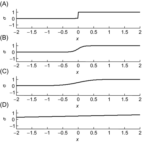
 . (A) Slope
  ,
,  . (B) Slope
  , . (C) Slope
  , . (D) Slope
  , . Note that the width of the transition is sharper for the larger ss. MatLab script eda11_08.
11.13 Information flow in a neural net
A neural net consists of L columns (or layers) of boxes, with the kth layer containing N(k) boxes. Because the neural net approximation was motivated by studies of information flow in animal brains, the boxes are called neurons. Information flows from left to right along connections, denoted by line segments connecting the boxes in adjacent layers. Neuron i in layer k has one parameter associated with it, its bias bi(k). The connection between neuron i in layer k and neuron j in layer ![]() has one parameter associated with it, its weight wij(k); the absence of a connection is indicated by a zero weight. Neuron i in layer k also has an input value zi(k) and an output value (or activity) ai(k). The activities of neurons in layer 1 represent the input to the function and the activities of the neurons in layer L represent the output of the function. In the one-dimensional case considered above, layer 1 has one neuron with activity x and layer L has one neuron with activity d(x). However, neural nets can handle a multidimensional function d(x) simply by having multiple input and output neurons. The rule for propagating information between one layer and the next is
has one parameter associated with it, its weight wij(k); the absence of a connection is indicated by a zero weight. Neuron i in layer k also has an input value zi(k) and an output value (or activity) ai(k). The activities of neurons in layer 1 represent the input to the function and the activities of the neurons in layer L represent the output of the function. In the one-dimensional case considered above, layer 1 has one neuron with activity x and layer L has one neuron with activity d(x). However, neural nets can handle a multidimensional function d(x) simply by having multiple input and output neurons. The rule for propagating information between one layer and the next is

These relationships are depicted in Figure 11.11. Once the activities in layer 1 are specified, this rule can be used to propagate information layer by layer through the neural network. A simple MatLab function that performs this operation is provided:

a = eda_net_eval(N,w,b,a);
% set the activities of the layer 1 before calling this function
% N(i): column-vector with number of neurons in each layer;
% biases: b(1:N(i),i) is a column-vector that gives the
% biases of the N(i) neurons on the i-th layer
% weights: w(1:N(i),1:N(i-1),i) is a matrix that gives the
%  weights between the N(i) neurons in the i-th layer
%  and the N(i-1) neurons on the (i-1)-th layer.
% activity: a(1:N(i),i) is a column-vector that gives the
% activities of the N(i) neurons on the i-th layer
(MatLab eda_net_eval)
The neural nets for smoothed versions of a step function and a tower function are shown in Figure 11.12. Since the sigmoid function is omitted on the output layer, the activity of this layer is just a weighted sum of its inputs. This feature allows the easy amalgamation of networks. For instance, several single-tower networks can be amalgamated to yield a sum of towers (Figure 11.13).

 ,
,  ,
,  case. (C) Graph for the , , case. (D) Neural net for a smoothed version of a tower function d(x) with amplitude A, transitions at x1 and at x2, and slope s. (E) Graph for the
  ,
,  ,
,  , case. (F) Graph for the , , , case. MatLab scripts eda11_09 and eda11_10.
A two-dimensional tower, say for input (x, y), can be created by amalgamating two one-dimensional tower networks, a tower in x and a tower in y (Figure 11.14A). However, their sum is not quite a two-dimensional tower function but rather consists of two intersecting ridges, one parallel to the x-axis and the other parallel to the y-axis, with a hump where the tower should be (Figure 11.14B). A fourth layer, implementing a step function with a transition higher than the ridges but lower than the hump, is needed to delete the ridges and form the tower (Figure 11.14C).

 and
and  . (B) The input to the third layer has low-amplitude ridges (gray) that intersect to produce a high amplitude hump (black). (C) The fourth layer deletes the ridges but leaves the hump. Its output is the tower. MatLab script eda11_12.
A function can be approximated to any degree of fidelity by summing together enough towers. Thus, a neural network is capable of approximating any continuous function. However, a network constructed in this fashion may not be the smallest capable of adequately approximating the function. In the next section we will develop a technique to train an arbitrary network to produce the best approximation of a function of which it is capable. This is a simple form of machine learning.
11.14 Training a neural net
The goal in training a neural net is to match the output ![]() of the neural net to some set of observed values (xi, diobs); that is, to find a set of weights and biases such that
of the neural net to some set of observed values (xi, diobs); that is, to find a set of weights and biases such that ![]() . This problem can be solved by defining an error
. This problem can be solved by defining an error ![]() and finding the weights and biases that minimize the total error
and finding the weights and biases that minimize the total error ![]() . Since the neural net is inherently nonlinear, the error minimization must be performed with the iterative least squares method (Section 11.8) or the gradient method (Section 11.10). The process refines an initial guess of the model parameters (the combined set of weights and biases) into a final estimate that minimizes the prediction error.
. Since the neural net is inherently nonlinear, the error minimization must be performed with the iterative least squares method (Section 11.8) or the gradient method (Section 11.10). The process refines an initial guess of the model parameters (the combined set of weights and biases) into a final estimate that minimizes the prediction error.
Both procedures require the derivatives:

At first glance, computing these derivatives appears to be a daunting task. However, recall that dipre is just the activity of neuron 1 in layer L, and the formula for computing activities (Equation 11.33) is simple and easily differentiated. The chain rule (see Note 11.1) implies

While the derivatives of Equation (11.35) are of varying complexity, they are all tractable. The easiest is

The two next most complicated are

More complicated still is

Finally, the ![]() derivative is built layer by layer, using another application of the chain rule. The derivative that connects changes in activities on adjacent layers is
derivative is built layer by layer, using another application of the chain rule. The derivative that connects changes in activities on adjacent layers is

A succession of these derivatives can be used to connect the activities on the Lth layer to all the other layers, a process called back-propagation, since it starts with the Lth layer and works backward towards the first layer (Figure 11.15) (Werbos, 1974):

The summation arises because a perturbation in the activity of a neuron on the kth layer is due to the combined effect of perturbations of the activities of all the neurons on the (k − 1)th layer that connect with it (see Note 11.1).

 , which in turn is caused by perturbations Δa1(3) and Δa2(3), which in turn are caused by perturbation Δa1(2), which in turn is caused by input perturbation Δz1(2), which in turn is caused by a perturbation Δw11(2) in a specific weight.
A MatLab function that calculates the derivatives is provided:
[daLmaxdw, daLmaxdb] = eda_net_deriv(N,w,b,a);
% update the activities by calling a=eda_net_eval(N,w,b,a);
% before calling this function
% daLmaxdb(i,j,k): the change in the activity of the i-th neuron
% in layer Lmax due to a change in the bias of the of
% the j-th neuron in the layer k
% daLmaxdw(i,j,k,l): the change in the activity of the i-th
% neuron in layer Lmax due to a change in the weight
% connecting the j-th neuron in the layer l with the k-th
% neuron of layer l-1
(MatLab eda_net_deriv)
The weights and biases together constitute the model parameters m of the iterative least squares problem (Section 11.8). The matrix Gij(p) contains the derivatives, and has one row i for each observation and one column j for each model parameter. Careful bookkeeping is necessary to keep track of the correspondence between the jth model parameter and a particular weight or bias. Index tables can be used to translate back and forth between these two representations. We provide a MatLab function eda_net_map() that creates them but do not describe it further, here (see the comments in the script). An important issue is the starting values of the weights and activities. For simple networks that represent towers or other simple behaviors, it may be possible to choose the weights and biases so that initial behavior is somewhat close to matching the observations. In this case, training merely refines the behavior and only a few iterations are necessary. In more complicated cases, the weights and biases may need to be initialized to random numbers, with the hope that the training will converge eventually to the best-fitting values. In both cases, imposing prior information that the correction Δm(k) is small can help prevent overshoots and improve the rate of convergence.
As an example, a network consisting of a single tower is trained to match observations dobs(x, y) that have the shape of a two-dimensional Normal function (Figure 11.16A). The initial weights and biases are chosen to that the tower is centered on the peak of the Normal function but has edges that, while smooth, fall off more quickly than is observed (Figure 11.16B). The iterative least squares procedure converges rapidly and reduces the error to ![]() of its starting value (Figure 11.16C).
of its starting value (Figure 11.16C).

 . (C) The prediction dpre(x, y), after training. MatLab script eda11_13.
11.15 Neural net for a nonlinear response
In Section 7.4, river discharge d(t) is predicted from precipitation x(t) by developing a filter c(t) such that ![]() . A filter is appropriate when the response of the river to precipitation is linear. It assumes that the river responds similarly to a shower and a storm; the latter is merely a scaled up version of the former. In reality, few rivers are completely linear in this sense, because they behave differently in periods of low and high water. Storms cause a river to widen and, in extreme cases, to overflow its banks. Both effects lead to nonlinearities in the river's response to precipitation.
. A filter is appropriate when the response of the river to precipitation is linear. It assumes that the river responds similarly to a shower and a storm; the latter is merely a scaled up version of the former. In reality, few rivers are completely linear in this sense, because they behave differently in periods of low and high water. Storms cause a river to widen and, in extreme cases, to overflow its banks. Both effects lead to nonlinearities in the river's response to precipitation.
Consider the following very simple model of a river, in which the function y(t) represents the volume of water stored in its watershed:

Here v(t) is the mean velocity of water in the river, Aw is the area of the watershed, and Ar is the cross-sectional area of the river. Precipitation x(t) increases stored water and river discharge d(t) decreases it. Now assume that the velocity is linear in the volume of stored water; that is, ![]() , where c1 is a constant. The model becomes
, where c1 is a constant. The model becomes

This differential equation is linear in the unknown y(t) and will therefore have a linear response to an impulsive precipitation event (the response to ![]() can be shown to be
can be shown to be ![]() for
for ![]() and zero otherwise). Since discharge is proportional to stored water, it too has a linear response. A filter can completely capture the relationship between precipitation and discharge.
and zero otherwise). Since discharge is proportional to stored water, it too has a linear response. A filter can completely capture the relationship between precipitation and discharge.
The model is now modified into a nonlinear one by assuming that the cross-sectional area of the river is proportional to stored water, so that ![]() , where c2 is a constant. The model becomes
, where c2 is a constant. The model becomes

This differential equation is nonlinear in the unknown y(t) and consequently does not have a linear response. While an impulse in precipitation will cause a transient discharge signal, the signal for a storm will not have the same shape as the signal for a shower. Furthermore, the response to several closely spaced precipitation events will not linearly superimpose. As we will demonstrate below, a neural net is capable of predicting this nonlinear behavior.
Initially, a neural net is constructed that is capable of representing convolution by the filter c(t). Later, this network is modified by adding connections that enhance its ability to represent nonlinearities. The filtering operation ![]() is just a multidimensional generalization of the linear function
is just a multidimensional generalization of the linear function ![]() (with
(with ![]() ):
):
Therefore, a linear function-emulating network is first created (Figure 11.17) and K of these networks are amalgamated into a filter-emulating network that implements convolution by a length-K filter. The linear function-emulating network exploits the property of the sigmoid function ![]() that, for small weight w, its output is a linear function of its input, at least near its transition point
that, for small weight w, its output is a linear function of its input, at least near its transition point ![]() (see Figure 11.10D). This linear behavior is demonstrated by expanding the sigmoid function in a Taylor series:
(see Figure 11.10D). This linear behavior is demonstrated by expanding the sigmoid function in a Taylor series:
The linear function-emulating network has four layers containing six parameters (three weights and three biases). These parameters can be initialized so that the network behaves linearly; subsequent training enables it to capture more complicated nonlinear behaviors.

 . (B) Graph of
  (gray curve) and dpre(x) (black curve). MatLab script eda11_14.
This utility of the filter-emulating network is demonstrated using a precipitation-discharge test dataset. A synthetic precipitation time series x(t), of length ![]() , is created from a random patterns of spiky precipitation events. The corresponding discharge time series dobs(t) is determined by solving Equation (11.43) numerically. The nonlinear nature of the relationship between precipitation and discharge is apparent; large precipitation events produce disproportionately large peaks in discharge. A
, is created from a random patterns of spiky precipitation events. The corresponding discharge time series dobs(t) is determined by solving Equation (11.43) numerically. The nonlinear nature of the relationship between precipitation and discharge is apparent; large precipitation events produce disproportionately large peaks in discharge. A ![]() filter-emulating network is initialized to the filter
filter-emulating network is initialized to the filter ![]() , where the parameters A and b are determined by least squares (see Section 7.4). Several additional connections are added to the network to allow it to better approximate a nonlinear response function (Figure 11.18) and these new connections are assigned small, randomly chosen weights. The final network contains
, where the parameters A and b are determined by least squares (see Section 7.4). Several additional connections are added to the network to allow it to better approximate a nonlinear response function (Figure 11.18) and these new connections are assigned small, randomly chosen weights. The final network contains ![]() unknown weights and biases. When trained on the first half of the dataset, the network achieves an error reduction of a factor of about 10 when compared to the filter (Figure 11.19). Finally, without any retraining, the network is used to predict the second half of the test dataset. The network predicts it equally well, suggesting that it has successfully captured the nonlinear and, from the point of view of the test, unknown dynamics of the river system.
unknown weights and biases. When trained on the first half of the dataset, the network achieves an error reduction of a factor of about 10 when compared to the filter (Figure 11.19). Finally, without any retraining, the network is used to predict the second half of the test dataset. The network predicts it equally well, suggesting that it has successfully captured the nonlinear and, from the point of view of the test, unknown dynamics of the river system.


While not pursued here, the neural net could in principal be retrained on a daily basis, as more data arrives, using a rolling window of several years of data (see Problem 11.7). Such a strategy—a form of machine learning—would allow the network to adapt to unquantified factors that affects river dynamics, such as land-use changes. In the case we have been considering, the problem is small enough that full iterative least squares could be used for each daily update. In larger problems or ones in which very frequent updates are needed, the stochastic gradient method (Section 11.10) might prove preferable.
Problems
11.1. Derive the small number approximation for exp(x) near the point ![]() . Plot the function and its approximation. What is the range of x for which the error is less than 5%?
. Plot the function and its approximation. What is the range of x for which the error is less than 5%?
11.2. Suppose that uncorrelated normally distributed random variables x and y have means ![]() and
and ![]() , respectively, and variances σx2 and σy2, respectively, with
, respectively, and variances σx2 and σy2, respectively, with ![]() and
and ![]() . Use small number approximations to estimate the covariance matrix Cuv of
. Use small number approximations to estimate the covariance matrix Cuv of ![]() and
and ![]() .
.
11.3. Modify eda11_05 to include both annual and diurnal frequencies of oscillation. By how much is the error reduced?
11.4. Suppose that the time needed to evaluate a function of one variable is Tf, the time needed to lookup its value in a table is ![]() , and the number of table entries is K. How many times must the function be evaluated in a grid search in order to achieve an 80% reduction in computation time? Be sure to include the time needed to create the table in your estimate.
, and the number of table entries is K. How many times must the function be evaluated in a grid search in order to achieve an 80% reduction in computation time? Be sure to include the time needed to create the table in your estimate.
11.5. Modify eda11_13.m to fit the function:
with a neural net containing two towers.
11.6. (A) Modify the neural net in eda11_11.m to model the parabola with just two towers of slope ![]() . (B) Add code, modeled on the iterative least squares procedure in eda11_13.m, to train the network. How good is the fit?
. (B) Add code, modeled on the iterative least squares procedure in eda11_13.m, to train the network. How good is the fit?
11.7. (This problem is especially difficult.) The test dataset in the nonlinear response example (Section 11.15) was generated by the script nonlinearresponse.m. This script solves Equation (11.43) with ![]() . Modify this script to generate a test dataset of length 10,000 in which the coefficient cf systematically increases from 0.2 at the start of the dataset to 0.5 at its end, emulating land-use changes in the watershed. Then modify the network training script eda11_15. Retain the section that uses iterative least squares to train on the first 500 points, but then predict the data in two different ways: by applying the neural net, as is, to the entire dataset; and by retraining the network each time step using a moving window of the previous 500 points. Use the same iterative least squares method, but with only one iteration, to retrain. Compare the results of the two methods. Can the retrained network keep up with changing river conditions?
. Modify this script to generate a test dataset of length 10,000 in which the coefficient cf systematically increases from 0.2 at the start of the dataset to 0.5 at its end, emulating land-use changes in the watershed. Then modify the network training script eda11_15. Retain the section that uses iterative least squares to train on the first 500 points, but then predict the data in two different ways: by applying the neural net, as is, to the entire dataset; and by retraining the network each time step using a moving window of the previous 500 points. Use the same iterative least squares method, but with only one iteration, to retrain. Compare the results of the two methods. Can the retrained network keep up with changing river conditions?