24

Generating Charts

In this chapter we will see how you can use the macro recorder to discover what objects, methods, and properties are required to manipulate charts. We will then improve and extend that code to make it more flexible and efficient. This chapter is designed to show you how to gain access to Chart objects in VBA code so that you can start to program the vast number of objects that Excel charts contain. You can find more information on these objects in Appendix A. We will look specifically at:

• Creating Chart objects on separate sheets
• Creating Chart objects embedded in a worksheet
• Editing data series in charts
• Defining series with arrays
• Defining chart labels linked to worksheet cells

You can create two types of charts in Excel: charts that occupy their own chart sheets and charts that are embedded in a worksheet. They can be manipulated in code in much the same way. The only difference is that, while the chart sheet is a Chart object in its own right, the chart embedded in a worksheet is contained by a ChartObject object. Each ChartObject on a worksheet is a member of the worksheet's ChartObjects collection. Chart sheets are members of the workbook's Charts collection.

Chart Sheets

Before creating the chart as described, turn on the macro recorder. Create a new chart sheet called Mangoes using the Chart Wizard to create a chart from the data in cells A3:D7, as shown in Figure 24-1. In Step 2 of the Chart Wizard, choose the “Series in Rows” option. In Step 3, change the Chart title to Mangoes. In Step 4 of the Chart Wizard, choose the “As new sheet” option and enter the name of the chart sheet as “Mangoes”.

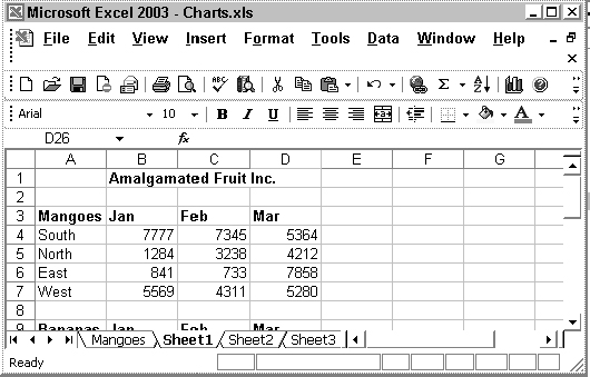
Figure 24-1

The screen in Figure 24-2 shows the chart created.

The Recorded Macro

The recorded macro should look like the following:

Sub Macro1()
'
' Macrol Macro
' Macro recorded 11/23/2003 by Paul Kimmel
'

'
    Charts.Add
    ActiveChart.ChartType = xlColumnClustered
    ActiveChart.SetSourceData Source:=Sheets(“Sheet1”).Range(“A3:D7”), PlotBy:= _
        xlRows
    ActiveChart.Location Where:=xlLocationAsNewSheet, Name:=“Mangoes”
    With ActiveChart
         .HasTitle = True
         .ChartTitle.Characters.Text = “Mangoes”
         .Axes(xlCategory, xlPrimary).HasTitle = False
         .Axes(xlValue, xlPrimary).HasTitle = False
    End With
    ActiveWindow.WindowState = xlMaximized
End Sub

The recorded macro uses the Add method of the Charts collection to create a new chart. It defines the active chart's ChartType property, and then uses the SetSourceData method to define the ranges plotted. The macro uses the Location method to define the chart as a chart sheet and assign it a name. It sets the HasTitle property to True so that it can define the ChartTitle property. Finally, it sets the HasTitle property of the axes back to False, a step which is not necessary.

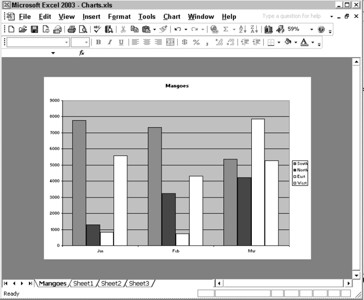
Figure 24-2

Adding a Chart Sheet Using VBA Code

The recorded code is reasonably good as it stands. However, it is more elegant to create an object variable, so that you have a simple and efficient way of referring to the chart in subsequent code. You can also remove some of the redundant code and add a chart title that is linked to the worksheet. The following code incorporates these changes:

Option Explicit

Public Sub AddChartSheet()
  Dim aChart As Chart

  Set aChart = Charts.Add
  With aChart
    .Name = “Mangoes”
    .ChartType = xlColumnClustered
    .SetSourceData Source:=Sheets(“Sheet1”).Range(“A3:D7”), PlotBy:=xlRows
    .HasTitle = True
    .ChartTitle.Text = “=Sheet1!R3C1”
  End With
End Sub

The Location method has been removed, as it is not necessary. A chart sheet is produced by default. The Chart Wizard does not allow you to enter a formula to define a title in the chart, but you can separately record changing the chart title to a formula to discover that you need to set the Text property of the ChartTitle object equal to the formula. In the preceding code, the chart title has been defined as a formula referring to the value in cell R3C1, or A3.

Embedded Charts

When you create a chart embedded as a ChartObject, it is a good idea to name the ChartObject so that it can be easily referenced in later code. You can do this by manually selecting a worksheet cell, so that the chart is not selected, then holding down Ctrl and clicking the chart. This selects the ChartObject, rather than the chart, and you will see its name to the left of the Formula bar at the top of the screen.

This is how you can tell that you have selected the ChartObject: not only does its name appear in the name box to the left of formula bar, but you will also see white boxes (white circles in Excel 2003) at each corner of the embedded chart and the middle of each edge, as shown next. If you select the chart, rather than the ChartObject, you will see black boxes.

You can select and change the name of the ChartObject in the name box and press Enter to update it. The embedded chart shown in Figure 24-3 was created using the Chart Wizard. It was then dragged to its new location and had its name changed to MangoesChart.

Using the Macro Recorder

If you select cells A3:D7 and turn on the macro recorder before creating the previous chart, including moving the ChartObject to the required location and changing its name to MangoesChart, you will get code like the following:

Sub Macro2()
'
' Macro2 Macro
' Macro recorded 11/23/2003 by Paul Kimmel
'

'

    Charts.Add
    ActiveChart.ChartType = xlColumnClustered
    ActiveChart.SetSourceData Source:=Sheets(“Sheet1”).Range(“A3:D7”), PlotBy:= _
        xlRows
    ActiveChart.Location Where:=xlLocationAsObject, Name:=“Sheet1”
    With ActiveChart
         .HasTitle = True
     .ChartTitle.Characters.Text = “Mangoes”
     .Axes(xlCategory, xlPrimary).HasTitle = False
     .Axes(xlValue, xlPrimary).HasTitle = False
   End With
   ActiveSheet.Shapes(“Chart 5”).IncrementLeft 81.75
   ActiveSheet.Shapes(“Chart 5”).IncrementTop -21.75
   ActiveWindow.Visible = False
   Windows(“Charts.xls”).Activate
   Range(“G4”).Select
   ActiveSheet.Shapes(“Chart 5”).Select
   Selection.Name = “MangoesChart”
End Sub

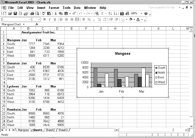
Figure 24-3

The recorded macro is similar to the one that created a chart sheet, down to the definition of the chart title, except that it uses the Location method to define the chart as an embedded chart. Up to the End With, the recorded code is reusable. However, the code to relocate the ChartObject and change its name is not reusable. The code uses the default name applied to the ChartObject to identify the ChartObject. (Note that the recorder prefers to refer to a ChartObject as a Shape object, which is an alternative that we pointed out at the beginning of this chapter.)

If you try to run this code again, or adapt it to create another chart, it will fail on the reference to Chart 30, or whichever shape you created when you recorded the macro. It is not as obvious how to refer to the ChartObject itself as how to refer to the active chart sheet.

Adding an Embedded Chart Using VBA Code

The following code uses the Parent property of the embedded chart to identify the ChartObject containing the chart:

Sub AddChart()
  Dim aChart As Chart

  ActiveSheet.ChartObjects.Delete
  Set aChart = Charts.Add
  Set aChart = aChart.Location(Where:=xlLocationAsObject, Name:=“Sheet1”)
  With aChart
    .ChartType = xlColumnClustered
    .SetSourceData Source:=Sheets(“Sheet1”).Range(“A3:D7”), _
      PlotBy:=xlRows
    .HasTitle = True
    .ChartTitle.Text = “=Sheet1!R3C1”
    With .Parent
       .Top = Range(“F3”).Top
       .Left = Range(“F3”).Left
       .Name = “MangoesChart”
    End With
  End With
End Sub

AddChart first deletes any existing ChartObjects. It then sets the object variable aChart to refer to the added chart. By default, the new chart is on a chart sheet, so the Location method is used to define the chart as an embedded chart.

AddChart defines the chart type, source data, and chart title. Again, the chart title has been assigned a formula referring to cell A3. Using the Parent property of the Chart object to refer to the ChartObject object, AddChart sets the Top and Left properties of the ChartObject to be the same as the Top and Left properties of cell F3. AddChart finally assigns the new name to the ChartObject so that it can easily be referenced in the future.

Editing Data Series

The SetSourceData method of the Chart object is the quickest way to define a completely new set of data for a chart. You can also manipulate individual series using the Series object, which is a member of the chart's SeriesCollection object. The following example is designed to show you how to access individual series.

We will take the MangoesChart and delete all the series from it, and then replace them with four new series, one at a time. The new chart will contain product information for a region nominated by the user. To make it easier to locate each set of product data, names have been assigned to each product range in the worksheet. For example, A3:D7 has been given the name Mangoes, corresponding to the label in A3. The final chart will be similar to Figure 24-4.

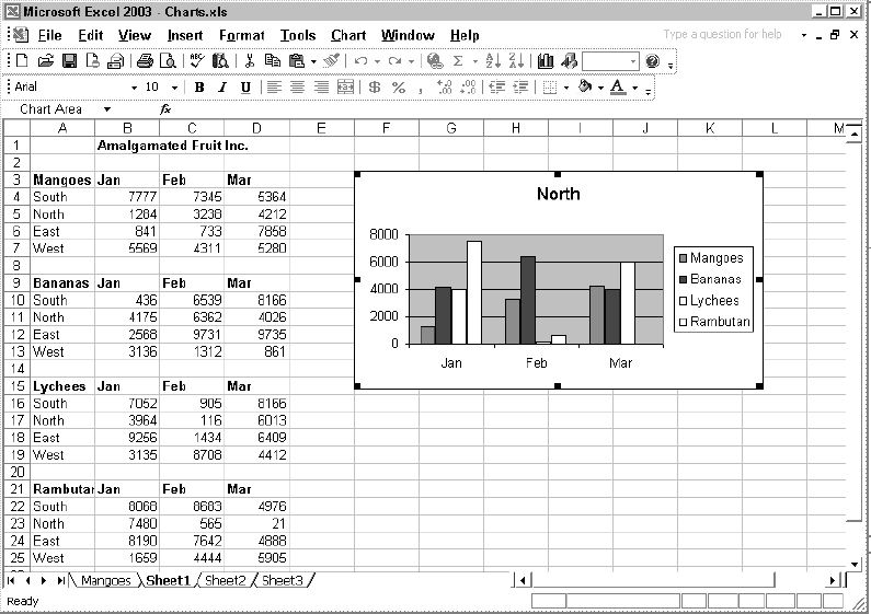
Figure 24-4

The following code converts MangoesChart to include the new data (note that the original chart must still be on the spreadsheet for this to work). As MangoesToRegion comprises several parts, we'll examine it by section. (The complete for MangoesToRegion listing is provided here and the supporting methods are described later.)

Public Function PickRegion() As Integer

  Dim Answer As String
  Do
    Answer = InputBox(“Enter Region number (1 to 4)”)
    If Answer >= “1” And Answer <= “4” Then
      Exit Do
    Else
      Call MsgBox(“Region must be be 1, 2, 3 or 4”, vbCritical)
    End If
  Loop

  PickRegion = CInt(Answer)
End Function

Public Sub MangoesToRegion()

  Debug.Assert MangoChartExists()

  ' Sentinel: No point in doing anything if pre-conditions don't exist
  If Not MangoChartExists() Then
    MsgBox “MangoesChart was not found - procedure aborted”, vbCritical
    Exit Sub
  End If

  Dim aChart As Chart
  Set aChart = GetMangoChart().Chart
  Debug.Assert (aChart Is Nothing = False)

  Call DeleteSeries(aChart.SeriesCollection)
  Call AddProductsForRegion(PickRegion(), aChart)
End Sub

PickRegion shows the user an InputBox with text indicating that valid choices are 1, 2, 3, and 4. MangoesToRegion asserts that the original Mangoes chart exists. The Debug.Assert is for our use as developers. Next, the sentinel checks to ensure that the chart exists; this second check is for consumers. Next, we get the Chart object—from GetMangoChart, which returns the ChartObject—from the ChartObject returned by GetMangoChart. And, we finish up by deleting the existing chart series and adding a new series for the selected information (Mangoes, Bananas, Lychees, or Rambutan):

Public Sub MangoesToRegion()

  Debug.Assert MangoChartExists()

  ' Sentinel: No point in doing anything if pre-conditions don't exist
  If Not MangoChartExists() Then
    MsgBox “MangoesChart was not found - procedure aborted”, vbCritical
    Exit Sub
  End If

  Dim aChart As Chart
  Set aChart = GetMangoChart().Chart
  Debug.Assert (aChart Is Nothing = False)

  Call DeleteSeries(aChart.SeriesCollection)
  Call AddProductsForRegion(PickRegion(), aChart)
End Sub

This very concise code is supported by the cast of methods MangoChartExists, GetMangoChart, DeleteSeries, AddProductsForRegion, and PickRegion. Let's review each of those methods in the order introduced:

Public Function MangoChartExists() As Boolean
  MangoChartExists = GetMangoChart Is Nothing = False
End Function

MangoChartExists call GetMangoChart and tests to ensure that a valid ChartObject is returned. GetMangoChart uses an error handler to attempt to get the chart returning Nothing if an error occurs or the chart is not found:

Public Function GetMangoChart() As ChartObject
  On Error GoTo Catch
    Set GetMangoChart = Worksheets(“Sheet1”).ChartObjects(“MangoesChart”)
  Exit Function

Catch:
  Set GetMangoChart = Nothing
End Function

Next, DeleteSeries accepts a SeriesCollection, which we obtain from the Chart object, and it walks through preexisting series deleting each:

Public Sub DeleteSeries(ByVal Series As SeriesCollection)

  Dim I As Integer
  For I = Series.Count To 1 Step -1
    Series(I).Delete
  Next I
End Sub

After we delete the existing series, we can create a new series and add all of the products from the selected named group of information and finish up by adding a title and name to the new series:

Public Sub AddProductsForRegion(ByVal region As Integer, _
  ByVal Chart As Chart)

  Dim I As Integer
  Dim J As Integer
  Dim rangeY As Range
  Dim rangeX As Range
  Dim products As Variant
  Dim regions As Variant

  products = Array(“Mangoes”, “Bananas”, “Lychees”, “Rambutan”)
  regions = Array(“South”, “North”, “East”, “West”)

  For I = LBound(products) To UBound(products)
    Set rangeY = Range(products(I)).Offset(region, 1).Resize(1, 3)
    Set rangeX = Range(products(I)).Offset(0, 1).Resize(1, 3)
    With Chart.SeriesCollection.NewSeries
      .Name = products(I)
      .Values = rangeY
      .XValues = “=” & rangeX.Address _
          (RowAbsolute:=True, _
      ColumnAbsolute:=True, _
      ReferenceStyle:=xlR1C1, _
      External:=True)
    End With
  Next I

  Chart.ChartTitle.Text = regions(region - 1 + LBound(regions))
  GetMangoChart().Name = “RegionChart”
End Sub

That's all there is to it. In a nutshell, we picked an existing chart, deleted the existing series data, and added the new data. We prefer to break up methods as demonstrated in the preceding example because it permits us to legitimately reduce unnecessary comments and eliminate extra local, temporary variables.

If you have been programming for the last 10 years or more then you may be comfortable with a lot of temporary variables and long, monolithic methods. That style of programming isn't wrong, but modern discoveries in software development, including Refactoring—which applies as much to VBA as any other object-oriented language—argue successfully that code is more manageable with shorter methods, fewer temporaries, and well-named methods instead of a lot of temporary variables. We encourage you to read Martin Fowler's Refactoring: Improving the Design of Existing Code (Addison-Wesley, 1999) for more information.

Defining Chart Series with Arrays

A chart series can be defined by assigning a VBA array to its Values property. This can come in handy if you want to generate a chart that is not linked to the original data. The chart can be distributed in a separate workbook that is independent of the source data.

Figure 24-5 shows a chart of the Mangoes data. You can see the definition of the first data series in the Formula bar above the worksheet. The month names and the values on the vertical axis are defined by Excel arrays. The region names have been assigned as text to the series names.

The 3D chart can be created using the following code:

Public Sub MakeArrayChart()
  Dim sourceWorksheet As Worksheet
  Dim sourceRange As Range
  Dim aWorkbook As Workbook
  Dim aWorksheet As Worksheet
  Dim aChart As Chart
  Dim aNewSeries As Series
  Dim I As Integer
  Dim SalesArray As Variant
  Dim MonthArray As Variant

  MonthArray = Array(“Jan”, “Feb”, “Mar”)

  'Define the data source
  Set sourceWorksheet = ThisWorkbook.Worksheets(“Sheet1”)
  Set sourceRange = sourceWorksheet.Range(“Mangoes”)

  'Create a new workbook
  Set aWorkbook = Workbooks.Add
  Set aWorksheet = aWorkbook.Worksheets(1)

  'Add a new chart object and embed it in the worksheet
  Set aChart = aWorkbook.Charts.Add
  Set aChart = aChart.Location(Where:=xlLocationAsObject, Name:=“Sheet1”)

  With aChart
    'Define the chart type
    .ChartType = xl3DColumn
    For I = 1 To 4
      'Create a new series
      Set aNewSeries = .SeriesCollection.NewSeries
      'Assign the data as arrays
      SalesArray = sourceRange.Offset(I, 1).Resize(1, 3).Value
      aNewSeries.Values = SalesArray
      aNewSeries.XValues = MonthArray
      aNewSeries.Name = sourceRange.Cells(I + 1, 1).Value
    Next I

    .HasLegend = False
    .HasTitle = True
    .ChartTitle.Text = “Mangoes”
    'Position the ChartObject in B2:I22 and name it
    With .Parent
      .Top = aWorksheet.Range(“B2”).Top
      .Left = aWorksheet.Range(“B2”).Left
      .Width = aWorksheet.Range(“B2:I22”).Width
      .Height = aWorksheet.Range(“B2:I22”).Height
      .Name = “ArrayChart”
    End With
  End With
End Sub

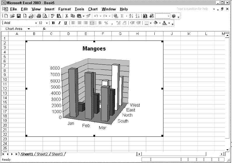
Figure 24-5

(The named range Mangoes was added using the Insert Name Define Excel menu item and specifying the cells A3 to D7 as the Mangoes range.) MakeArrayChart assigns the month names to MonthArray. This data could have come from the worksheet, if required, like the sales data. A reference to the worksheet that is the source of the data is assigned to sourceWorksheet. The Mangoes range is assigned to sourceRange. A new workbook is created for the chart and a reference to it is assigned to aWorkbook. A reference to the first worksheet in the new workbook is assigned to aWorksheet. A new chart is added to the Charts collection in aWorkbook and a reference to it assigned to aChart. The Location method converts the chart to an embedded chart and redefines aChart.

In the With…End With structure, the ChartType property of aChart is changed to a 3D column type. The For…Next loop creates the four new series. Each time around the loop, a new series is created with the NewSeries method. The region data from the appropriate row is directly assigned to the variant SalesArray, and SalesArray is immediately assigned to Values property of the new series.

MonthArray is assigned to the XValues property of the new series. The text in column A of the Mangoes range is assigned to the Name property of the new series.

The code then removes the chart legend, which is added by default, and sets the chart title. The final code operates on the ChartObject, which is the chart's parent, to place the chart exactly over B2:I22, and name the chart ArrayChart.

The result is a chart in a new workbook that is quite independent of the original workbook and its data. If the chart had been copied and pasted into the new workbook, it would still be linked to the original data.

Converting a Chart to use Arrays

You can easily convert an existing chart to use arrays instead of cell references and make it independent of the original data is was based on. The following code shows how:

Public Sub ConvertSeriesValuesToArrays()
  Dim aSeries As Series
  Dim aChart As Chart

  On Error GoTo Catch

  Set aChart = ActiveSheet.ChartObjects(1).Chart
  For Each aSeries In aChart.SeriesCollection
    aSeries.Values = aSeries.Values
    aSeries.XValues = aSeries.XValues
    aSeries.Name = aSeries.Name
  Next aSeries

  Exit Sub
Catch:

  MsgBox “Sorry, the data exceeds the array limits”
End Sub

For each series in the chart, the Values, XValues, and Name properties are set equal to themselves. Although these properties can be assigned range references, they always return an array of values when they are interrogated. This behavior can be exploited to convert the cell references to arrays.

Bear in mind that the number of data points that can be contained in an array reference is limited to 250 characters, or thereabouts. The code will fail if the limits are exceeded, so we have set up an error trap to cover this possibility.

Determining the Ranges used in a Chart

The behavior that is beneficial when converting a chart to use arrays is a problem when you need to programmatically determine the ranges that a chart is based on. If the Values and Xvalues properties returned the strings that you use to define them, the task would be easy.

The only property that contains information on the ranges is the Formula property that returns the formula containing the SERIES function as a string. The formula would be like the following:

=SERIES(Sheet1!$A$4, Sheet1!$B$3:$D$3, Sheet1!$B$4:$D$4,1)

The XValues are defined by the second parameter and the Values by the third parameter. You need to locate the commas and extract the text between them as shown in the following code, designed to work with a chart embedded in the active sheet:

Public Sub GetRangesFromChart()
  Dim aSeries As Series
  Dim seriesFunction As String
  Dim firstComma As Integer
  Dim secondComma As Integer
  Dim thirdComma As Integer
  Dim rangeValueString As String
  Dim rangeXValueString As String
  Dim rangeValue As Range
  Dim rangeXValue As Range

  On Error GoTo Catch

  'Get the SERIES function from the first series in the chart
  Set aSeries = ActiveSheet.ChartObjects(1).Chart.SeriesCollection(1)
  seriesFunction = aSeries.Formula

  'Locate the commas
  firstComma = InStr(1, seriesFunction, “,”)
  secondComma = InStr(firstComma + 1, seriesFunction, “,”)
  thirdComma = InStr(secondComma + 1, seriesFunction, “,”)
  'Extract the range references as strings
  rangeXValueString = Mid(seriesFunction, firstComma + 1, _
    secondComma - firstComma - 1)

  rangeValueString = Mid(seriesFunction, secondComma + 1, _
    thirdComma - secondComma - 1)

  'Convert the strings to range objects
  Set rangeXValue = Range(rangeXValueString)
  Set rangeValue = Range(rangeValueString)
  'Colour the ranges
  rangeXValue.Interior.ColorIndex = 3
  rangeValue.Interior.ColorIndex = 4
  Exit Sub

Catch:
  MsgBox “Sorry, an error has ocurred” & vbCr & _
         “This chart might contain invalid range references”
End Sub

seriesFunction is assigned the formula of the series, which contains the SERIES function as a string. The positions of the first, second, and third commas are found using the InStr function. The Mid function is used to extract the range references as strings and they are converted to Range objects using the Range property.

The conversion of the strings to Range objects works even when the range references are not on the same sheet or in the same workbook as the embedded chart, as long as the source data is in an open workbook.

You could then proceed to manipulate the Range objects. You can change cell values in the ranges, for example, or extend or contract the ranges, once you have programmatic control over them. We have just colored the ranges for illustration purposes.

Chart Labels

In Excel, it is easy to add data labels to a chart, as long as the labels are based on the data series values or X-axis values. These options are available using Chart Chart Options.

You can also enter your own text as labels, or you can enter formulas into each label to refer to cells, but this involves a lot of manual work. You would need to add standard labels to the series and then individually select each one and either replace it with your own text, or click in the Formula bar and enter a formula. Alternatively, you can write a macro to do it for you.

Figure 24-6 shows a chart of sales figures for each month, with the name of the top salesperson for each month. The labels have been defined by formulas linked to row 4 of the worksheet, as you can see for Jenny in April. The formula in the Formula bar points to cell E4.

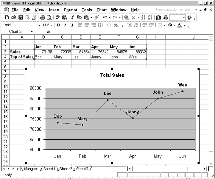
Figure 24-6

Say, you have set up a line chart like the previous one, but without the data labels. You can add the data labels and their formulas using the following code:

Public Sub AddDataLabels()
    Dim sales As Series
    Dim points As points
    Dim aPoint As Point
    Dim aRange As Range
    Dim I As Integer

    Set aRange = Range(“B4:G4”)
    Set sales = ActiveSheet.ChartObjects(1).Chart.SeriesCollection(1)
    sales.HasDataLabels = True
    Set points = sales.points
    For Each aPoint In points
      I = I + 1
      aPoint.DataLabel.Text = “=” & aRange.Cells(I).Address _
        (RowAbsolute:=True, _
        ColumnAbsolute:=True, _
        ReferenceStyle:=xlR1C1, _
        External:=True)
        aPoint.DataLabel.Font.Bold = True
        aPoint.DataLabel.Position = xlLabelPositionAbove
  Next aPoint
End Sub

The object variable aRange is assigned a reference to B4:G4. The sales variable is assigned a reference to the first, and only, series in the embedded chart and the HasDataLabels property of the series is set to True. The For Each…Next loop processes each point in the data series. For each point, the code assigns a formula to the Text property of the point's data label. The formula refers to the worksheet cell as an external reference in R1C1 format. The data label is also made bold and the label positioned above the data point.

Summary

It is easy to create a programmatic reference to a chart on a chart sheet. The Chart object is a member of the Charts collection of the workbook. To reference a chart embedded in a worksheet, you need to be aware that the Chart object is contained in a ChartObject object that belongs to the ChartObjects collection of the worksheet.

You can move or resize an embedded chart by changing the Top, Left, Width, and Height properties of the ChartObject. If you already have a reference to the Chart object, you can get a reference to the ChartObject object through the Parent property of the Chart object.

Individual series in a chart are Series objects, and belong to the SeriesCollection object of the chart. The Delete method of the Series object is used to delete a series from a chart. You use the NewSeries method of the SeriesCollection object to add a new series to a chart.

You can assign a VBA array, rather than the more commonly used Range object, to the Values property of a Series object. This creates a chart that is independent of worksheet data and can be distributed without a supporting worksheet.

The Values and XValues properties return data values, not the range references used in a chart. You can determine the ranges referenced by a chart by examining the SERIES function in the Formula property of each series.

The data points in a chart are Point objects and belong to the Points collection of the Series object. Excel does not provide an easy way to link cell values to labels on series data points through the user interface. However, links can be easily established to data point labels using VBA code.