
Chapter 7
Sorting and Filtering Data
Perform a Simple Sort or Filter
You can make a range easier to analyze by sorting it based on a column’s values. You can sort the data using either an ascending sort, which arranges the values alphabetically from A to Z or numerically from 0 to 9, or a descending sort, which arranges the values from Z to A or from 9 to 0.
You can also analyze data by filtering it to show only the items you want to work with. The easiest way to filter a range is to use the Filter buttons, each of which presents you with a list of check boxes for each unique value in a column. You filter the data by activating the check boxes for the items you want to see.
Perform a Simple Sort or Filter
Sort a List

![]() Click a cell in the column you want to sort.
Click a cell in the column you want to sort.
![]() Click the Data tab.
Click the Data tab.
![]() Click a sort direction.
Click a sort direction.
A Click Sort A to Z to sort from lowest to highest — ascending order.
B Click Sort Z to A to sort from highest to lowest — descending order.

C Excel sorts your list by the column you selected.
Filter a List

![]() Click a cell in the range you want to filter.
Click a cell in the range you want to filter.
![]() Click the Data tab.
Click the Data tab.
![]() Click Filter.
Click Filter.
D AutoFilter buttons appear next to your field headers.
![]() Click an AutoFilter button.
Click an AutoFilter button.
The Sort & Filter menu appears.
![]() Click items to deselect the ones you do not want (
Click items to deselect the ones you do not want (![]() changes to
changes to ![]() ).
).
![]() Click OK.
Click OK.
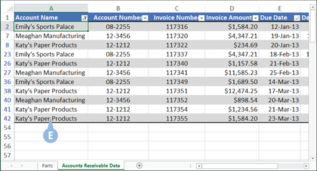
E Excel filters your list.
EXTRA
When you activate the Data tab’s Filter button (![]() ), Excel places an AutoFilter button (
), Excel places an AutoFilter button (![]() ) next to each column header. When you filter the data using a particular field, Excel modifies that field’s AutoFilter button to include a Field Filter icon (
) next to each column header. When you filter the data using a particular field, Excel modifies that field’s AutoFilter button to include a Field Filter icon (![]() ). Similarly, when you sort a column in ascending order, Excel modifies that field’s AutoFilter to include a Field Sort Ascending button (
). Similarly, when you sort a column in ascending order, Excel modifies that field’s AutoFilter to include a Field Sort Ascending button (![]() ). When you sort a column in descending order, Excel modifies that field’s AutoFilter to include a Field Sort Descending button (
). When you sort a column in descending order, Excel modifies that field’s AutoFilter to include a Field Sort Descending button (![]() ). To clear all filters, click the Data tab and then click Clear Filter (
). To clear all filters, click the Data tab and then click Clear Filter (![]() ). To remove the AutoFilter buttons next to your field names, click the Data tab and then click Filter (
). To remove the AutoFilter buttons next to your field names, click the Data tab and then click Filter (![]() ).
).
Perform a Multilevel Sort
A simple sort is one that arranges data based on the contents of a single column. Simple sorts are fine for many data analysis applications, but Excel enables you to take sorting to a higher level. Specifically, you can sort your data on two or more fields, creating a multilevel sort.
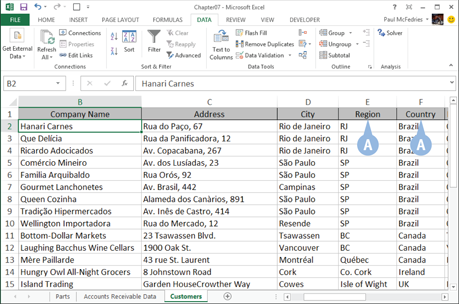
For example, with a database of customer information, a simple sort might organize that data in ascending order by country name. However, within each country, you might also want the customers sorted by region (such as the state or province). You do that by creating a multilevel sort where the country is the first level and the region is the second level.
Perform a Multilevel Sort

![]() Click a cell in the range you want to sort.
Click a cell in the range you want to sort.
![]() Click the Data tab.
Click the Data tab.
![]() Click Sort.
Click Sort.
The Sort dialog box appears.
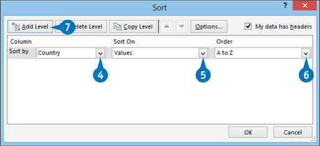
![]() Under Column, click the Sort by down arrow and then click the column you want to use as the first sort level.
Under Column, click the Sort by down arrow and then click the column you want to use as the first sort level.
![]() Under Sort On, click the Sort by down arrow and then click Values.
Under Sort On, click the Sort by down arrow and then click Values.
![]() Under Order, click the Sort by down-arrow and then click a sort order.
Under Order, click the Sort by down-arrow and then click a sort order.
![]() Click Add Level.
Click Add Level.

![]() Under Column, click the Then by down arrow and then click the column you want to use for this sort level.
Under Column, click the Then by down arrow and then click the column you want to use for this sort level.
![]() Under Sort On, click the Then by down arrow and then click Values.
Under Sort On, click the Then by down arrow and then click Values.
![]() Under Order, click the Then by down arrow and then click a sort order.
Under Order, click the Then by down arrow and then click a sort order.
![]() Repeat steps 7 to 10 to add additional sort levels.
Repeat steps 7 to 10 to add additional sort levels.
![]() Click OK.
Click OK.
A Excel sorts the list.
EXTRA
If you are sorting a table, click any cell in the table and Excel selects the entire table when you open the Sort dialog box. If you are sorting a range of cells that are not a table, select the cells and then open the Sort dialog box. If your data does not have column headers, deselect the My Data Has Headers check box (![]() changes to
changes to ![]() ).
).
To rearrange the sort levels, follow steps 1 to 3 to open the Sort dialog box, click a level, and then click either Move Up (![]() ) or Move Down (
) or Move Down (![]() ). To remove a sort level, open the Sort dialog box, click the level you want to remove, and then click Delete Level.
). To remove a sort level, open the Sort dialog box, click the level you want to remove, and then click Delete Level.
Create a Custom Sort
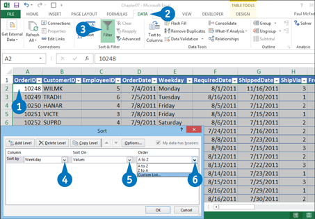
When you are analyzing data, you might find that a standard ascending or descending sort is what you need. For example, you might prefer to sort your dates by the weekday name or month name. You can perform such sorts by basing them on a custom list of values.
Excel comes with several predefined custom lists that enable you to sort dates by weekday names or month names. However, if your range data includes a unique set of values, or if you have a data series that you use often, you can create a custom list based on the values, and then use that list for sorting the range.
Create a Custom Sort
![]() Click a cell in the range you want to sort.
Click a cell in the range you want to sort.
![]() Click the Data tab.
Click the Data tab.
![]() Click the Sort button.
Click the Sort button.
The Sort dialog box appears.
![]() Click here and then click the column you want to use as the first sort level.
Click here and then click the column you want to use as the first sort level.
![]() Click here and then click Values.
Click here and then click Values.
![]() Click here and then click Custom List.
Click here and then click Custom List.
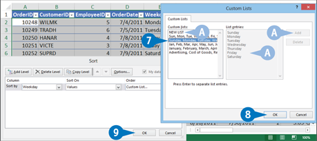
The Custom Lists dialog box appears.
![]() Click the list you want to use as the sort order.
Click the list you want to use as the sort order.
A To create your own custom list, click NEW LIST, type your entries, and then click Add.
![]() Click OK.
Click OK.
![]() Click OK.
Click OK.
Excel sorts the data using the custom list.
Sort by Cell Color, Font Color, or Cell Icon
You can use conditional formatting to format your data with cell colors, font colors, or cell icons. You can then use the Sort dialog box to sort data based on one or more of these formats. When you choose Cell Color, Font Color, or Cell Icon in the Sort On drop-down list of the Sort dialog box, Excel places a list of cell colors, font colors, or cell icons in the Order field. You can then choose On Top to place the selection on the next highest level or On Bottom to place the selection on the next lowest level.
Sort by Cell Color, Font Color, or Cell Icon
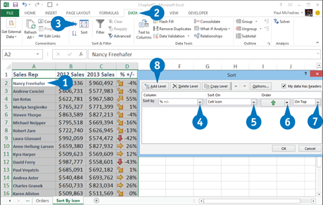
![]() Click a cell in the range you want to sort.
Click a cell in the range you want to sort.
![]() Click the Data tab.
Click the Data tab.
![]() Click Sort.
Click Sort.
The Sort dialog box appears.
![]() Click here and then select a sort column.
Click here and then select a sort column.
![]() Click here and then select Cell Color, Font Color, or Cell Icon.
Click here and then select Cell Color, Font Color, or Cell Icon.
![]() Click here and then select a cell color, font color, or cell icon.
Click here and then select a cell color, font color, or cell icon.
![]() Click here and then select On Top or On Bottom.
Click here and then select On Top or On Bottom.
![]() Click Add Level.
Click Add Level.
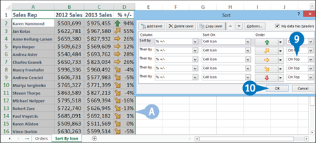
![]() Repeat steps 4 to 8 until you are finished.
Repeat steps 4 to 8 until you are finished.
![]() Click OK.
Click OK.
A Excel sorts the column by cell color, font color, or cell Icon.
Using Quick Filters for Complex Sorting
When you filter a range using a filter list, you filter the data by selecting the check boxes for the records you want to see. A more complex technique uses quick filters, which enable you to specify criteria for a field, such as only showing those records where the field value is greater than a specified amount.
Excel offers three types of quick filters: date filters for date fields; text filters for text fields; and number filters for numeric fields. When you select one of these options, a menu appears. From this menu, you can select the criteria you want to apply. You can also apply multiple filters.
Using Quick Filters for Complex Sorting

![]() Click a cell in the range you want to filter.
Click a cell in the range you want to filter.
![]() Click the Data tab.
Click the Data tab.
![]() Click Filter.
Click Filter.
A AutoFilter buttons appear next to your field headers.
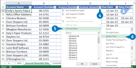
![]() Click an AutoFilter button.
Click an AutoFilter button.
![]() Click Number Filters.
Click Number Filters.
Note: If the field is a date field, click Date Filters; if the field is a text field, click Text Filters.
![]() Click the filter you want to use.
Click the filter you want to use.
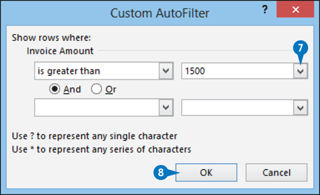
The Custom AutoFilter dialog box appears.
Note: Some quick filters do not require extra input, so you can skip the next two steps.
![]() Type the value you want to use, or click the down arrow and select a unique value from the drop-down list.
Type the value you want to use, or click the down arrow and select a unique value from the drop-down list.
![]() Click OK.
Click OK.
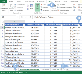
B Excel filters the table to show only those records that have the field values you selected.
C Excel displays the number of records found.
D If you have AutoFilter buttons displayed, the field’s button displays a filter icon.
E To remove the filter, click Clear.
APPLY IT
You can create custom quick filters that use two different criteria, and you can tell Excel to filter records that match both or at least one of the two criteria. Follow steps 1 to 5 and then click Custom Filter. The Custom AutoFilter dialog box offers two sets of list boxes. Use the lists on the left to choose operators, such as Equal and Is Greater Than; use the lists on the right to specify field values.
If you want Excel to match both criteria, click the And option (![]() changes to
changes to ![]() ); if you want Excel to match at least one of the criteria, click the Or option (
); if you want Excel to match at least one of the criteria, click the Or option (![]() changes to
changes to ![]() ). Click OK.
). Click OK.
Enter Criteria to Find Records
Once you have converted a range to a table, you may want to retrieve specific information. Using the Excel Advanced Filter, you can set up complex filters and use them to limit the data you retrieve.
When using the Advanced Filter feature, you must set up a worksheet area called the criteria range. In the criteria range, you tell Excel exactly what you are looking for. For example, you can tell Excel you want to retrieve all people with an income of $100,000 or more.
Types of Criteria
You can use two types of criteria to find records: comparison criteria and computed criteria. With comparison criteria, you enter your criteria underneath a field label. For example, if you want to find all people with an income greater than $100,000, you enter >100000 under the criteria range field labeled Income, as shown here.
Criteria Range
![]()
Table

With computed criteria, you use a formula to find records. You use computed criteria when your table does not have a field that specifies the data you want to use as the filter. For example, if you want to extract all records from the table where the property tax plus the income tax is greater than $20,000, you can use the formula =Property Tax+Income Tax>20000 as your criteria.
When you use computed criteria, at least one variable in the formula must be a field in your table. However, the criteria range label cannot be one of the field labels used by your table. For example, you can create a new criteria range label called Total Tax and place your formula under that label. Excel interprets all criteria that use field labels from your table as comparison criteria. Excel interprets all criteria that do not use field labels as computed criteria. The following is an example of computed criteria.
Criteria Range
![]()
Set Up Your Criteria Range
You can place your criteria range anywhere in your workbook, but the best places are above your table or on a separate worksheet. You should create one row that lists your field labels. You do not have to include all your labels, but you must include every label for which you are going to enter comparison criteria. You should also place the labels that you are going to use for computed criteria on this row. You also need at least one additional row to use for the criteria.
Enter Comparison Criteria
You can use comparison criteria to find text, numbers, dates, and logical values. If you want to match a series of characters, you can place the characters under the field label. For example, if you want to find all records for people with the last name Jones, you type Jones under the field label Last Name in the criteria range.
For more flexibility with text criteria, you can use wildcard characters. You use a question mark (?) to match any single character. For example, J?ne finds Jane and June. You use an asterisk (*) to match any series of characters. For example, *son finds Jackson and Johnson. If you need to find a question mark or an asterisk, you can place a tilde (~) in front of the question mark or asterisk. Excel assumes that there is an asterisk after every search entry. Therefore, if you type John under the Last Name field label, Excel finds everyone whose last name begins with John. If you want to find an exact match for a text value, you can enter your criteria in the format =”=text”. For example, if you want to find John, but not Johnson, you type =”=John”.
You can also use comparison operators. To do this, you type the comparison operator followed by the value you are trying to find. For example, to find all records where the income is equal to or greater than $100,000, you type >=100000 under the Income field label. To find all last names that are alphabetically greater than Cohen, you type >Cohen under the Last Name field label. Comparison criteria are not case-sensitive. To find all blank fields, you type an equal sign with nothing after it. To find all nonblank fields, you type the unequal operator (<>) with nothing after it. To learn more about comparison operators, see Chapter 1.
Enter Computed Criteria
When you enter computed criteria, you must use a formula that evaluates to the logical value TRUE or the logical value FALSE, based on whether your criteria match records in your table, and your formula must include a reference to at least one field label from your table. If you use computed criteria, your field labels must conform to the rules for naming a range. To learn more about naming ranges, see Chapter 1.
You create your formula by using a relative cell reference to the first data row in your table. For example, =C8+D8>20000 is a valid formula if the first data row in your formula is row 8. If you name the data fields in the first row of your table, you can use range names in your formula. For example, if C8 is named Property Tax and D8 is named Income Tax, you can use the formula =Property Tax + Income Tax > 20000.
You create a new label and place your formula under that label in the criteria range. The cell displays either the value TRUE or the value FALSE.
Apply Multiple Criteria
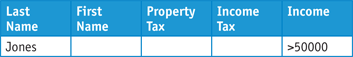
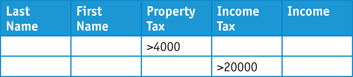
You can use a criteria range to specify multiple criteria. For example, you can find all people with the last name Jones whose incomes are more than $50,000. You can also find all people whose property tax is more than $4,000 or whose income tax is more than $20,000. To meet both criteria, you can place your criteria on the same row. To meet either criterion, you can place your criteria on separate rows.
Meet both criteria:
Meet either criterion:
Create an Advanced Filter
You can go beyond the limitations of the AutoFilter command by creating an advanced filter that uses criteria to specify the records you want to see. You have two options when creating an advanced filter: you can have the filtered items appear in place, under the column headings of your table; or, you can have your filtered items appear in another location, thereby, enabling you to also view your original table data. If you choose the latter, you should select a worksheet location beside or below the original table and make sure the location has enough room below it to include all the values that Excel returns in the filter results. For more information on using criteria, see the section, Enter Criteria to Find Records.
Create an Advanced Filter
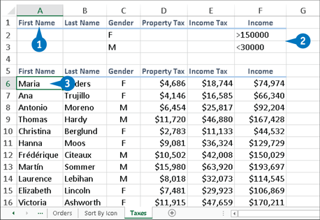
![]() Set up your criteria range by typing the headings for the columns you want to filter.
Set up your criteria range by typing the headings for the columns you want to filter.
Note: In most cases, it is easiest just to copy the column headings from the original table.
![]() Type the criteria you want to use for your filter.
Type the criteria you want to use for your filter.
![]() Click a cell inside the original table.
Click a cell inside the original table.
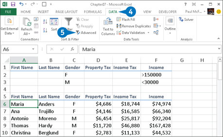
![]() Click the Data tab.
Click the Data tab.
![]() Click Advanced.
Click Advanced.
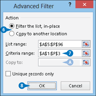
The Advanced Filter dialog box appears.
![]() Select where to place the filter results (
Select where to place the filter results (![]() changes to
changes to ![]() ).
).
![]() Enter the criteria range address, including the column headings.
Enter the criteria range address, including the column headings.
A If you chose Copy to Another Location in step 6, enter the first cell of the copy location.
![]() Click OK.
Click OK.
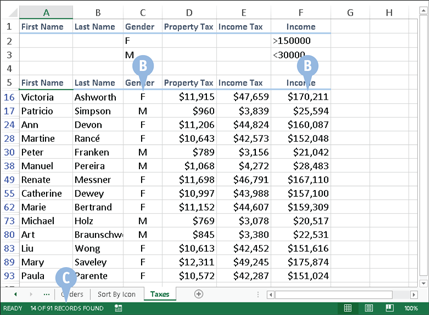
B Excel filters the table to show only those records that have the field values you selected.
C Excel displays the number of records found.
Display Unique Records in the Filter Results
It is not uncommon to have a range or table with duplicate items, meaning the values in two or more rows are identical. For example, a simple list of books sold over some time will likely have duplicate entries. As part of your data analysis, you might prefer to see only the unique values in the range.
You can use the advanced filtering tool in Excel to identify and filter the duplicates. You must specify a criteria range by which you want to filter your data. Your criteria consist of at least two rows, one with one or more headings and the other with the criteria. See the section, Enter Criteria to Find Records, for information on how to set up your criteria range.
Display Unique Records in the Filter Results
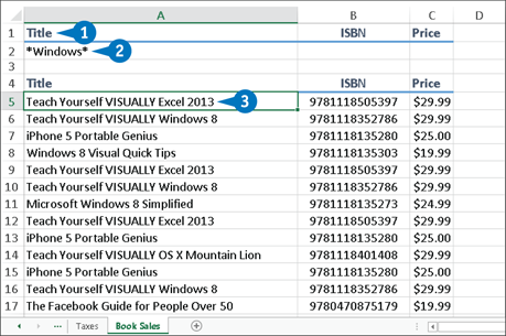
![]() Set up your criteria range by typing the headings for the columns you want to filter.
Set up your criteria range by typing the headings for the columns you want to filter.
Note: In most cases, it is easiest just to copy the column headings from the original table.
![]() Type the criteria you want to use for your filter.
Type the criteria you want to use for your filter.
![]() Click a cell inside the original table.
Click a cell inside the original table.
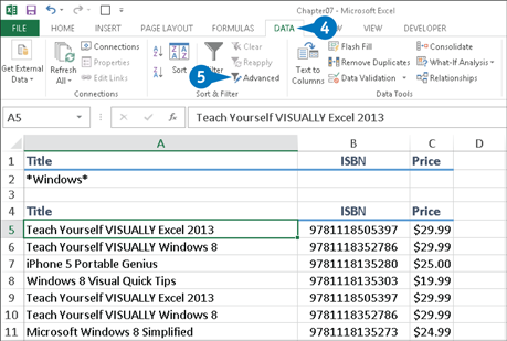
![]() Click the Data tab.
Click the Data tab.
![]() Click Advanced.
Click Advanced.
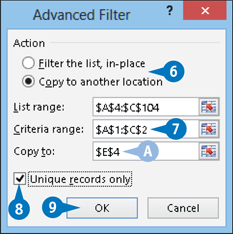
The Advanced Filter dialog box appears.
![]() Select where to place the filter results (
Select where to place the filter results (![]() changes to
changes to ![]() ).
).
![]() Enter the criteria range address, including the column headings.
Enter the criteria range address, including the column headings.
A If you chose Copy to Another Location in step 6, enter the first cell of the copy location.
![]() Click the Unique Records Only check box (
Click the Unique Records Only check box (![]() changes to
changes to ![]() ).
).
![]() Click OK.
Click OK.

B In this example, Excel copies the unique records from the filter results to the specified location.
Count Filtered Records
When you filter a range or table using an AutoFilter, a quick filter, or an advanced in-place filter, Excel uses the status bar to display the number of records returned in the filter results. That is useful information, but in your analysis of the data, you might need to use that count value in a formula.
You can do this by using DCOUNT, one of the database functions in Excel, which returns the number of items in a range that satisfy your criteria. DCOUNT takes three arguments: database specifies the range that contains the data; field specifies the column you want to count; and criteria specifies the address of the criteria range.
Count Filtered Records

![]() Set up your criteria range by typing the headings for the columns you want to filter.
Set up your criteria range by typing the headings for the columns you want to filter.
Note: In most cases, it is easiest just to copy the column headings from the original table.
![]() Type the criteria you want to use for your filter.
Type the criteria you want to use for your filter.
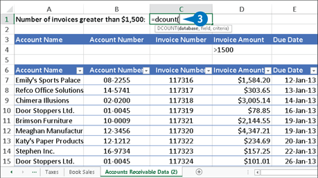
![]() In the cell where you want the count result to appear, type =dcount(.
In the cell where you want the count result to appear, type =dcount(.
Note: The DCOUNT function counts only cells containing numbers. For non-numeric data, use the DCOUNTA function.

![]() Enter the address or name of the data range.
Enter the address or name of the data range.
Note: As shown here, if the data is in a table, type the table name followed by [#All].
![]() Type the column name in quotation marks.
Type the column name in quotation marks.
Alternatively, type the column number.
![]() Type the address of the criteria range.
Type the address of the criteria range.
![]() Type 20.
Type 20.
![]() Click the Enter button or press Enter.
Click the Enter button or press Enter.

A Excel displays the count of the records that match the criteria.