Chapter 4
Analyzing Financial Data
Calculate Future Value
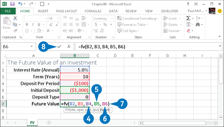
If you have $1,000 and you plan to invest it at 5 percent interest, compounded annually for ten years, the amount you will receive at the end of ten years is called the future value of $1,000. You can use the Excel FV function to calculate the amount you will receive.
FV takes five arguments: rate, the interest rate; nper, the term of the investment; pmt, the amount of each deposit into the investment; the optional pv, your initial investment; and the optional type, a number indicating when deposits are due (0 or blank for end-of-period; 1 for beginning-of-period). When you are working with FV, cash outflows are considered negative amounts, so you need to enter the pmt and pv arguments as negative numbers.
Calculate Future Value

![]() In the cell where you want the future value to appear, type =fv(.
In the cell where you want the future value to appear, type =fv(.
![]() Type the interest rate.
Type the interest rate.

![]() Type a comma and then the term.
Type a comma and then the term.
![]() Type a comma and then the amount of each deposit.
Type a comma and then the amount of each deposit.
![]() If you had an initial investment, type a comma and then the amount.
If you had an initial investment, type a comma and then the amount.
![]() If you need to specify the deposit type, type a comma and then 10 or 1.
If you need to specify the deposit type, type a comma and then 10 or 1.
![]() Type 20.
Type 20.
![]() Click the Enter button or press Enter.
Click the Enter button or press Enter.
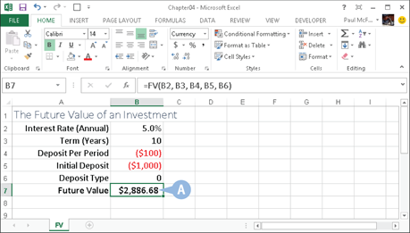
A Excel calculates the future value.
Calculate Present Value
Investors use the concept of present value to recognize the time value of money. Because an investor can receive interest, $1,000 today is worth less than $1,000 ten years from today. For example, $1,000 invested today at 10 percent interest per year, compounded annually, would return $2,593.74. Therefore, the present value of $2,593.74 at 10 percent, compounded annually, for 10 years is $1,000, or worded differently, $1,000 today is worth $2,593.74 ten years from today.
To find the present value, you can use the Excel PV function, which takes five arguments: rate, the interest rate; nper, the number of periods in the term; pmt, the amount of each payment; pv, the amount you are trying to find the present value of; and type, a number indicating when payments are made.
Calculate Present Value
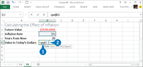
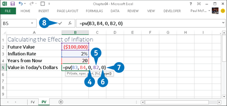
![]() In the cell where you want the present value to appear, type =pv(.
In the cell where you want the present value to appear, type =pv(.
![]() Type the interest rate.
Type the interest rate.

![]() Type a comma and then the number of periods in the term.
Type a comma and then the number of periods in the term.
![]() Type a comma and then the amount of each payment.
Type a comma and then the amount of each payment.
![]() Type a comma and then the future value.
Type a comma and then the future value.
![]() If you need to specify the deposit type, type a comma and then 10 or 1.
If you need to specify the deposit type, type a comma and then 10 or 1.
![]() Type 20.
Type 20.
![]() Click the Enter button or press Enter.
Click the Enter button or press Enter.
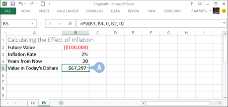
A Excel calculates the present value.
Determine the Loan Payments
When borrowing money, whether it is for a mortgage, car financing, or a student loan, the most basic analysis is to calculate the regular payment you must make to repay the loan. You use the Excel PMT function to determine the payment.
The PMT function takes three required arguments and two optional ones. The required arguments are rate, the fixed rate of interest over the term of the loan; nper, the number of payments over the term of the loan; and pv, the loan principal. The two optional arguments are fv, the future value of the loan, which is usually an end-of-loan balloon payment; and type, the type of payment: 0 (the default) for end-of-period payments or 1 for beginning-of-period payments.
Determine the Loan Payments
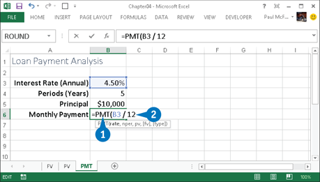
![]() In the cell where you want the payment amount to appear, type =pmt(.
In the cell where you want the payment amount to appear, type =pmt(.
![]() Type the interest rate.
Type the interest rate.
Note: As shown here, if the interest rate is annual, you can divide it by 12 to get the monthly rate.
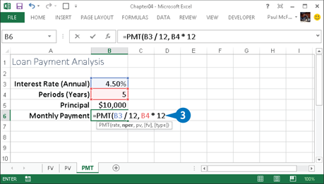
![]() Type a comma and then the number of periods in the term.
Type a comma and then the number of periods in the term.
Note: As shown here, if the term is expressed in years, you can multiply it by 12 to get the number of months in the term.
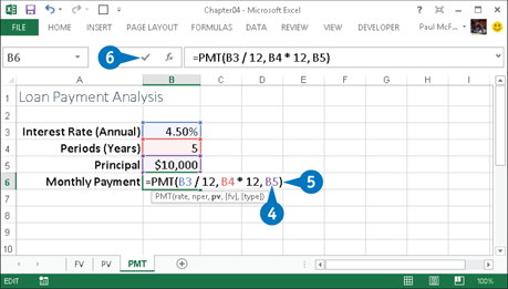
![]() Type a comma and then the amount of the loan principal.
Type a comma and then the amount of the loan principal.
If the loan has a balloon payment, type a comma and then the amount of that payment.
Note: A balloon payment covers any unpaid principal that remains at the end of a loan.
If you need to specify the payment type, type a comma and then 10 or 1.
![]() Type 20.
Type 20.
![]() Click the Enter button or press Enter.
Click the Enter button or press Enter.
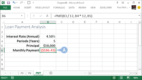
A Excel calculates the loan payment.
Note: The PMT function returns a negative value because it is money that you pay out.
Calculate the Principal or Interest
To break down a loan payment into principal and interest, you can use the PPMT and IPMT functions, respectively. As the loan progresses, the value of PPMT increases while the value of IPMT decreases, but the sum of the two is constant in each period and is equal to the loan payment.
Both functions take the same six arguments. The four required arguments are rate, the fixed rate of interest over the loan term; per, the number of the payment period; nper, the number of payments over the term of the loan; and pv, the loan principal. The two optional arguments are fv, the future value of the loan; and type, the type of payment: 0 for end-of-period or 1 for beginning-of-period.
Calculate the Principal or Interest
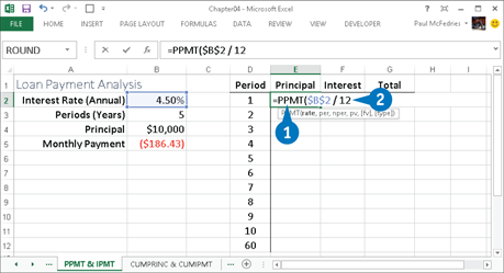
![]() In the cell where you want the principal amount to appear, type =ppmt(.
In the cell where you want the principal amount to appear, type =ppmt(.
![]() Type the interest rate.
Type the interest rate.
Note: As shown here, if you will be filling the calculation into other cells, enter the interest rate address using the absolute reference format.

![]() Type a comma and then the payment period.
Type a comma and then the payment period.
![]() Type a comma and then the number of periods in the term.
Type a comma and then the number of periods in the term.
Note: As shown here, if you will be filling the calculation into other cells, enter the term address using the absolute reference format.
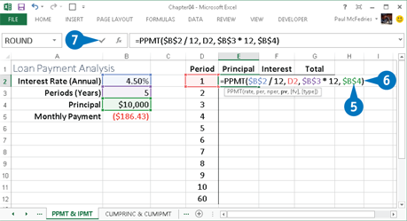
![]() Type a comma and then the amount of the loan principal.
Type a comma and then the amount of the loan principal.
If the loan has a balloon payment, type a comma and then the amount of that payment.
If you need to specify the payment type, type a comma and then 10 or 1.
![]() Type 20.
Type 20.
![]() Click the Enter button or press Enter.
Click the Enter button or press Enter.
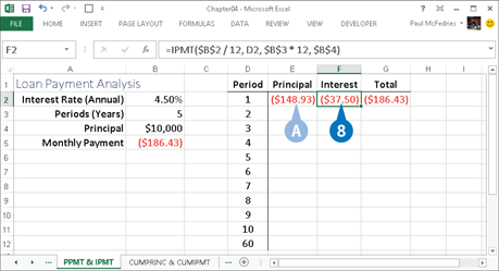
A Excel calculates the principal.
![]() To calculate the interest, type =ipmt( in the cell and then follow steps 2 to 9.
To calculate the interest, type =ipmt( in the cell and then follow steps 2 to 9.
Find the Required Interest Rate
If you know how much you want to borrow, how long a term you want, and what payments you can afford, you can calculate what interest rate will satisfy these parameters using the Excel RATE function. For example, you could use this calculation to put off borrowing money if current interest rates are higher than the value you calculate.
The RATE function takes three required arguments: nper, the number of payments over the term of the loan; pmt, the periodic payment; and pv, the loan principal. RATE can also take three optional arguments: fv, the future value of the loan; type, the type of payment (0 for end-of-period or 1 for beginning-of-period); and guess, a percentage value that Excel uses as a starting point for calculating the interest rate.
Find the Required Interest Rate
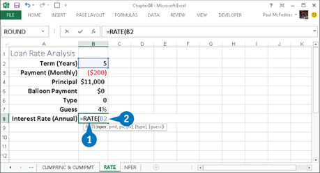
![]() In the cell where you want the interest rate to appear, type =rate(.
In the cell where you want the interest rate to appear, type =rate(.
![]() Type the number of loan periods.
Type the number of loan periods.
Note: If you want an annual interest rate, you must divide the term by 12 if it is currently expressed in months.

![]() Type a comma and then the payment.
Type a comma and then the payment.
Note: As shown here, if you have a monthly payment and you want an annual interest rate, you must multiply the payment by 12.
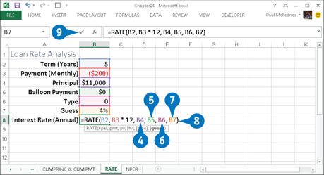
![]() Type a comma and then the amount of the loan principal.
Type a comma and then the amount of the loan principal.
![]() If the loan has a balloon payment, type a comma and then the amount of that payment.
If the loan has a balloon payment, type a comma and then the amount of that payment.
![]() If you need to specify the payment type, type a comma and then 10 or 1.
If you need to specify the payment type, type a comma and then 10 or 1.
![]() If you want to supply an initial guess, type a comma and then specify the value.
If you want to supply an initial guess, type a comma and then specify the value.
![]() Type 20.
Type 20.
![]() Click the Enter button or press Enter.
Click the Enter button or press Enter.

A Excel calculates the interest rate.
Determine the Internal Rate of Return
You can use the Excel IRR function to calculate the internal rate of return on an investment. The investment’s cash flows do not have to be equal, but they must occur at regular intervals. IRR tells you the interest rate you receive on the investment.
IRR takes two arguments values and guess. The values argument is required. It represents the range of cash flows over the term of the investment. It must contain at least one positive and one negative value. The guess argument is optional. It specifies an initial estimate for the Excel iterative calculation of the internal rate of return (the default is 0.1). If after 20 tries Excel cannot return a value, it returns a #NUM! error. You should enter a guess value and try again.
Determine the Internal Rate of Return

![]() Type the series of projected cash flows into a worksheet.
Type the series of projected cash flows into a worksheet.

![]() In the cell where you want the internal rate of return to appear, type =irr(.
In the cell where you want the internal rate of return to appear, type =irr(.

![]() Type the address of the range of cash flows.
Type the address of the range of cash flows.
![]() If you want to supply an initial guess, type a comma and then specify the value.
If you want to supply an initial guess, type a comma and then specify the value.
![]() Type 20.
Type 20.
![]() Click the Enter button or press Enter.
Click the Enter button or press Enter.
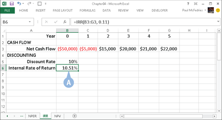
A Excel calculates the internal rate of return.
Calculate Straight-Line Depreciation
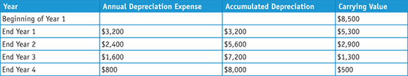
The straight-line method of depreciation allocates depreciation evenly over the useful life of an asset. Salvage value is the value of an asset once its useful life has expired. To calculate straight-line depreciation, you take the cost of the asset, subtract any salvage value, and then divide by the useful life of the asset. The result is the amount of depreciation allocated to each period.
To calculate straight-line depreciation, you can use the Excel SLN function, which takes three arguments: cost, the initial cost of the asset; salvage, the salvage value of the asset; and life, the life of the asset in periods. If you purchase an asset mid-year, you can calculate depreciation in months instead of years.
Calculate Straight-Line Depreciation

![]() In the cell where you want the depreciation amount to appear, type =sln(.
In the cell where you want the depreciation amount to appear, type =sln(.
![]() Type the cost of the asset.
Type the cost of the asset.

![]() Type a comma and then the salvage value of the asset.
Type a comma and then the salvage value of the asset.

![]() Type a comma and then the number of periods in the useful life of the asset.
Type a comma and then the number of periods in the useful life of the asset.
![]() Type 20.
Type 20.
![]() Click the Enter button or press Enter.
Click the Enter button or press Enter.
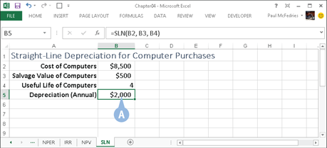
A Excel calculates the straight-line depreciation.
APPLY IT
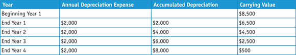
The carrying value is the cost of an asset minus the total depreciation taken to date. The depreciation for an asset with a cost of $8,500, a salvage value of $500, and a useful life of four years would be allocated as follows:
Return the Fixed-Declining Balance Depreciation
When calculating depreciation, accountants try to match the cost of an asset with the revenue it produces. Some assets produce more in earlier years than in later years. For those assets, accountants use accelerated methods of depreciation, which take more depreciation in the earlier years than in the later years. Fixed-declining balance is an accelerated method of depreciation.
To calculate fixed-declining balance depreciation, you can use the Excel DB function, which takes five arguments: cost, the cost of the asset; salvage, the salvage value; life, the useful life; period, the period for which you are calculating depreciation; and the optional month, the number of months in the first year. If you leave month blank, Excel uses a default value of 12.
Return the Fixed-Declining Balance Depreciation
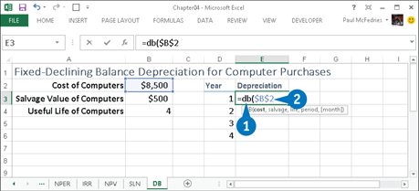
![]() In the cell where you want the depreciation amount to appear, type =db(.
In the cell where you want the depreciation amount to appear, type =db(.
![]() Type the cost of the asset.
Type the cost of the asset.
Note: As shown here, if you will be filling the calculation into other cells, enter the cost address using the absolute reference format.

![]() Type a comma and then the salvage value of the asset.
Type a comma and then the salvage value of the asset.
![]() Type a comma and then the number of periods in the useful life of the asset.
Type a comma and then the number of periods in the useful life of the asset.
Note: As shown here, if you will be filling the calculation into other cells, enter the salvage and life addresses using the absolute reference format.

![]() Type a comma and then the type of period for which you are calculating the depreciation.
Type a comma and then the type of period for which you are calculating the depreciation.
If the number of months in the first year is different than 12, type a comma and then type the number of months in the first year.
![]() Type 20.
Type 20.
![]() Click the Enter button or press Enter.
Click the Enter button or press Enter.

A Excel calculates the fixed-declining balance depreciation.
APPLY IT
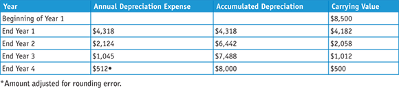
The fixed-declining balance method of depreciation depreciates an asset with a cost of $8,500, a salvage value of $500, and a useful life of four years as follows:
Determine the Double-Declining Balance Depreciation
Double-declining balance is an accelerated depreciation method that takes the rate you would apply by using straight-line depreciation, doubles it, and then applies the doubled rate to the carrying value of the asset. To determine the double-declining balance depreciation, you can use the Excel DDB function, which takes five arguments: cost, the cost of the asset; salvage, the salvage value; life, the useful life; period, the period for which you are calculating depreciation; and the optional factor, the rate at which the balance declines. The default value for factor is 2, but to use a value other than twice the straight-line rate, you can enter the factor you want to use, such as 1.5 for a rate of 150 percent.
Determine the Double-Declining Balance Depreciation

![]() In the cell where you want the depreciation amount to appear, type =ddb(.
In the cell where you want the depreciation amount to appear, type =ddb(.
![]() Type the cost of the asset.
Type the cost of the asset.
Note: As shown here, if you will be filling the calculation into other cells, enter the cost address using the absolute reference format.
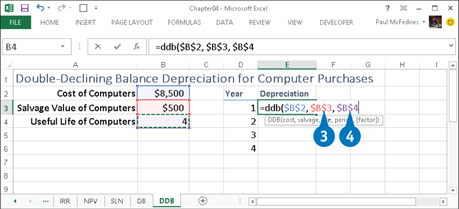
![]() Type a comma and then the salvage value of the asset.
Type a comma and then the salvage value of the asset.
![]() Type a comma and then the number of periods in the useful life of the asset.
Type a comma and then the number of periods in the useful life of the asset.
Note: As shown here, if you will be filling the calculation into other cells, enter the salvage and life addresses using the absolute reference format.

![]() Type a comma and then the type of period for which you are calculating the depreciation.
Type a comma and then the type of period for which you are calculating the depreciation.
If you want to use a rate other than 2, type a comma and then type the factor value you want to use.
![]() Type 20.
Type 20.
![]() Click the Enter button or press Enter.
Click the Enter button or press Enter.
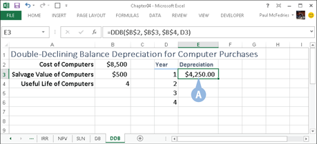
A Excel calculates the double-declining balance depreciation.
APPLY IT
The double-declining balance method of depreciation depreciates an asset with a cost of $8,500, a salvage value of $1,500, and a useful life of four years as follows:
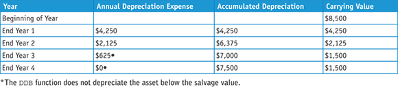
*The DDB function does not depreciate the asset below the salvage value.
Figure the Sum-of-the-Years-Digits Depreciation
Sum-of-the-years-digits is an accelerated depreciation method. When you calculate sum-of-the-years-digits depreciation manually, you use a fraction to calculate annual depreciation. The numerator of the fraction is the remaining years of useful life. The denominator is the sum of the digits that make up the useful life.
To determine the sum-of-the-years-digits depreciation, you can use the Excel SYD function, which takes four arguments. The cost argument is the cost of the asset. The salvage argument is the salvage value. The life argument is the useful life. The per argument is the period for which you are calculating depreciation.
Figure the Sum-of-the-Years-Digits Depreciation
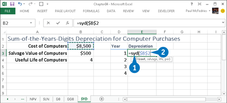
![]() In the cell where you want the depreciation amount to appear, type =syd(.
In the cell where you want the depreciation amount to appear, type =syd(.
![]() Type the cost of the asset.
Type the cost of the asset.
Note: As shown here, if you will be filling the calculation into other cells, enter the cost address using the absolute reference format.

![]() Type a comma and then the salvage value of the asset.
Type a comma and then the salvage value of the asset.
![]() Type a comma and then the number of periods in the useful life of the asset.
Type a comma and then the number of periods in the useful life of the asset.
Note: As shown here, if you will be filling the calculation into other cells, enter the salvage and life addresses using the absolute reference format.
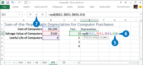
![]() Type a comma and then the type of period for which you are calculating the depreciation.
Type a comma and then the type of period for which you are calculating the depreciation.
![]() Type 20.
Type 20.
![]() Click the Enter button or press Enter.
Click the Enter button or press Enter.

A Excel calculates the sum-of-the-years-digits depreciation.
APPLY IT
The sum-of-the-years-digits method of depreciation depreciates an asset with a cost of $8,500, a salvage value of $500, and a useful life of four years as follows: