
Chapter 12
Analyzing Data with PivotTables
Understanding PivotTables
Tables and external databases can contain thousands of records. Analyzing that much data can be a nightmare without the right kinds of tools. To help, Excel offers a powerful data analysis tool called a PivotTable, which enables you to summarize hundreds of records in a concise tabular format. You can then manipulate the layout of — or pivot — the table to see different views of your data.
PivotTables help you analyze large amounts of data by performing three operations: grouping the data into categories, summarizing the data using calculations, and filtering the data to show just the records you want to work with.
Grouping
A PivotTable is a powerful data-analysis tool in part because it automatically groups large amounts of data into smaller, more manageable categories. For example, suppose you have a data source with a Region field where each cell contains one of four values: East, West, North, and South. The original data may contain thousands of records, but if you build your PivotTable using the Region field, the resulting table has just four rows — one each for the four unique Region values in your data.
You can also create your own grouping after you build your PivotTable. For example, if your data has a Country field, you can build the PivotTable to group together all the records that have the same Country value. When you have done that, you can further group the unique Country values into continents: North America, South America, Europe, and so on.
Summarizing
In conjunction with grouping data according to the unique values in one or more fields, Excel also displays summary calculations for each group. The default calculation is Sum, which means for each group, Excel totals all the values in some specified field. For example, if your data has a Region field and a Sales field, a PivotTable can group the unique Region values and display the total of the Sales values for each one. Excel has other summary calculations, including Count, Average, Maximum, Minimum, and Standard Deviation.
Even more powerful, a PivotTable can display summaries for one grouping broken down by another. For example, suppose your sales data also has a Product field. You can set up a PivotTable to show the total Sales for each Product, broken down by Region.
Filtering
A PivotTable also enables you to view just a subset of the data. For example, by default the PivotTable’s groupings show all the unique values in the field. However, you can manipulate each grouping to hide those that you do not want to view. Each PivotTable also comes with a report filter that enables you to apply a filter to the entire PivotTable. For example, suppose your sales data also includes a Customer field. By placing this field in the PivotTable’s report filter, you can filter the PivotTable report to show just the results for a single Customer.
Explore PivotTable Features
PivotTables are worth learning about because they come with a long list of benefits. For example, PivotTables are easy to build and maintain, and they perform large and complex calculations amazingly fast. You can update PivotTables quickly and easily to account for new data. Because they are dynamic, you can easily move, filter, and add components. PivotTables are fully customizable so you can build each report the way you want, and they can use most of the formatting options that you can apply to regular Excel ranges.
You can get up to speed with PivotTables very quickly after you learn a few key concepts. You need to understand the features that make up a typical PivotTable, particularly the four areas — row, column, data, and filter — to which you add fields from your data.
Get Familiar with PivotTable Features
A Filter
Displays a drop-down list that contains the unique values from a field. When you select a value from the list, Excel filters the PivotTable results to include only the records that match the selected value.
B Column Area
Displays horizontally the unique values from a field in your data.
C Row Area
Displays vertically the unique values from a field in your data.
D Data Area
Displays the results of the calculation that Excel applied to a numeric field in your data.
E Row Field Header
Identifies the field contained in the row area. You also use the row field header to filter the field values that appear in the row area.
F Column Field Header
Identifies the field contained in the column area. You also use the column field header to filter the field values that appear in the column area.
G Data Field Header
Specifies both the calculation (such as Sum) and the field (such as Invoice Total) used in the data area.
H Field Items
Consists of the unique values for the field added to the particular area.

Build a PivotTable from an Excel Range or Table
If the data you want to analyze exists as an Excel range or table, you can use the PivotTable command to easily build a PivotTable report based on your data. You need only specify the location of your source data and then choose the location of the resulting PivotTable.
Excel creates an empty PivotTable in a new worksheet or in the location you specified. Excel also displays the PivotTable Fields pane, which contains four areas: FILTERS, COLUMNS, ROWS, and VALUES. To complete the PivotTable, you must populate some or all of these areas with one or more fields from your data.
Build a PivotTable from an Excel Range or Table

![]() Click a cell within the range or table that you want to use as the source data.
Click a cell within the range or table that you want to use as the source data.
![]() Click the Insert tab.
Click the Insert tab.
![]() Click PivotTable.
Click PivotTable.

The Create PivotTable dialog box appears.
![]() Click the New Worksheet option (
Click the New Worksheet option (![]() changes to
changes to ![]() ).
).
A If you want to place the PivotTable in an existing location, click the Existing Worksheet option (![]() changes to
changes to ![]() ) and then use the Location range box to select the worksheet and cell where you want the PivotTable to appear.
) and then use the Location range box to select the worksheet and cell where you want the PivotTable to appear.
![]() Click OK.
Click OK.

B Excel creates a blank PivotTable.
C Excel displays the PivotTable Fields pane.
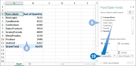
![]() Click and drag a field and drop it inside the ROWS area.
Click and drag a field and drop it inside the ROWS area.
D Excel adds the field’s unique values to the PivotTable’s row area.
![]() Click and drag a numeric field and drop it inside the VALUES area.
Click and drag a numeric field and drop it inside the VALUES area.
E Excel sums the numeric values based on the row values.
![]() If desired, click and drag fields and drop them in the COLUMNS area and the FILTERS area.
If desired, click and drag fields and drop them in the COLUMNS area and the FILTERS area.
Each time you drop a field in an area, Excel updates the PivotTable to include the new data.
EXTRA
Excel offers a few shortcut techniques for building PivotTables. In the PivotTable Fields pane, click a check box for a text or date field (![]() changes to
changes to ![]() ) to add it to the ROWS area; click a check box for a numeric field (
) to add it to the ROWS area; click a check box for a numeric field (![]() changes to
changes to ![]() ) to add it to the VALUES area. You can also right-click a field and then click the area that you want to use. You use the FILTERS box to add a filter field to the PivotTable, which enables you to display a subset of the data based on an item from that field. Click the down arrow in the filter field, select the item that you want to use as a filter from the drop-down list, and then click OK.
) to add it to the VALUES area. You can also right-click a field and then click the area that you want to use. You use the FILTERS box to add a filter field to the PivotTable, which enables you to display a subset of the data based on an item from that field. Click the down arrow in the filter field, select the item that you want to use as a filter from the drop-down list, and then click OK.
Create a PivotTable from External Data
Rather than creating a PivotTable from data within an Excel worksheet, you may want to create a PivotTable using an external data source. This enables you to build reports from extremely large datasets and from relational database systems.
The data you are analyzing might not exist in an Excel range or table, but outside of Excel in a relational database management system (RDBMS) such as Microsoft Access or SQL Server. With these programs, you can set up a table, query, or other object that defines the data you want to work with. You can then build your PivotTable based on this external data source.
Create a PivotTable from External Data
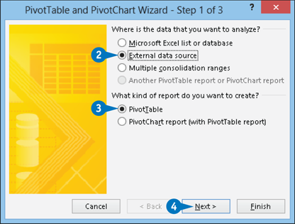
![]() Press Alt+D and then press P.
Press Alt+D and then press P.
The PivotTable and PivotChart Wizard - Step 1 of 3 dialog box appears.
![]() Click the External Data Source option (
Click the External Data Source option (![]() changes to
changes to ![]() ).
).
![]() Click the PivotTable option (
Click the PivotTable option (![]() changes to
changes to ![]() ).
).
![]() Click Next.
Click Next.
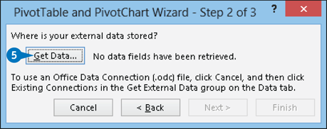
The PivotTable and PivotChart Wizard - Step 2 of 3 dialog box appears.
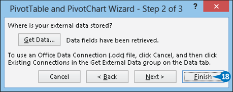
![]() Click Get Data.
Click Get Data.
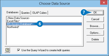
The Choose Data Source dialog box appears.
![]() Click the type of data source you want to use.
Click the type of data source you want to use.
![]() Click OK.
Click OK.
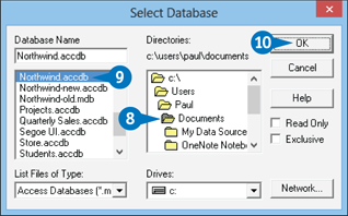
The Select Database dialog box appears.
![]() Click the folder that contains the database.
Click the folder that contains the database.
![]() Click the database.
Click the database.
![]() Click OK.
Click OK.
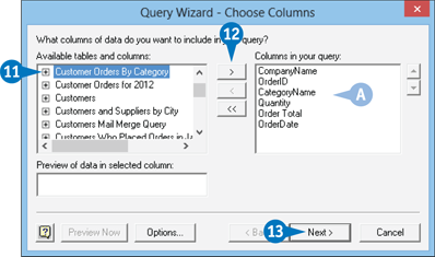
The Query Wizard - Choose Columns dialog box appears.
![]() Click the table or column you want to use as the source data for your PivotTable.
Click the table or column you want to use as the source data for your PivotTable.
![]() Click Add.
Click Add.
A The table’s fields appear in this list.
![]() Click Next.
Click Next.
EXTRA
To create a data source, click the Excel Data tab, click Get External Data, click From Other Sources, and then click From Microsoft Query. In the Choose Data Source dialog box, click New Data Source. Click to deselect the Use the Query Wizard to Create/Edit Queries check box (![]() changes to
changes to ![]() ), and then click OK. In the Create New Data Source dialog box, type a name for your data source, select the database driver that your data source requires, and then click OK.
), and then click OK. In the Create New Data Source dialog box, type a name for your data source, select the database driver that your data source requires, and then click OK.
When you create a PivotTable from external data, you need to have already defined the appropriate data source. Note, as well, that you do not need to work with Microsoft Query directly. Note, too, that when you create a PivotTable from external data, you can skip over the Query Wizard dialog boxes that enable you to filter and sort the external data, because this is not usually pertinent for a PivotTable.
When you create a PivotTable from external data, you do not need the external data to be imported to Excel. Rather, the external data resides only in the new PivotTable; you do not see the actual data in your workbook.
Create a PivotTable from External Data
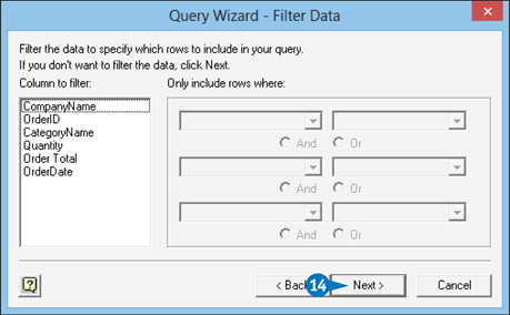
The Query Wizard - Filter Data dialog box appears.
![]() Click Next.
Click Next.
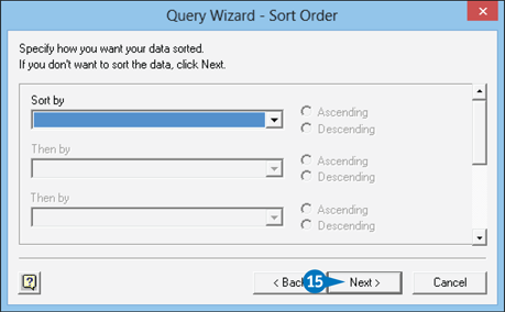
The Query Wizard - Sort Order dialog box appears.
![]() Click Next.
Click Next.

The Query Wizard - Finish dialog box appears.
![]() Click the Return Data to Microsoft Excel options (
Click the Return Data to Microsoft Excel options (![]() changes to
changes to ![]() ).
).
![]() Click Finish.
Click Finish.
Excel returns you to the PivotTable and PivotChart Wizard - Step 2 of 3 dialog box.
![]() Click Finish.
Click Finish.
Excel creates an empty PivotTable.
A The fields available in the table or query that you chose in step 11 appear in the PivotTable Fields pane.
![]() Click and drag fields from the PivotTable Fields pane and drop them in the PivotTable areas.
Click and drag fields from the PivotTable Fields pane and drop them in the PivotTable areas.
B Excel summarizes the external data in the PivotTable.
Refresh PivotTable Data
Whether your PivotTable is based on financial results, survey responses, or a database of collectibles such as books or DVDs, the underlying data is probably not static. That is, the data changes over time as new results come in, new surveys are undertaken, and new items are added to the collection. You can ensure that the data analysis represented by the PivotTable remains up to date by refreshing the PivotTable.
Excel offers two methods for refreshing a PivotTable: manual and automatic. A manual refresh is one that you perform, usually when you know that the source data has changed, or if you simply want to be sure that the latest data is reflected in your PivotTable report. An automatic refresh is one that Excel handles for you.
Refresh PivotTable Data
Refresh Data Manually

![]() Click any cell inside the PivotTable.
Click any cell inside the PivotTable.
![]() Click the Analyze tab.
Click the Analyze tab.
![]() Click Refresh.
Click Refresh.
You can also press Alt+F5.
A To update every PivotTable in the workbook, click the Refresh down arrow and then click Refresh All.
You can also update all PivotTables by pressing Ctrl+Alt+F5.
Excel updates the PivotTable data.
Refresh Data Automatically
![]() Click any cell inside the PivotTable.
Click any cell inside the PivotTable.
![]() Click the Analyze tab.
Click the Analyze tab.
![]() Click PivotTable.
Click PivotTable.
![]() Click Options.
Click Options.
Note: You can also right-click any cell in the PivotTable and then click PivotTable Options.

The PivotTable Options dialog box appears.
![]() Click the Data tab.
Click the Data tab.
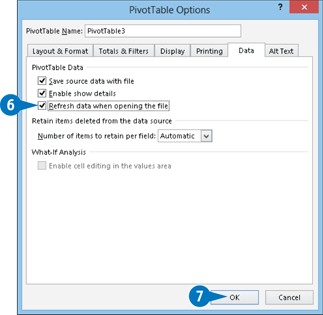
![]() Click the Refresh Data When Opening the File check box (
Click the Refresh Data When Opening the File check box (![]() changes to
changes to ![]() ).
).
![]() Click OK.
Click OK.
Excel applies the refresh options.
APPLY IT
If your PivotTable is based on external data, you can set up a schedule that automatically refreshes the PivotTable at a specified interval. Click any cell inside the PivotTable, click the Analyze tab, click the Refresh down arrow, and then select Connection Properties from the drop-down list. Click the Refresh Every check box (![]() changes to
changes to ![]() ), and then use the spin box to specify the refresh interval, in minutes.
), and then use the spin box to specify the refresh interval, in minutes.
Note, however, that when you set up an automatic refresh, you might prefer not to have the source data updated too frequently. Depending on where the data resides and how much data you are working with, the refresh could take some time, which may slow down the rest of your work.
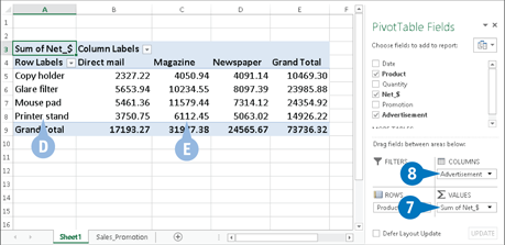
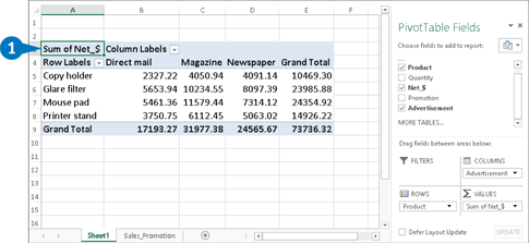
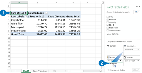
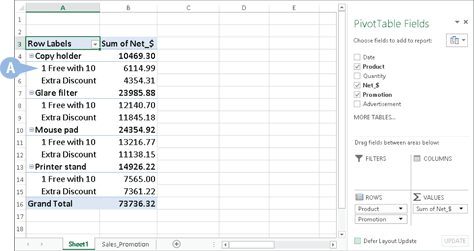
Add Multiple Fields to the Row or Column Area
You can add multiple fields to any of the PivotTable areas. This powerful feature enables you to perform further analysis of your data by viewing the data differently. For example, suppose that you are analyzing the results of a sales campaign that ran different promotions in several types of advertisements. A basic PivotTable might show you the sales for each Product (the row field) according to the Advertisement used (the column field). You might also be interested in seeing, for each product, the breakdown in sales for each promotion. You can do that by adding the Promotion field to the row area.
Add Multiple Fields to the Row or Column Area
Add a Field to the ROWS Area
![]() Click a cell within the PivotTable.
Click a cell within the PivotTable.

![]() Click the check box of the text or date field that you want to add (
Click the check box of the text or date field that you want to add (![]() changes to
changes to ![]() ).
).
A Excel adds the field to the ROWS box.
B Excel adds the field’s unique values to the PivotTable’s row area.
Add a Field to the ROWS or COLUMNS Area

![]() Click a cell within the PivotTable.
Click a cell within the PivotTable.
![]() From the list in the PivotTable Fields pane, click and drag the field that you want to add and drop the field in either the ROWS box or the COLUMNS box.
From the list in the PivotTable Fields pane, click and drag the field that you want to add and drop the field in either the ROWS box or the COLUMNS box.

C Excel adds the field to the ROWS or COLUMNS box.
D Excel adds the field’s unique values to the PivotTable’s row or column area.
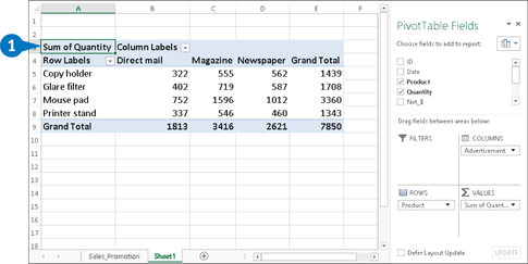
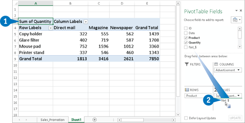
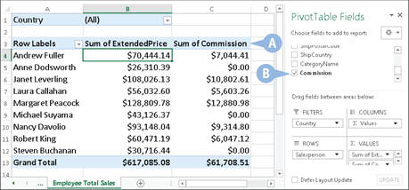
Add Multiple Fields to the Data Area
Excel enables you to add multiple fields to the PivotTable’s data area, which enhances your analysis by enabling you to see multiple summaries at one time. For example, suppose you are analyzing the results of a sales campaign. A basic PivotTable might show you the sum of the quantity sold. You might also be interested in seeing the net dollar amount sold. You can do that by adding the Net $ field to the data area. You can add multiple fields to the data area either by using the PivotTable Fields pane or by dragging a field to the data area.
Add Multiple Fields to the Data Area
Add a Field to the Data Area with a Check Box
![]() Click a cell within the PivotTable.
Click a cell within the PivotTable.

![]() Select the check box of the field you want to add to the data area.
Select the check box of the field you want to add to the data area.
A Excel adds a button for the field to the VALUES box.
B Excel adds the field to the PivotTable’s data area.
Add a Field to the Data Area by Dragging
![]() Click a cell within the PivotTable.
Click a cell within the PivotTable.
![]() In the PivotTable Fields pane, click and drag the field you want to add and drop the field in the VALUES box.
In the PivotTable Fields pane, click and drag the field you want to add and drop the field in the VALUES box.

C Excel adds the field to the PivotTable’s data area.
Move a Field to a Different Area
A PivotTable is a powerful data analysis tool because it can take hundreds or even thousands of records and summarize them into a compact, comprehensible report. However, unlike most of the other data-analysis features in Excel, a PivotTable is not a static collection of worksheet cells. Instead, you can move a PivotTable’s fields from one area of the PivotTable to another. This enables you to view your data from different perspectives, which can greatly enhance the analysis of the data. Moving a field within a PivotTable is called pivoting the data.
The most common way to pivot the data is to move fields between the row and column areas. However, you can also pivot data by moving a row or column field to the filter area.
Move a Field to a Different Area
Move a Field between the Row and Column Areas
![]() Click a cell within the PivotTable.
Click a cell within the PivotTable.
![]() Click and drag a COLUMNS field button and drop it within the ROWS box.
Click and drag a COLUMNS field button and drop it within the ROWS box.
A Excel displays the field’s values within the row area.
You can also drag a field button from the ROWS box area and drop it within the COLUMNS box.
Move a Row or Column Field to the Filters Area

![]() Click a cell within the PivotTable.
Click a cell within the PivotTable.
![]() Click and drag a field from the ROWS box and drop it within the FILTERS box.
Click and drag a field from the ROWS box and drop it within the FILTERS box.
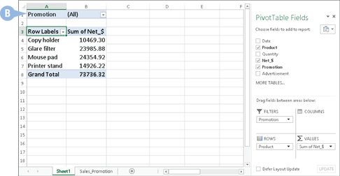
B Excel moves the field button to the report filter.
You can also drag a field button from the COLUMNS box and drop it within the FILTERS box.
Group PivotTable Values
To make a PivotTable with a large number of row or column items easier to work with, you can group the items together. For example, you could group months into quarters, thus reducing the number of items from twelve to four. Similarly, a report that lists dozens of countries could group those countries by continent, thus reducing the number of items to four or five, depending on where the countries are located. Finally, if you use a numeric field in the row or column area, you may have hundreds of items, one for each numeric value. You can improve the report by creating just a few numeric ranges.
Group PivotTable Values
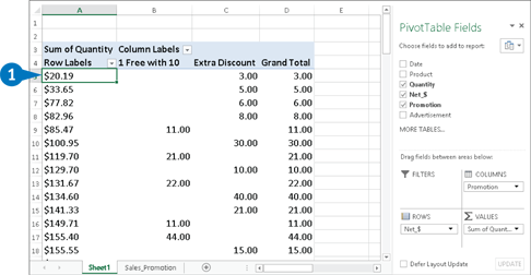
![]() Click any item in the numeric field that you want to group.
Click any item in the numeric field that you want to group.

![]() Click the Analyze tab.
Click the Analyze tab.
![]() Click Group.
Click Group.
![]() Click Group Field.
Click Group Field.
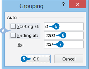
The Grouping dialog box appears.
![]() Type the starting numeric value.
Type the starting numeric value.
A Click these check boxes (![]() changes to
changes to ![]() ) to have Excel extract the minimum and maximum values of the numeric items and place those values in the text boxes.
) to have Excel extract the minimum and maximum values of the numeric items and place those values in the text boxes.
![]() Type the ending numeric value.
Type the ending numeric value.
![]() Type the size that you want to use for each grouping.
Type the size that you want to use for each grouping.
![]() Click OK.
Click OK.

B Excel groups the numeric values.
Change the PivotTable Summary Calculation
If your data analysis requires a calculation other than Sum (for numeric data) or Count (for text), you can configure the data field to use any one of the nine other summary calculations that are built into Excel. For example, Average calculates the mean value in a numeric field. Max and Min display the largest and smallest value, respectively, in a numeric field. Product multiplies the values in a numeric field, while Count Nums displays the total number of numeric values in the source field. StdDev and StdDevp calculate the standard deviation of a population sample and entire population, respectively. Var and Varp calculate the variance of a population sample and entire population, respectively.
Change the PivotTable Summary Calculation

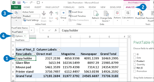
![]() Click any cell in the data field.
Click any cell in the data field.

![]() Click the Analyze tab.
Click the Analyze tab.
![]() Click Active Field.
Click Active Field.
![]() Click Field Settings.
Click Field Settings.
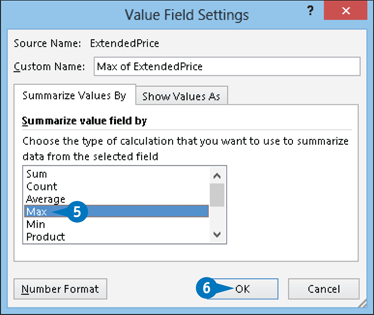
The Value Field Settings dialog box appears with the Summarize Values By tab displayed.
![]() Click the summary calculation you want to use.
Click the summary calculation you want to use.
![]() Click OK.
Click OK.
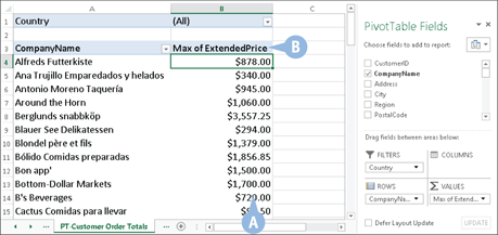
A Excel recalculates the PivotTable results.
B Excel renames the data field label to reflect the new summary calculation.
EXTRA
If your PivotTable results do not look correct, check the summary calculation that Excel has applied to the field to see if it is using Count instead of Sum. If the data field includes one or more text cells or one or more blank cells, Excel defaults to the Count summary function instead of Sum. When you add a second field to the row or column area, Excel displays a subtotal for each item in the outer field. To change the subtotal summary calculation, click any cell in the outer field, click the Analyze tab, click Active Field, and then click Field Settings. Select the Custom option (![]() changes to
changes to ![]() ), and then click the summary calculation you want to use for the subtotals. Click OK.
), and then click the summary calculation you want to use for the subtotals. Click OK.
Introducing Custom Calculations
A custom calculation is a formula that you define to produce PivotTable values that would not otherwise appear in the report if you used only the source data fields and the built-in summary calculations in Excel. Custom calculations enable you to extend your data analysis to include results that are specific to your needs.
For example, suppose your PivotTable shows employee sales by quarter and you want to award a 10-percent bonus to each employee with sales of more than $25,000 in any quarter. You can create a custom calculation that checks for sales greater than $25,000 and then multiplies them by 0.1 to get the bonus number.
Excel applies a custom calculation to your source data to produce a summary result. In most cases, the custom calculation is just like the PivotTable summary calculations that are built into Excel, except that you define the specifics of the calculation. Because you are creating a formula, you can use most of the formula power available in Excel, which gives you tremendous flexibility to create custom calculations that suit your data-analysis needs. By placing these calculations within the actual PivotTable, as opposed to adding them to your source data, you can easily update the calculations as needed and refresh the report results.
Custom Calculation Types
When building a custom calculation for a PivotTable, Excel offers two types: a calculated field and a calculated item.
Calculated Field
If your data analysis requires a PivotTable field that is not available from the data source or via Excel’s built-in summary calculations, you can insert a custom formula to derive the field you need. A calculated field is a new data field in which the values are the result of a custom calculation formula. You can display the calculated field along with another data field or on its own. A calculated field is really a custom summary calculation, so in almost all cases, the calculated field references one or more fields in the source data. For more information, see the Insert a Custom Calculated Field section later in this chapter.
Calculated Item
If your data analysis requires a PivotTable item that is not available from the data source or via Excel’s built-in summary calculations, you can insert a custom formula to derive the item you need. A calculated item is a new item in a row or column field in which the values are the result of a custom calculation. In this case, the calculated item’s formula references one or more items in the same field.
Understanding Custom Calculation Limitations
Whether they are calculated fields or calculated items, custom calculations are powerful additions to your PivotTable analysis toolbox. However, although custom calculation formulas look like regular worksheet formulas, you cannot assume that you can do everything with a custom PivotTable formula that you can do with a worksheet formula. In fact, there are a number of limitations that Excel imposes on custom formulas, such as not being able to reference data outside the pivot cache, and not being able to use custom items in conjunction with grouping.
General Limitations
The major limitation inherent in custom calculations is that, with the exception of constant values such as numbers, you cannot reference anything outside the PivotTable’s source data:
• You cannot use a cell reference, range address, or range name as an operand in a custom calculation formula.
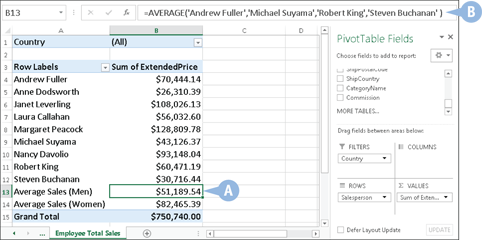
• You cannot use any worksheet function that requires a cell reference, range, or defined name. However, you can still use many of the Excel worksheet functions by substituting either a field or an item in place of a cell reference or range name. For example, if you want a calculated item that returns the average of items named Jan, Feb, and Mar, you could use the following formula:
=AVERAGE(Jan, Feb, Mar)
• You cannot use the PivotTable’s subtotals, row totals, column totals, or Grand Total as an operand in a custom calculation formula.
Calculated Field Limitations
When you are working with calculated fields, it is important to understand how references to other PivotTable fields work within your calculations and what limitations you face when using field references.
Field References
When you reference a field in your formula, Excel interprets this reference as the sum of that field’s values. For example, the formula =Sales + 1 does not add 1 to each Sales value and return the sum of these results; that is, Excel does not interpret the formula as =Sum of (Sales + 1). Instead, the formula adds 1 to the sum of the Sales values; Excel interprets the formula as =(Sum of Sales) + 1.
Field Reference Problems
The fact that Excel defaults to a Sum calculation when you reference another field in your custom calculation can lead to problems. The trouble is that it does not make sense to sum certain types of data. For example, suppose you have inventory source data with UnitsInStock and UnitPrice fields. You want to calculate the total value of the inventory, so you create a custom field based on the following formula:
=UnitsInStock * UnitPrice
Unfortunately, this formula does not work because Excel treats the UnitPrice operand as Sum of UnitPrice. Of course, it does not make sense to “add” the prices together, so your formula produces an incorrect result.
Calculated Item Limitations
Excel imposes the following limitations on the use of calculated items:
• A formula for a calculated item cannot reference items from any field except the one in which the calculated item resides.
• You cannot insert a calculated item into a PivotTable that has at least one grouped field. You must ungroup all the PivotTable fields before you can insert a calculated item.
• You cannot group a field in a PivotTable that has at least one calculated item.
• You cannot insert a calculated item into a page field. Also, you cannot move a row or column field that has a calculated item into the page area.
• You cannot insert a calculated item into a PivotTable in which a field has been used more than once.
• You cannot insert a calculated item into a PivotTable that uses the Average, StdDev, StdDevp, Var, or Varp summary calculations.
Insert a Custom Calculated Field
If your data analysis requires a PivotTable field that is not available using just the data source fields and the summary calculations that are built into Excel, you can insert a calculated field that uses a custom formula to derive the results you need. A custom calculated field is based on a formula that looks much like an Excel worksheet formula. However, you do not enter the formula for a calculated field into a worksheet cell. Instead, Excel offers the Calculated Field feature, which provides a dialog box for you to name the field and construct the formula. Excel then stores the formula along with the rest of the PivotTable data in the pivot cache.
Insert a Custom Calculated Field

![]() Click any cell inside the PivotTable’s data area.
Click any cell inside the PivotTable’s data area.
![]() Click Analyze.
Click Analyze.
![]() Click Calculations.
Click Calculations.
![]() Click Fields, Items, & Sets.
Click Fields, Items, & Sets.
![]() Click Calculated Field.
Click Calculated Field.
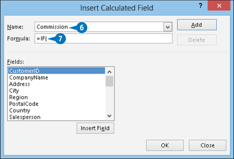
The Insert Calculated Field dialog box appears.
![]() Type a name for the calculated field.
Type a name for the calculated field.
![]() Start the formula for the calculated field.
Start the formula for the calculated field.
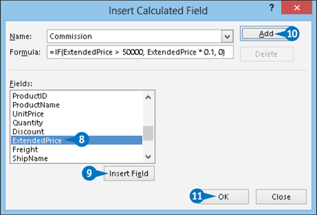
![]() To insert a field into the formula at the current cursor position, click the field.
To insert a field into the formula at the current cursor position, click the field.
![]() Click Insert Field.
Click Insert Field.
![]() When the formula is complete, click Add.
When the formula is complete, click Add.
![]() Click OK.
Click OK.
A Excel adds the calculated field to the PivotTable’s data area.
B Excel adds the calculated field to the PivotTable Fields pane.
Insert a Custom Calculated Item
If your data analysis requires a PivotTable item that is not available using just the data source fields and the summary calculations that are built into Excel, you can insert a calculated item that uses a custom formula to derive the results you need. A calculated item uses a formula much like an Excel worksheet formula. However, you do not enter the formula for a calculated item into a worksheet cell. Instead, Excel offers the Calculated Item command, which displays a dialog box where you name the item and construct the formula. Excel then stores the formula along with the rest of the PivotTable data in the pivot cache. Before you create a calculated item, be sure to remove all groupings from your PivotTable.
Insert a Custom Calculated Item
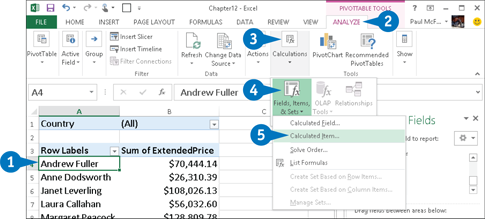
![]() Click any cell inside the field into which you want to insert the item.
Click any cell inside the field into which you want to insert the item.
![]() Click Analyze.
Click Analyze.
![]() Click Calculations.
Click Calculations.
![]() Click Fields, Items, & Sets.
Click Fields, Items, & Sets.
![]() Click Calculated Item.
Click Calculated Item.
The Insert Calculated Item dialog box appears.
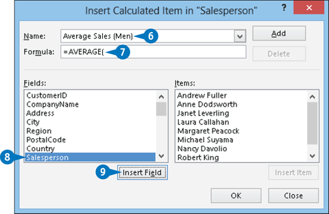
![]() Type a name for the calculated item.
Type a name for the calculated item.
![]() Start the formula for the calculated item.
Start the formula for the calculated item.
![]() To insert a field into the formula at the current cursor position, click the field.
To insert a field into the formula at the current cursor position, click the field.
![]() Click Insert Field.
Click Insert Field.
You can also double-click the field.
![]() To insert an item into the formula at the current cursor position, click the field containing the item.
To insert an item into the formula at the current cursor position, click the field containing the item.
![]() Click the item.
Click the item.
![]() Click Insert Item.
Click Insert Item.
You can also double-click the item.
![]() When the formula is complete, click Add.
When the formula is complete, click Add.
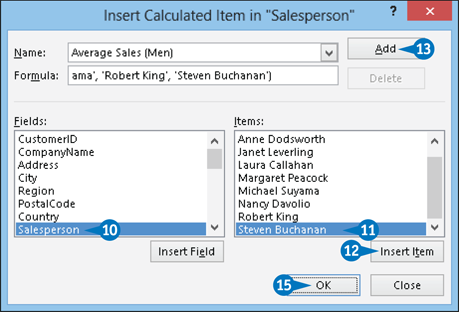
![]() Repeat steps 6 to 13 to add other calculated items.
Repeat steps 6 to 13 to add other calculated items.
![]() Click OK.
Click OK.
A Excel adds the calculated item to the field.
B The calculated item’s formula appears in the Formula bar when you click the result.