Chapter 2

Troubleshooting Formulas

Understanding Error Values in Excel

Excel formula errors fall into three main categories. First, there are the syntax errors, where Excel generates an error message when you press Enter to accept the formula. For example, if you forget a function’s closing parenthesis, Excel displays an error letting you know that the parenthesis is missing. Next, there are the inaccuracy errors, where your worksheet data is wrong, one or more operators or operands in your formula are wrong, or both. Finally, there are the errors where Excel cannot compute a formula result and, instead, displays an error value. Excel has seven different error values — #DIV/0!, #N/A, #NAME?, #NULL!, #NUM!, #REF!, and #VALUE!.

#DIV/0!

The #DIV/0! error usually means that the cell’s formula is trying to divide by zero, which is not allowed. The cause is usually a reference to a cell that either is blank or contains the value 0. Check the cell’s precedents (the cells that are directly or indirectly referenced in the formula) to look for possible culprits. You also see #DIV/0! if you enter an inappropriate argument in some functions. The MOD function, for example, returns #DIV/0! if the second argument is 0.

#N/A

The #N/A error value is short for not available, and it means that the formula could not return a legitimate result. You usually see #N/A when you use an inappropriate argument (or if you omit a required argument) in a function. For example, the HLOOKUP and VLOOKUP functions return #N/A if the lookup value is smaller than the first value in the lookup range.

To solve the problem, first check the formula’s input cells to see if any of them are displaying the #N/A error. If so, that is why your formula is returning the same error; the problem actually lies in the input cell. When you have found where the error originates, examine the formula’s operands to look for inappropriate data types. In particular, check the arguments used in each function to ensure that they make sense for the function and that no required arguments are missing.

#NAME?

The #NAME? error appears when Excel does not recognize a name you used in a formula, or when it interprets text within the formula as an undefined name. This means that the #NAME? error pops up in a wide variety of circumstances, such as spelling a range name or function name incorrectly; using a range name that has not yet been defined; using a function that is part of an uninstalled add-in; using a string value without surrounding it with quotation marks; entering a range reference and accidentally omitting the colon; and entering a reference to a range on another worksheet and forgetting to enclose the sheet name in single quotation marks.

These are mostly syntax errors, so fixing them means double-checking your formula and correcting range name or function name misspellings, or inserting missing quotation marks or colons. Also, be sure to define any range names you use and to install the appropriate add-in modules for functions you use. When entering function names and defined names, use all lowercase letters. If Excel recognizes a name, it converts the function to all uppercase letters and the defined name to its original case. If a conversion does not occur, then you have misspelled the name, you have not defined it yet, or you are using a function from an add-in that is not loaded.

#NULL!

Excel displays the #NULL! error in a very specific case: when you use the intersection operator (a space) on two ranges that do not have cells in common. For example, the ranges A1:B2 and C3:D4 do not have common cells, so the following formula returns the #NULL! error:

=SUM(A1:B2 C3:D4)

Check your range coordinates to ensure that they are accurate. In addition, check to see if one of the ranges has been moved so that the two ranges in your formula no longer intersect.

#NUM!

The #NUM! error means there is a problem with a number in your formula. This usually means that you entered an invalid argument in a math or trig function. For example, you may have entered a negative number as the argument for the SQRT or LOG function. Check the formula’s input cells — particularly those cells used as arguments for mathematical functions — to make sure the values are appropriate.

The #NUM! error also appears if you are using iteration (or a function that uses iteration) and Excel cannot calculate a result. There may not be a solution to the problem, or you may need to adjust the iteration parameters. For example, you could try increasing the maximum number of iterations or you could try reducing the maximum iteration change. To learn more about iteration, see Chapter 1.

#REF!

The #REF! error appears when your formula contains an invalid cell reference, which is usually caused by an action. Deleting a cell to which the formula refers will result in a #REF! error. In this case, you need to add the cell back in or adjust the formula reference.

Cutting a cell and then pasting it in a cell used by the formula will result in a #REF! error. In this case, you need to undo the cut and then paste the cell elsewhere (note that it is okay to copy a cell and paste it on a cell used by the formula).

Referencing a nonexistent cell address, such as B0, will result in a #REF! error. This can happen if you cut or copy a formula that uses relative references and paste it in such a way that the invalid cell address is created. For example, suppose that your formula references cell B1. If you cut or copy the cell containing the formula and paste it one row higher, the reference to B1 becomes invalid because Excel cannot move the cell reference up one row.

#VALUE!

When Excel generates a #VALUE! error, it means you have used an inappropriate argument in a function. This is most often caused by using the wrong data type. For example, you might have entered or referenced a string value instead of a numeric value. Similarly, you might have used a range reference in a function argument that requires a single cell or value. Excel also generates this error if you use a value that is larger or smaller than Excel can handle. (Excel can work with values between –1E–307 and 1E+307.) In all these cases, you solve the problem by double-checking your function arguments to find and edit the inappropriate arguments.

Show Formulas Instead of Results

You can more easily review and troubleshoot a worksheet by changing its display to show the formulas in each cell instead of those formulas’ results. If you want to check a formula, you cannot do it by looking at the cell because Excel displays the formula result instead of the actual formula. You must click the cell to view the formula in the Formula bar. That works for a single cell, but what if you need to check all the formulas in a worksheet. You could click each cell that contains a formula, but that is impractical in a sheet with dozens of formulas. Instead, you can change the worksheet view to display the formulas in each cell rather than the formula results.

Show Formulas Instead of Results

Switch to the worksheet that contains the formulas you want to display.

Click the File tab.

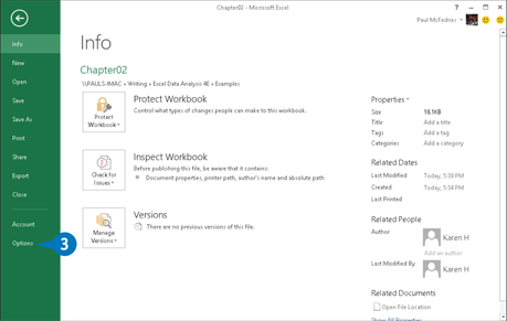
Click Options.

The Excel Options dialog box appears.

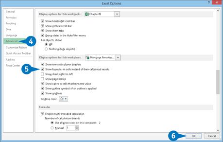
Click Advanced.

In the Display Options for This Worksheet section, click the Show Formulas in Cells Instead of Their Calculated Results check box ( changes to ).

Click OK.

A Excel displays the formulas instead of their results.

Note: You can also toggle the display between formulas and results by pressing Ctrl+`.

Use a Watch Window to Monitor a Cell Value

When you build a spreadsheet, it is often useful to monitor a cell’s value, particularly if that cell contains a formula. For example, if a cell calculates the average of a range of values, you might want to monitor the average as the data changes to see if it reaches a particular value.

Monitoring a cell value is not easy if the cell’s formula resides in a different worksheet or off-screen in the current worksheet. Rather than constantly navigating back and forth to check the cell value, you can use the Watch Window to monitor it. The Watch Window stays onscreen all the time, so no matter where you are within Excel, you can see the value of the cell.

Use a Watch Window to Monitor a Cell Value

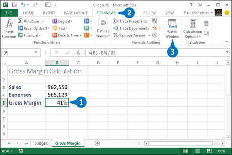
Select the value you want to watch.

Click the Formulas tab.

Click Watch Window.

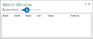
The Watch Window appears.

Click Add Watch.

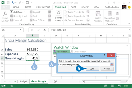
The Add Watch dialog box appears.

A The selected cell appears in the reference box.

B If the cell is incorrect, you can click the cell you want to monitor.

Click Add.

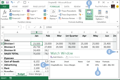
C Excel adds the cell to the Watch Window.

D The value of the cell appears here.

As you work with Excel, the Watch Window stays on top of the other windows so you can monitor the cell value.

E If the Watch Window gets in the way, you can hide it by either clicking the Close button (X) or clicking Watch Window in the Formula tab.

Step Through a Formula

Many Excel formulas can be quite complex, with functions nested inside other functions, multiple sets of parentheses, several different operators, multiple range references, and so on. These more involved formulas are much harder to troubleshoot because it is often unclear what part of the formula is causing the trouble.

You can use the Evaluate Formula command to help troubleshoot such formulas. This command enables you to step through the various parts of the formula to see the preliminary results returned by each part. By examining these interim results, you can often see where your formula goes awry. If you still have trouble pinpointing the error, see the Audit a Formula to Locate Errors section in this chapter.

Step Through a Formula

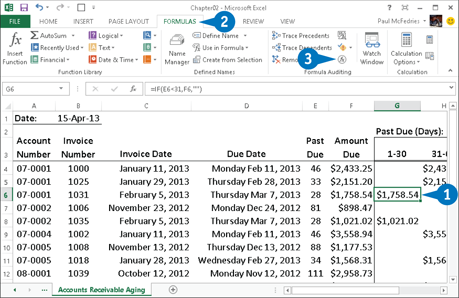
Select the cell that contains the formula you want to troubleshoot.

Click the Formulas tab.

Click Evaluate Formula.

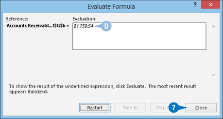
The Evaluate Formula dialog box appears.

A Excel underlines the first expression that it will evaluate.

Click Evaluate.

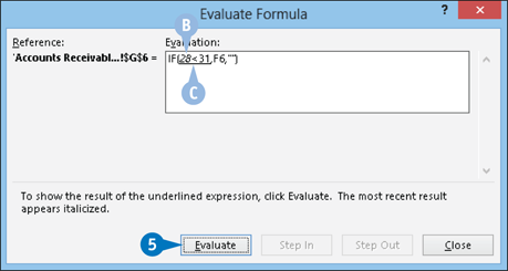
B Excel evaluates the underlined term and then displays the result in italics.

C Excel underlines the next expression that it will evaluate.

Click Evaluate.

Repeat step 5 to continue evaluating the formula’s expressions.

Note: Continue evaluating the formula until you find the error or you want to stop the evaluation.

D If you evaluate all the terms in the formula, Excel displays the final result.

Click Close.

Display Text Instead of Error Values

If Excel encounters an error when calculating a formula, it often displays an error value as the result. For example, if your formula divides by zero, Excel indicates the error by displaying the value #DIV/0. There may be times when you know the error is temporary or is otherwise unimportant. For example, if your worksheet is missing data, then a blank cell might be causing the #DIV/0 error. Rather than displaying an error value, you can use the IFERROR function to test for an error and display a more useful result in the cell:

IFERROR(value, value_if_error)

Here, value is the formula you are using, and value_if_error is the text you want Excel to display if the formula produces an error.

Display Text Instead of Error Values

Select the range that contains the formulas you want to edit.

Press F2.

A Excel opens the first cell for editing.

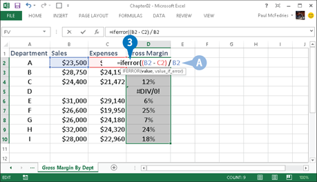
After the formula’s equals sign (=), type iferror(.

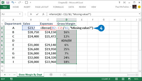
After the formula, type a comma followed by the text, in quotation marks, that you want Excel to display in place of any error, followed by a closing parenthesis.

Press Ctrl+Enter.

B Excel displays the formula result in cells where there is not an error.

C Excel displays the text message in cells that generate an error.

Check for Formula Errors in a Worksheet

If you use Microsoft Word, you are probably familiar with the wavy green lines that appear under words and phrases that the grammar checker has flagged as being incorrect. Excel has a similar feature: the formula error checker. It is similar to the grammar checker, in that it uses a set of rules to determine correctness, and it operates in the background to monitor your formulas. If it detects that something is amiss, it displays an error indicator — a green triangle — in the upper-left corner of the cell containing the formula. You can then use the associated smart tag to see a description of the error and to either fix or ignore the error.

Check for Formula Errors in a Worksheet

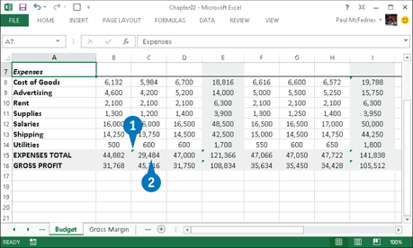
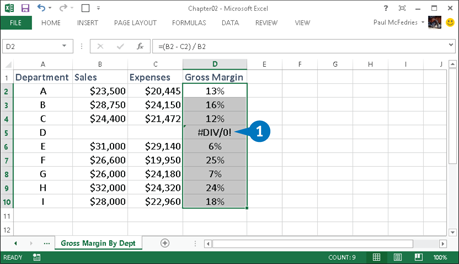
Examine your worksheet for a cell that displays the error indicator.

Click the cell.

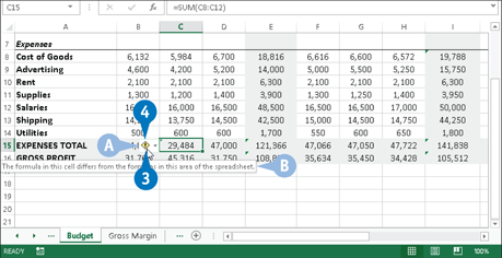
A The error smart tag appears.

Position the mouse pointer over the smart tag.

B Excel displays a description of the error.

Click the smart tag.

C Excel displays the smart tag options.

Click the command that fixes the formula.

Note: The name of the command depends on the error. You only see this command if Excel can fix the error.

D If the indicated error is not actually an error, you can just click Ignore Error.

E Excel adjusts the formula.

F Excel removes the error indicator from the cell.

Repeat steps 1 to 5 until you have checked all your worksheet formula errors.

Audit a Formula to Locate Errors

To determine which cell is causing an error in your formula, you can use the auditing features in Excel to visualize and trace a formula’s input values and error sources. Auditing operates by creating tracers — arrows that literally point out the cells involved in a formula. You can use tracers to find three kinds of cells. Precedents are cells that are directly or indirectly referenced in a formula. Dependents are cells that are directly or indirectly referenced by a formula in another cell. Errors are cells that contain an error value and are directly or indirectly referenced in a formula.

Audit a Formula to Locate Errors

Trace Precedents

Click the cell containing the formula whose precedents you want to trace.

Click the Formulas tab.

Click Trace Precedents.

A Excel adds a tracer arrow to each direct precedent.

Repeat step 3 until you have added tracer arrows for all the formula’s indirect precedents.

Trace Dependents

Click the cell containing the formula whose dependents you want to trace.

Click the Formulas tab.

Click Trace Dependents.

B Excel adds a tracer arrow to each direct dependent.

Repeat step 3 until you have added tracer arrows for all the formula’s indirect dependents.

Trace Errors

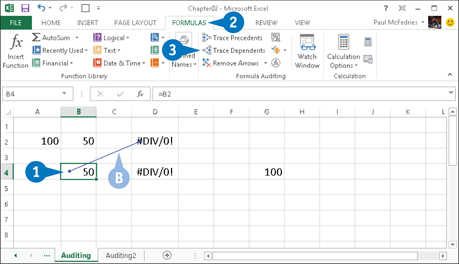
Click the cell containing the error you want to trace.

Click the Formulas tab.

Click Remove Arrows.

Note: You must first remove any existing arrows before you can trace an error.

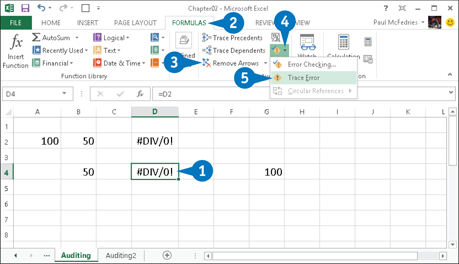
Click the Error Checking down arrow.

Click Trace Error.

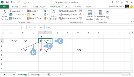
C Excel selects the cells that contain the original error.

D Excel displays tracer arrows showing the selected cells’ precedents and dependents.

E A red tracer arrow indicates an error.