Chapter 3

Enhancing Formulas with Functions

Understanding Excel Functions

A function is a predefined formula that accepts one or more inputs and then calculates a result. In Excel, a function is often called a worksheet function because you normally use it as part of a formula that you type in a worksheet cell. However, Excel enables you to use many of its worksheet functions in other parts of the program, such as VBA macros and the PivotTable formulas you create for calculated fields and items. This section introduces you to worksheet functions by showing you their advantages and structure and by examining a few other worksheet ideas that you should know.

Function Advantages

Functions are designed to take you beyond the basic arithmetic and comparison formulas. Functions do this in three ways:

• Functions make simple but cumbersome formulas easier to use. For example, suppose that you have a worksheet showing average house prices in various neighborhoods and you want to calculate the monthly mortgage payment for each price. Given a fixed monthly interest rate and a term in months, here is the general formula for calculating the monthly payment:

House Price * Interest Rate / (1 - (1 + Interest Rate) ^ -Term)

Fortunately, Excel offers an alternative to this intimidating formula — the PMT (payment) function:

PMT(Interest Rate, Term, House Price)

Not only is this simpler than the equivalent worksheet formula, but Excel also helps you to enter a formula correctly by displaying a pop-up banner that shows you the exact syntax to use for each function.

• Functions enable you to include complex mathematical expressions in your worksheets that otherwise are difficult or impossible to construct using simple arithmetic operators. For example, you can calculate a range’s average value using the AVERAGE function, but what if you prefer to know the median — the value that falls in the middle when all the values are sorted numerically — or the mode, which is the value that occurs most frequently? Either value can be time consuming to calculate by hand, but both are easy to calculate using the MEDIAN and MODE worksheet functions in Excel. Depending on your data analysis needs, you can also use functions to round formula results to a specified number of decimal places, calculate conditional sums and counts, and find square roots

• Functions enable you to include data in your applications that you could not access otherwise. For example, the powerful IF function enables you to test the value of a cell — for example, to see whether it contains a particular value — and then return one value or another, depending on the result. Similarly, the INFO function can tell you how much memory is available on your system, what operating system you are using, the version number of the operating system, the Excel version number, and more.

• Functions enable you to access other values in a worksheet depending on certain criteria, the result of another formula, and so on. These so-called lookup functions such as VLOOKUP and HLOOKUP can use a special range called a lookup table to seek a value in a specified lookup column that contains the values that you look up, and return a value from the data column that contains the data associated with each lookup value.

Function Structure

To use worksheet functions efficiently and to help you figure out how each function operates, you need to understand the structure of a typical function, particularly its name, and its arguments. Every worksheet function has the same basic structure of

NAME(Argument1, Argument2, ...)

Function Name

The NAME part identifies the function. In worksheet formulas, the function name always appears in uppercase letters: PMT, SUM, AVERAGE, and so on.

No matter how you type a function name, Excel always converts the name to all-uppercase letters. Therefore, when you type the name of a function that you want to use in a formula, you should always type the name using lowercase letters. This way, if you find that Excel does not convert the function name to uppercase characters, it means you misspelled the name, because Excel does not recognize it.

Arguments

The items that appear within the parentheses are the functions’ arguments. The arguments are the inputs that functions use to perform calculations. For example, the SUM function adds its arguments and the PMT function calculates the loan payment based on arguments that include the interest rate, term, and present value of the loan. Some functions do not require any arguments at all, but most require at least one argument, and some as many as nine or ten. If a function uses two or more arguments, be sure to separate each argument with a comma, and be sure to enter the arguments in the order specified by the function.

Function arguments fall into two categories: required and optional. A required argument is one that you must specify when you use the function, and it must appear within the parentheses in the specified position; if you omit a required argument, Excel generates an error. An optional argument is one that you are free to use or omit, depending on your needs. If you omit an optional argument, Excel uses the argument’s default value in the function. For example, the PMT function has an optional “future value” argument with which you can specify the value of the loan at the end of the term. The default future value is 0, so you need only specify this argument if your loan’s future value is something other than 0.

Excel uses two methods for differentiating between required and optional arguments. When you enter a function in a cell, the optional arguments are shown surrounded by square brackets: [ and ]. When you build a function using the Insert Function dialog box, or look up a function in the Excel Help system, required arguments are shown in bold text and optional arguments are shown in regular text.

If a function has multiple optional arguments, you may need to skip one or more of these arguments. If you do this, be sure to include the comma that would normally follow each missing argument. For example, here is the full PMT function syntax (the required arguments are shown in bold text):

PMT(rate, nper, pv, fv, type)

Here is an example PMT function that uses the type argument but not the fv argument:

PMT(0.05, 25, 100000, ,1)

Understanding Function Types

Excel comes with hundreds of worksheet functions, and they are divided into various categories or types. These function types include Text, Information, Lookup and Reference, Date and Time, and Database. Although you will often use these categories for Excel data analysis, there are four function types that you will most likely use in most of your analytical formulas: Math, Statistical, Financial, and Logical. This section introduces you to these four function types and lists the most popular and useful functions in each category. Note that for each function, the required arguments appear in bold type.

Mathematical Functions

You use the mathematical worksheet functions in Excel to manipulate numbers. The following table lists a few of the most useful mathematical functions.

Function	Description
CEILING(number,significance)	Rounds number up to the nearest integer
EVEN(number)	Rounds number up to the nearest even integer
FACT(number)	Returns the factorial of number
FLOOR(number,significance)	Rounds number down to the nearest multiple of significance
INT(number)	Rounds number down to the nearest integer
MOD(number,divisor)	Returns the remainder of number after dividing by divisor
ODD(number)	Rounds number up to the nearest odd integer
PI()	Returns the value Pi
PRODUCT(number1,number2,...)	Multiplies the specified numbers
RAND()	Returns a random number between 0 and 1
ROUND(number,digits)	Rounds number to a specified number of digits
ROUNDDOWN(number,digits)	Rounds number down, toward 0
ROUNDUP(number,digits)	Rounds number up, away from 0
SIGN(number)	Returns the sign of number (1 = positive; 0 = zero; –1 = negative)
SQRT(number)	Returns the square root of number
SUM(number1,number2,...)	Adds the arguments
TRUNC(number,digits)	Truncates number to an integer

Statistical Functions

Excel offers statistical functions that calculate a wide variety of highly technical statistical measures. The following table lists the worksheet functions that perform these basic statistical operations. For more information, see Chapter 5.

Function	Description
AVERAGE(number1,number2,...)	Returns the average of the arguments
COUNT(number1,number2,...)	Counts the numbers in the argument list
MAX(number1,number2,...)	Returns the maximum value of the arguments
MEDIAN(number1,number2,...)	Returns the median value of the arguments
MIN(number1,number2,...)	Returns the minimum value of the arguments
MODE(number1,number2,...)	Returns the most common value of the arguments
STDEV.P(number1,number2,...)	Returns the standard deviation based on an entire population
STDEV.S(number1,number2,...)	Returns the standard deviation based on a sample
Function	Description
VAR.P(number1,number2,...)	Returns the variance based on an entire population
VAR.S(number1,number2,...)	Returns the variance based on a sample

Financial Functions

The financial functions in Excel offer you powerful tools for calculating such things as the future value of an annuity and the periodic payment for a loan. The financial functions that you can use within your worksheets use the following arguments.

Argument	Description
rate	The fixed rate of interest over the term of the loan or investment
nper	The number of payments or deposit periods over the term of the loan or investment
pmt	The periodic payment or deposit
pv	The present value of the loan (the principal) or the initial deposit in an investment
fv	The future value of the loan or investment
type	The type of payment or deposit: 0 (the default) for end-of-period payments or deposits; 1 for beginning-of-period payments or deposits

The following table lists some worksheet functions that perform basic financial analysis. For examples, see Chapter 4.

Function	Description
FV(rate,nper,pmt,pv,type)	Returns the future value of an investment or loan
IPMT(rate,per,nper,pv,fv,type)	Returns the interest payment for a specified period of a loan
NPER(rate,pmt,pv,fv,type)	Returns the number of periods for an investment or loan
PMT(rate,nper,pv,fv,type)	Returns the periodic payment for a loan or investment
PPMT(rate,per,nper,pv,fv,type)	Returns the principal payment for a specified period of a loan
PV(rate,nper,pmt,fv,type)	Returns the present value of an investment
RATE(nper,pmt,pv,fv,type,guess)	Returns the periodic interest rate for a loan or investment

Logical Functions

The logical functions operate with the logical values TRUE and FALSE, which in your worksheet calculations are interpreted as 1 and 0, respectively. In most cases, the logical values used as arguments are expressions that use comparison operators such as equal to (=) and greater than (>). The following table lists the logical functions that you can use in your formulas.

Function	Description
AND(logical1,logical2,...)	Returns 1 if all the arguments are true; returns 0, otherwise
IF(logical_test,true_expr,false_expr)	Performs a logical test; returns true_expr if the result is 1 (true); returns false_expr if the result is 0 (false)
NOT(logical)	Reverses the logical value of the argument
OR(logical1,logical2,...)	Returns 1 if any argument is true; returns 0, otherwise

Add a Function to a Formula

To get the benefit of an Excel function, you need to use it within a formula. You can use a function as the only operand in the formula, or you can include the function as part of a larger formula. To make it easy to choose the function you need and to add the appropriate arguments, Excel offers the Insert Function feature. This dialog box enables you to display functions by category and then choose the function you want from a list. You then see the Function Arguments dialog box that enables you to easily see and fill in the arguments used by the function.

Add a Function to a Formula

Click in the cell in which you want to build the formula.

Type =.

Type any operands and operators you need before adding the function.

Click the Insert Function button.

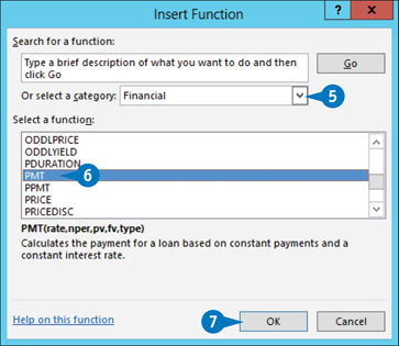
The Insert Function dialog box appears.

Click the down arrow and then select the category that contains the function you want to use from the drop-down list.

Click the function.

Click OK.

The Function Arguments dialog box appears.

Click inside an argument box.

Click the cell that contains the argument value.

You can also type the argument value.

Repeat steps 8 and 9 to fill as many arguments as you need.

A The function result appears below the edit boxes.

Click OK.

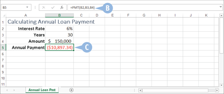
B Excel adds the function to the formula.

C Excel displays the formula result.

Note: In this example, the result appears in the parentheses to indicate a negative value. In loan calculations, money that you pay out is always a negative amount.

Note: If your formula requires any other operands and operators, press F2 and then type what you need to complete your formula.

Add a Row or Column of Numbers

You can quickly add worksheet numbers by building a formula that uses the Excel SUM function. When you use the SUM function in a formula, you can specify as the function’s arguments a series of individual cells. For example, SUM(A1, B2, C3) calculates the total of the values in cells A1, B2, and C3. However, you can also use the SUM function to specify just a single argument, which is a range reference to either a row or a column of numbers. For example, SUM(C3:C21) calculates the total of the values in all the cells in the range C3 to C21.

Add a Row or Column of Numbers

Click in the cell where you want the sum to appear.

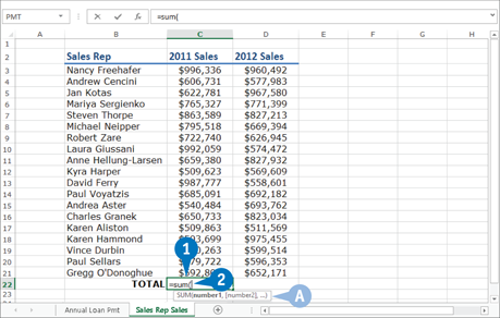
Type =sum(.

A When you begin a function, Excel displays a banner that shows you the function’s arguments.

Note: In the function banner, bold arguments are required, and arguments that appear in square brackets are optional.

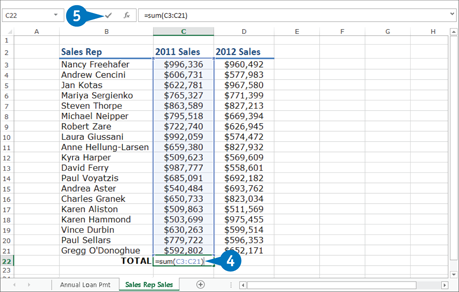
Click and drag the row or column of numbers that you want to add.

B Excel adds a reference for the range to the formula.

Type 20.

Click the Enter button or press Enter.

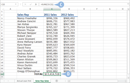
C Excel displays the formula.

D Excel displays the sum in the cell.

Build an AutoSum Formula

Creating formulas that sum one or more ranges is one of the simplest and most common data analysis tasks. In many cases, you can reduce the time it takes to build a worksheet as well as reduce the possibility of errors by using the Excel AutoSum feature. This tool adds a SUM function formula to a cell and automatically adds the function arguments based on the structure of the worksheet data. For example, if there is a column of numbers above the cell where you want the SUM function to appear, AutoSum automatically includes that column of numbers as the SUM function argument.

Build an AutoSum Formula

Click in the cell where you want the sum to appear.

Note: For AutoSum to work, the cell you select should be below or to the right of the range you want to sum.

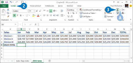
Click the Home tab.

Click the Sum button.

A If you want to use a function other than SUM, click the Sum down arrow and then click the operation that you want to use from the drop-down list, for example: Average, Count Numbers, Max, or Min.

B Excel adds a SUM function formula to the cell.

Note: You can also press Alt+= instead of clicking the Sum button.

C Excel guesses that the range above (or to the left of) the cell is the one you want to add.

If Excel guessed wrong, you can select the correct range manually.

Click the Enter button or press Enter.

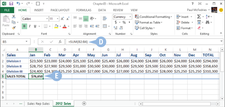
D Excel displays the formula.

E Excel displays the sum in the cell.

Round a Number

When you need to round numbers, Excel offers the ROUND function, which rounds a value to the number of digits you specify. It takes two arguments: Number, the value you want to round, and Num_digits, the number of digits to which you want to round your number. If Num_digits is 1 or higher, Excel rounds to the number of decimal places that you specify. If Num_digits is 0, Excel rounds to the nearest integer. If Num_digits is –1 or lower, Excel rounds to the number of digits you specify that are to the left of the decimal point. For example, the function =ROUND(1234.5678,2) rounds to 1234.57, the function =ROUND(1234.5678,0) rounds to 1235, and the function =ROUND(1234.5678, –2) rounds to 1200.

Round a Number

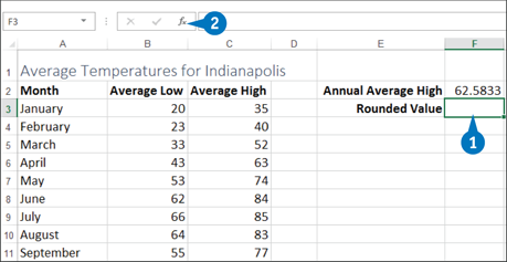
Click the cell where you want the result to appear.

Click the Insert Function button.

The Insert Function dialog box appears.

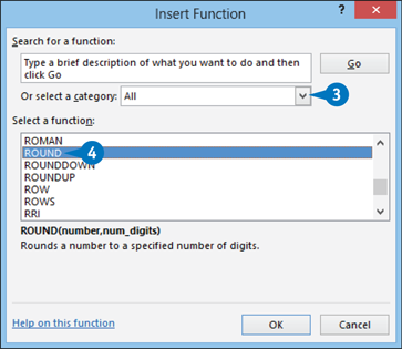
Click the select a category down arrow and then select All from the drop-down list to list all the functions.

Double-click ROUND.

The Function Arguments dialog box appears.

Enter the cell address of the number you want to round.

Alternatively, if the number is not in a cell, you can type the number into the Number field.

Type the number of decimal places to which you want to round.

Click OK.

A Excel rounds the number.

Create a Conditional Formula

A conditional formula uses the IF function to return a value based on whether a specified condition is true. The IF function takes three arguments: logical_test, value_if_true, and value_if_false. The logical_test argument is the condition being evaluated. It is a logical expression — that is, one that uses a comparison operator, such as greater than (>), less than or equal to (<=), or equal to (=) — that returns either the value TRUE or the value FALSE. The value_if_true argument is the result that the IF function returns if the logical_test argument is TRUE; the value_if_false argument is the result that the IF function returns if the logical_test argument is FALSE.

Create a Conditional Formula

Double-click the cell where you want your conditional formula to appear.

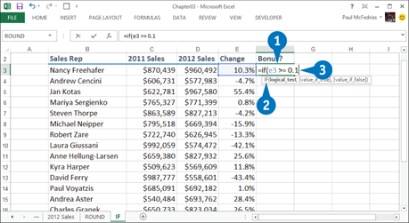
Type =if(.

Type the logical expression you want the IF function to evaluate.

Type a comma (,) followed by the value you want the IF function to return if the logical expression evaluates to TRUE.

Note: If the value is text, surround it with double quotation marks.

Type a comma (,) followed by the value you want the IF function to return if the logical expression evaluates to FALSE.

Note: If the value is text, surround it with double quotation marks.

Type a closing parenthesis: 20.

Click the Enter button or press Enter.

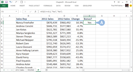
A Excel evaluates the logical expression and then displays the result in the cell.

Calculate a Conditional Sum

In your data analysis, you might need to sum the values in a range, but only those values that satisfy some condition. You can do this by using the SUMIF function, an amalgam of SUM and IF, which sums only those cells in a range that meet the condition you specify. SUMIF takes up to three arguments: range, which is the range of cells you want to use to test the condition; criteria, which is a text string that determines which cells in range to sum; and the optional sum_range, which is the range from which you want the sum values to be taken. Excel sums only those cells in sum_range that correspond to the cells in range and meet the criteria.

Calculate a Conditional Sum

In the cell where you want the result to appear, type =sumif(.

Type the range argument.

Type a comma (,) and then the criteria argument.

Note: Enclose the criteria argument in double quotation marks.

If required, type a comma (,) and then the sum_range argument.

Note: If you omit sum_range, Excel uses range for the sum.

Type 20.

Click the Enter button or press Enter.

A Excel displays the conditional sum in the cell.

Note: You can use the question mark (?) and asterisk (*) wildcards when creating your condition. A ? matches a single character, while an * matches multiple characters.

Calculate a Conditional Count

When analyzing data, you might need to count the items in a range, a task normally handled by the COUNT function. However, in some cases you might need to count only those values that meet a condition. You can do this by using the COUNTIF function, which combines the COUNT and IF functions. COUNTIF counts only those cells in a range that meet the condition you specify. COUNTIF takes two arguments: range, which is the range of cells you want to use to test the condition; and criteria, which is a text string that determines which cells in range to count.

Calculate a Conditional Count

In the cell where you want the result to appear, type =countif(.

Type the range argument.

Type a comma (,) and then the criteria argument.

Note: Enclose the criteria argument in double quotation marks.

Type 20.

Click the Enter button or press Enter.

A Excel displays the conditional count in the cell.

Note: You can use the question mark (?) and asterisk (*) wildcards when creating your condition. A ? matches a single character, while an * matches multiple characters.

Find the Square Root

You can use the SQRT function to find a number’s square root. However, Excel can only calculate the square roots of positive numbers. If a negative number is the argument, as in SQRT(–9), Excel returns the error #NUM. To calculate the positive square root of a negative number, you can use ABS to first calculate the number’s absolute value. The following formula returns 3: =SQRT(ABS(–9)). To find the power of any number, such as 2 to the fifth power, you can use the POWER function. This function takes two arguments: the number you want to raise to a power and the power to which you want to raise it. The formula =POWER(2, 5) raises the 2 to the fifth power, yielding 32.

Find the Square Root

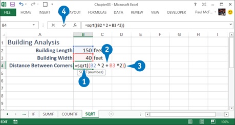
In the cell where you want the result to appear, type =sqrt(.

Type or select the value of which you want to find the square root.

Type 20.

Click the Enter button or press Enter.

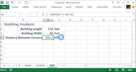
A Excel displays the square root in the cell.

Retrieve a Column or Row Number

When you use functions such as VLOOKUP or INDEX, you enter a column number, a row number, or both. Entering an actual number means that number will not change when you copy the formula to another cell. If you want the number to change in the same way that relative cell addresses change, you can use the COLUMN function or the ROW function. These functions take one optional argument, reference, which is the cell or range for which you want to retrieve the row or column number. If you omit this argument, Excel returns the column or row number of the current cell. If you enter a range, Excel returns the column or row number of the range’s upper-left corner cell.

Retrieve a Column or Row Number

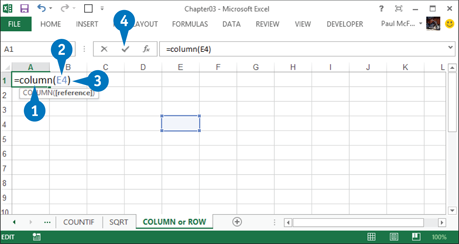
In the cell where you want the result to appear, type =column( or =row(.

If needed, type or select the cell or range for which you want to retrieve the column or row number.

Type 20.

Click the Enter button or press Enter.

A Excel displays the column or row number in the cell.

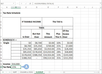
Look Up a Value

Use Excel’s lookup functions to look up a value within a range and return a corresponding item from that range. For example, you can look up an income value in a tax table and return the corresponding tax rate. To look up a value within a column, use VLOOKUP; to look up a value within a row, use HLOOKUP. These functions have three required arguments: lookup_value specifies the value you want to look up; table_array is the range of values; and col_index_num (or row_index_num for HLOOKUP) is the column (or row) number within table_array that contains the value to retrieve. An optional fourth argument is range_lookup: if you omit it, the function looks for the closest match; if you set it to FALSE, the function looks for an exact match.

Look Up a Value

In the cell where you want the retrieved value to appear, type =vlookup( or =hlookup(.

Type or select the value you want to look up.

Type a comma (,) followed by the address of the lookup range.

Note: Make sure the first column of the selected range is the column you want to use for the lookup.

Type a comma (,) followed by the column (if you are using VLOOKUP) or row (if you are using HLOOKUP) number that contains the value you want to retrieve.

Type a closing parenthesis, 20.

Click the Enter button or press Enter.

A Excel evaluates the logical expression and then displays the result in the cell.

Determine the Location of a Value

The MATCH function looks through a row or column for a value. If it finds a match, it returns the relative position of the match in the row or column. MATCH has three arguments: lookup_value is the value you want to find; lookup_array is the range you want to search; and the optional match_type specifies how to match values. If you omit match_type or enter 0, Excel finds the largest value less than or equal to lookup_value, and lookup_array must be in ascending order. If you enter –1, Excel returns the smallest value greater than or equal to lookup_value, and lookup_array must be in descending order. If you enter 0, Excel returns the first value that exactly matches lookup_value, and lookup_array can be in any order.

Determine the Location of a Value

In the cell where you want the result to appear, type =match(.

Type the value you want to locate or enter its address.

Type the address of the column or row you want to search.

Enter the match_type value.

Type 20.

Click the Enter button or press Enter.

A If Excel finds a match, it displays the relative position of the match within the row or column.

Note: If you see the #NA! error, it means Excel did not find a match.

Return a Cell Value with INDEX

If a particular value exists within a range, you can say that value resides at the intersection of a row and column number within the range. To retrieve that value, you can use the INDEX function. INDEX takes four arguments: reference specifies one or more ranges; row_num is the row number in reference from which to return a value; the optional column_num is the column number in reference from which to return a value; and area_num is the range you want to use if reference consists of multiple ranges, where the first range is 1, the second is 2, and so on. In most uses of INDEX, you use MATCH, described in the previous section, to return the row_num or column_num argument.

Return a Cell Value with INDEX

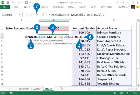
In the cell where you want the result to appear, type =index(.

Type the address of the range you want to search.

Type the row number of the value you want to return.

Type the column number of the value you want to return.

Note: You can omit column_num if the range you are using is a single column.

If you entered multiple ranges in step 2, type the range number you want to use (not shown).

Type 20.

Click the Enter button or press Enter.

A If Excel locates the cell, it displays the cell’s value.

Note: If you see the #NA! error, it means Excel did not locate the cell.

Perform Date and Time Calculations

In your Excel data analysis work, you will often have to perform date and time calculations. You can find, for example, the number of days that have elapsed between the start of a project and the end of a project or the number of hours worked from the start of the workday to the end of the workday.

Serial Numbers

Excel bases every date and time on a serial number that it can use to add and subtract. Excel calculates a date’s serial number as the number of days after December 31, 1899, and represents each date with a whole number. Excel calculates a time’s serial number as a value between 0 and 1, where midnight is 0, 6 a.m. is 0.25, noon is 0.5, and so on. A combined date and time serial number consists of the date to the left of the decimal and a time to the right. For example, August 23, 2013 6:00 p.m. has the serial number is 41509.75.

Date Calculations

Excel enables you to perform date calculations by returning a date serial number, returning parts of a date, such as the year or month, and determining the difference between two dates. This enables you to include sophisticated date calculations in your data analysis worksheets.

Return a Date

If you need a date for an expression operand or a function argument, you can always enter it by hand if you have a specific date in mind. Much of the time, however, you need more flexibility, such as always entering the current date or building a date from day, month, and year components. Excel offers three functions that can help: TODAY, DATE, and DATEVALUE. Use the TODAY function when you need to use the current date in a formula, function, or expression. Note that TODAY does not take any arguments. Use the DATE function to build a date from three separate values: the year, month, and day. DATE takes three arguments: year, which is the year component of the date (a number between 1900 and 9999); month, which is the month component of the date; and day, which is the day component of the date. For example, DATE(2013, 12, 25) returns the serial number of Christmas Day in 2013. Use DATEVALUE if you have a date value in string form and you want to convert it to a date serial number. DATEVALUE takes a single argument called date_text that is the string containing the date. For example, DATEVALUE(“August 23, 2013”) returns the date serial number for the string August 23, 2013.

Return Parts of a Date

The three components of a date — year, month, and day — can also be extracted individually from a given date. This might not seem very interesting at first, but many useful techniques actually arise out of working with a date’s component parts. A date’s components are extracted using the Excel YEAR, MONTH, and DAY functions, each of which takes a single argument called serial_number, which is the date you want to work with.

Calculate the Difference between Two Dates

Subtracting one date or time from another involves subtracting one serial number from another. For example, the serial number for August 14, 2013 is 41500 and the serial number for October 13, 2013 is 41560. To obtain the number of days between these two dates, subtract the later date from the earlier one. In this case, Excel performs the following calculation: = 41560 – 41500, which equal 60. However, when performing a date calculation, you do not need to display the serial number because Excel handles the conversion automatically.

Time Calculations

Excel enables you to perform time calculations by returning a time serial number; returning parts of a time, such as the hour or minute; and determining the difference between two times. These techniques enable you to include useful and sophisticated time calculations in your data analysis models.

Return a Time

The most straightforward way to work with times as operands or function arguments is to type the time values manually. Usually, however, your data analysis requires a more flexible approach, such as always using the current time or building a time using separate hour, minute, and second components. Excel offers three functions that can help: NOW, TIME, and TIMEVALUE. Use the NOW function when you need to use the current time in a formula, function, or expression. Note that NOW does not take any arguments. Use the TIME function to build a date from three separate values: the hour, minute, and second. TIME takes three arguments: hour, which is the hour component of the time (a number between 0 and 23); minute, which is the minute component of the time (between 0 and 59); and second, which is the second component of the time (between 0 and 59). For example, TIME(13, 30, 15) returns the serial number of the time 1:30:15 p.m. Use TIMEVALUE if you have a time value in string form and you want to convert it to a time serial number. TIMEVALUE takes a single argument called time_text that is the string containing the time. For example, TIMEVALUE(“4:45:00 PM”) returns the time serial number for the string 4:45:00 PM.

Return Parts of a Time

If you require them for your formula, you can extract the three components of a time: hour, minute, and second. A time’s components are extracted using the Excel HOUR, MINUTE, and SECOND functions, each of which takes a single argument called serial_number, which is the time you want to work with.

Calculate the Difference between Two Times

As with dates, you determine the difference between two time values by subtracting the later time from the earlier one. For example, if the later time is 6:00 p.m. and the earlier time is 9:00 a.m., Excel calculates the difference by using the serial numbers for the two times, which in this case is =0.75 - 0.375. The result is 0.375, which means the difference is 9 hours. When calculating the difference between two times, you want to know the hours and minutes that have elapsed, so you need to format your results as hours and minutes. Click the Home tab and then click the dialog box launcher in the Number group to open the Format Cells dialog box. Click the Number tab, click Time, click the format type 13:30, and then click OK. Also, when subtracting times that cross midnight, such as 11:00 p.m. to 2:00 a.m., you need to use the MOD function, which returns the remainder after dividing by a specified value. Here is the general formula to use:

=MOD
(later time – earlier time, 1)