
Chapter 1
Building Formulas for Data Analysis
Introducing Data Analysis
Data analysis is the application of tools and techniques to organize, study, reach conclusions, and sometimes make predictions about a specific collection of information. A sales manager might use data analysis to study the sales history of a product, determine the overall trend, and produce a forecast of future sales. A scientist might use data analysis to study experimental findings and determine the statistical significance of the results. A family might use data analysis to find the maximum mortgage that they can afford, or to determine how much they need to put aside each month to finance their retirement or their children’s education.
Manipulate Raw Data
The point of data analysis is to understand information on some deeper, more meaningful level. By definition, raw data is a mere collection of facts that by themselves tell you little or nothing of any importance. To gain some understanding of the data, you must manipulate it in some meaningful way. This can be something as simple as finding the sum or average of a column of numbers or as complex as employing a full-scale regression analysis to determine the underlying trend of a range of values. Both are examples of data analysis, and Excel offers a number of tools, from the straightforward to the sophisticated, to meet even the most demanding needs.
Data
The “data” part of data analysis is a collection of numbers, dates, and text that represents the raw information you have to work with. In Excel, this data resides inside a worksheet and you get it there in one of two ways: you enter it by hand or you import it from an external source. You can then either leave the data as a regular range, or convert it into a table for easier data manipulation.
Data Entry
In many data analysis situations, you must enter the required data into the worksheet manually. For example, if you want to determine a potential monthly mortgage payment, you must first enter values such as the current interest rate, the principal, and the term. Manual data entry is suitable for small projects only, because entering hundreds or even thousands of values is time- consuming and can lead to errors.
Imported Data
Most data analysis projects involve large amounts of data, and the fastest and most accurate way to get that data onto a worksheet is to import it from a non-Excel data source. In the simplest scenario, you can copy the data from a text file, a Word table, or an Access datasheet and then paste it into a worksheet. However, most business and scientific data is stored in large databases, and Excel offers tools to import the data you need into your worksheet. See Chapter 14 for more about these tools.
Table
After you have your data in the worksheet, you can leave it as a regular range and still apply many data analysis techniques to the data. However, if you convert the range into a table, Excel treats the data as a simple flat-file database and enables you to apply a number of database-specific analysis techniques to the table. To learn how to do this, see Chapter 6.
Data Models
In many cases, you perform data analysis on worksheet values by organizing those values into a data model, a collection of cells designed as a worksheet version of some real-world concept or scenario. The model includes not only the raw data, but also one or more cells that represent some analysis of the data.
Formulas
A formula is a set of symbols and values that perform some kind of calculation and produce a result. All Excel formulas have the same general structure: an equal sign (=) followed by one or more operands separated by one or more operators. Operands can be a value, a cell reference, a range, a range name, or a function name. Operators are the symbols that combine the operands in some way, such as the plus sign (+) and the multiplication sign (*). For example, the formula =A1+A2 adds the values in cells A1 and A2.
Functions
A function is a predefined formula that is built in to Excel. Each function takes one or more inputs called arguments, such as numbers or cell references, and then returns a result. Excel offers hundreds of functions and you can use them to compute averages, determine the future value of an investment, and much more.
What-If Analysis
One of the most common data analysis techniques is what-if analysis, where you set up worksheet models to analyze hypothetical situations. The what-if part comes from the fact that these situations usually come in the form of a question: “What happens to the monthly payment if the interest rate goes up by 2 percent?” Excel offers four what-if analysis tools: data tables, Goal Seek, Solver, and scenarios.
A data table is a range of cells where one column consists of a series of values, called input cells. You can then apply each of those inputs to a single formula, and Excel displays the results for each case. For example, you can use a data table to apply a series of interest rate values to a formula that calculates the monthly payment for a loan or mortgage.
Goal Seek
You use the Goal Seek tool in Excel when you want to manipulate one formula component, called the changing cell, in such a way that the formula produces a specific result. For example, in a break-even analysis, you can use Goal Seek to determine the number of units of a product that you must sell for the profit to be 0.
Solver
You use the Solver tool in Excel when you want to manipulate multiple formula components, called the changing cells, in such a way that the formula produces the optimal result. For example, you can use Solver to tackle the so-called transportation problem, where the goal is to minimize the cost of shipping goods from several product plants to various warehouses around the country.
Scenarios
A scenario is a collection of input values that you plug into formulas within a model to produce a result. The idea is that you make up scenarios for various situations — for example, best-case, worst-case, and so on — and the Excel Scenario Manager saves each one. Later you can apply any of the saved scenarios, and Excel automatically applies all the input values to the model.
Introducing Formulas
A formula is a set of symbols and values that perform some kind of calculation and produce a result. All Excel formulas have the same general structure: an equal sign (=) followed by one or more operands and operators. The equal sign tells Excel to interpret everything that follows in the cell as a formula. For example, if you type =5+8 into a cell, Excel interprets the 5+8 text as a formula, and displays the result (13) in the cell.
To build accurate and useful formulas, you need to know the components of a formula, including operands and operators. You also need to understand the importance of precedence when building a formula.
Operands
Operands are the values that the formula uses as the raw material for the calculation. In a formula, the operands can be constants, cell or range references, range names, or worksheet functions.
Cell and Range References
The most common type of operand that you can use in a formula is a reference to a worksheet location. This makes intuitive sense because data analysis typically involves working with one or more values on a worksheet, so your formulas need some way to incorporate those worksheet values. In the simplest case, your formula can refer to the address of a single cell. For example, the following formula returns a result that adds 5 to the value in cell A1:
=A1 + 5
Your formulas can also work with ranges, in which case you include the range coordinates in your calculation. For example, the following formula uses the Excel SUM function to return the total of the values in the range B1:B5):
=SUM(B1:B5)
Range Names
Range names are labels applied to a single cell or to a range of cells. You can use a defined name in place of the range coordinates. In particular, to include the range in a formula, you use the name instead of selecting the range or typing its coordinates. Range names also make your formulas intuitive and easy to read. For example, assigning the name BeverageSales to a range such as F1:F10 immediately clarifies the purpose of a formula such as the following:
=SUM(BeverageSales)
Range names also increase the accuracy of your formulas because you do not have to specify range coordinates.
Constants
A constant is a fixed value that you insert into a formula and use as is. For example, suppose you want a calculated item to return a result that is 10 percent greater than the value of the Beverage_Total item. In that case, you create a formula that multiplies the Beverage_Total item by the constant 110 percent, as shown here:
=Beverage_Total * 110%
In Excel formulas, the constant values are usually numbers, although when using comparison formulas you may occasionally use a string (text surrounded by double quotation marks, such as “January”) as a constant.
Worksheet Functions
You can use any of the built-in worksheet functions in Excel as operands in a formula. For example, you can use the AVERAGE function to compute the average of two or more items, or you can use logic functions such as IF and OR to create complex formulas that make decisions. See Chapter 3 for more details.
Operators
It is possible to use only an operand in a formula. For example, if you reference just a cell address after the opening equal sign (=), then the value returned by the formula is identical to the value in the referenced cell.
A formula that is equal to an existing cell is not particularly useful in data analysis. To create formulas that perform more interesting calculations, you need to include one or more operators. The operators are the symbols that the formula uses to perform the calculation.
In an Excel formula that contains two or more operands, each operand is separated by an operator, which combines the operands in some way, usually mathematically. Example operators include the plus sign (+) and the multiplication sign (*). For example, the formula =B1+B2 adds the values in cells B1 and B2. See the next section, Understanding Formula Types, for a complete list of the available operators.
Operator Precedence
Most of your formulas include multiple operands and operators. In many cases, the order in which Excel performs the calculations is crucial. For example, consider the following formula:
=3 + 5 ^ 2
If you calculate from left to right, the answer you get is 64 (3 + 5 equal 8, and 8 ^ 2 equal 64). However, if you perform the exponentiation first and then the addition, the result is 28 (5 ^ 2 equal 25, and 3 + 25 equal 28). Therefore, a single formula can produce multiple answers, depending on the order in which you perform the calculations.
To control this problem, Excel evaluates a formula according to a predefined order of precedence. You can also control the order of precedence yourself using parentheses; see the Tip in the section, Build a Formula, later in this chapter. This order of precedence enables Excel to calculate a formula unambiguously by determining which part of the formula it calculates first, which part second, and so on. The formula operators determine the order of precedence, as shown in the following table:
|
Symbol |
Operator |
Order of Precedence |
|
( ) |
Parentheses |
1st |
|
: (space) , |
Reference |
2nd |
|
– |
Negation |
3rd |
|
% |
Percentage |
4th |
|
^ |
Exponentiation |
5th |
|
* and / |
Multiplication and division |
6th |
|
+ and – |
Addition and subtraction |
7th |
|
& |
Concatenation |
8th |
|
= < <= > >= <> |
Comparison |
9th |
Understanding Formula Types
Worksheet formulas fall into four distinct types: arithmetic formulas for computing numeric results; comparison formulas for comparing one value with another; text formulas for combining two or more text strings; and reference formulas that combine two cell references or ranges to create a single joint reference.
Because you usually deal with numeric values within a formula, the operators you use determine the type of formula. For example, arithmetic formulas use arithmetic operators and comparison formulas use comparison operators. This section shows you the operators that define all four formula types.
Arithmetic Formulas
An arithmetic formula combines numeric operands with mathematical operators to perform a calculation. Numeric operands are numeric constants, functions that return numeric results, and cells, ranges, or range names that contain numeric values. Because data analysis models primarily deal with numeric data, arithmetic formulas are by far the most common formulas used in analysis calculations.
The following table lists the seven arithmetic operators that you can use to construct arithmetic formulas. Most of these operators are straightforward, but the exponentiation operator might require further explanation. The formula =x ^ y means that the value x is raised to the power y. For example, the formula =3 ^ 2 produces the result 9 (that is, 3 * 3 = 9). Similarly, the formula =2 ^ 4 produces 16 (that is, 2 * 2 * 2 * 2 = 16).

Comparison Formulas
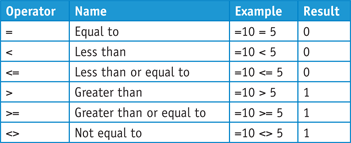
A comparison formula, also called a relational formula, combines numeric operands with special operators to compare one operand with another. Numeric operands are numeric constants, functions that return numeric results, and cells, ranges, or range names that contain numeric values. A comparison formula always returns a logical result. This means that if the comparison is true, then the formula returns the value 1, which is equivalent to the logical value TRUE; if the comparison is false, then the formula returns the value 0, which is equivalent to the logical value FALSE.
The following table lists the six operators that you can use to construct comparison formulas:
Text Formulas
You use text formulas not to derive a result, but to combine two or more text strings, a process known as concatenation. There is only one text concatenation operator — the ampersand (&). You use the ampersand to join values together to produce one continuous text value. For example, if the text “John” is in cell A1 and the text “Smith” is in cell B1, the formula = A1 & " " & B1 returns the concatenated string “John Smith” (in this formula, note that a space surrounded by double quotation marks returns a space). Your text formulas can also include text constants, which are text values surrounded by double quotation marks. For example, the formula ="John" & B1, returns “John Smith”, if "Smith" is in cell B1.
Reference Formulas
You use reference formulas to specify the range of cells you want to use in your formula. There are three reference operators: the colon (:), the comma (,), and the space. Excel refers to them as the range operator, the union operator, and the intersection operator, respectively. The colon references every cell included in and between the referenced cells. For example, A1:C3 includes cells A1, A2, A3, B1, B2, B3, C1, C2, and C3. The comma enables you to reference the union of two or more cells or ranges. For example, A1, B2:C3 references cells A1, B2, B3, C2, and C3. The intersection operator references all the cells that range operators have in common. For example, the reference B1:C3 C1:D3 references cells C1 to C3. You can use more than one reference operator in a single formula.
|
Operator |
Name |
Description |
|
: (colon) |
Range |
Produces a range from two cell references (for example, A1:C5) |
|
, (comma) |
Union |
Produces a range that is the union of two ranges (for example, A1:C5,B2:E8) |
|
(space) |
Intersection |
Produces a range that is the intersection of two ranges (for example, A1:C5 B2:E8 references the intersecting range B2:C5) |
Build a Formula
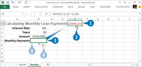
You can add a formula to a worksheet cell using a technique similar to adding data to a cell. To ensure that Excel treats the text as a formula, be sure to begin with an equal sign (=) and then type your operands and operators.
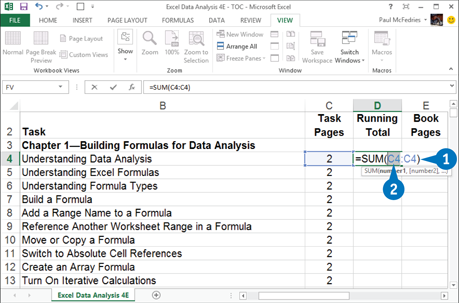
When you add a formula to a cell, Excel displays the formula result in the cell, not the actual formula. For example, if you add the formula =C3+C4 to a cell, that cell displays the sum of the values in cells C3 and C4. To see the formula, you can click the cell and examine the Formula bar.
Build a Formula
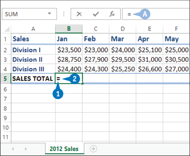
![]() Click in the cell in which you want to build the formula.
Click in the cell in which you want to build the formula.
![]() Type =.
Type =.
A Your typing also appears in the Formula bar.
Note: You can also type the formula into the Formula bar.

![]() Type or click an operand. For example, to reference a cell in your formula, click in the cell.
Type or click an operand. For example, to reference a cell in your formula, click in the cell.
B Excel inserts the address of the clicked cell into the formula.

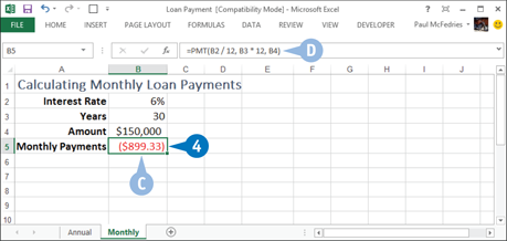
![]() Type an operator.
Type an operator.
![]() Repeat steps 3 and 4 to add other operands and operators to your formula.
Repeat steps 3 and 4 to add other operands and operators to your formula.
![]() Click the Enter button or press Enter.
Click the Enter button or press Enter.
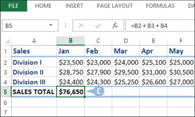
C Excel displays the formula result in the cell.
Add a Range Name to a Formula
You can make your formulas easier to build, more accurate, and easier to read by using range names as operands instead of cell and range addresses. For example, the formula =SUM(B2:B10) is difficult to decipher on its own, particularly if you cannot see the range B2:B10 to examine its values. However, if you use the formula =SUM(Expenses) instead, it becomes immediately obvious what the formula is meant to do. The easiest way to define a range name is to select the range and then type the name in the Name box, which appears on the far-left side of the Excel Formula bar.
Add a Range Name to a Formula
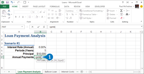
![]() Click in the cell in which you want to build the formula, type =, and then type any operands and operators you need before adding the range name.
Click in the cell in which you want to build the formula, type =, and then type any operands and operators you need before adding the range name.
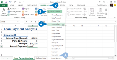
![]() Click the Formulas tab.
Click the Formulas tab.
![]() Click Use in Formula.
Click Use in Formula.
A Excel displays a list of the range names in the current workbook.
![]() Click the range name you want to use.
Click the range name you want to use.

B Excel inserts the range name into the formula.
![]() Type any operands and operators you need to complete your formula.
Type any operands and operators you need to complete your formula.
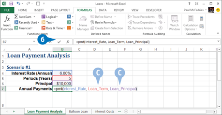
C If you need to insert other range names into your formula, repeat steps 2 to 5 for each name.
![]() Click the Enter button or press Enter.
Click the Enter button or press Enter.
Excel calculates the formula result.
Reference Another Worksheet Range in a Formula
You can enhance your data analysis and add flexibility to your formulas by adding references to ranges that reside in other worksheets. This enables you to take advantage of work that you or another person has done in other worksheets, so you do not have to waste time repeating that work in the current worksheet.
Referencing a range in another worksheet also gives you the advantage of having automatically updated information. For example, if the data in the other worksheet range changes, Excel automatically updates your formula to include the changed data. This saves you from constantly having to monitor the value in the other worksheet.
Reference Another Worksheet Range in a Formula

![]() Click in the cell in which you want to build the formula, type =, and then type any operands and operators you need before adding the range reference.
Click in the cell in which you want to build the formula, type =, and then type any operands and operators you need before adding the range reference.
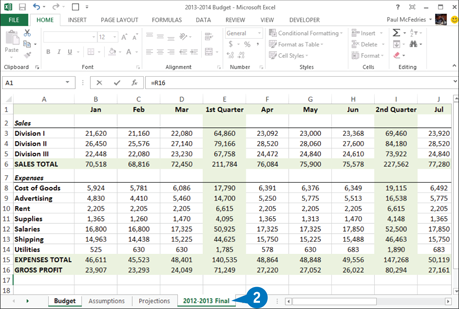
![]() Press Ctrl+Page Down until the worksheet you want to use appears.
Press Ctrl+Page Down until the worksheet you want to use appears.
![]() Select the range you want to use.
Select the range you want to use.
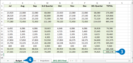
![]() Press Ctrl+Page Up until you return to the original worksheet.
Press Ctrl+Page Up until you return to the original worksheet.

A A reference to the range on the other worksheet appears in your formula.
![]() Type any operands and operators you need to complete your formula.
Type any operands and operators you need to complete your formula.
![]() Click the Enter button or press Enter.
Click the Enter button or press Enter.
Excel calculates the formula result.
Move or Copy a Formula
When you add a formula to a worksheet, the location of that formula is not fixed. You can restructure or reorganize a worksheet by moving an existing formula to a different part of the worksheet. When you move a formula, Excel preserves the formula’s range references.
Excel also enables you to make a copy of a formula, which is a useful technique if you require a duplicate of the formula elsewhere or if you require a formula that is similar to an existing formula. When you copy a formula, Excel adjusts the range references to the new location.
Move or Copy a Formula
Move a Formula
![]() Click the cell that contains the formula you want to move.
Click the cell that contains the formula you want to move.
![]() Position the mouse pointer over any outside border of the cell (
Position the mouse pointer over any outside border of the cell (![]() changes to
changes to ![]() ).
).
![]() Click and drag the cell to the new location (
Click and drag the cell to the new location (![]() changes to
changes to ![]() ).
).
A Excel displays an outline of the cell.
B Excel displays the address of the new location.
![]() Release the mouse button.
Release the mouse button.
C Excel moves the formula to the new location.
D Excel does not change the formula’s range references.
Copy a Formula
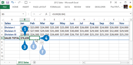
![]() Click the cell that contains the formula you want to copy.
Click the cell that contains the formula you want to copy.
![]() Press and hold the Ctrl key.
Press and hold the Ctrl key.
![]() Position the mouse pointer over any outside border of the cell (
Position the mouse pointer over any outside border of the cell (![]() changes to
changes to ![]() ).
).
![]() Click and drag the cell to the location where you want the copy to appear.
Click and drag the cell to the location where you want the copy to appear.
E Excel displays an outline of the cell.
F Excel displays the address of the new location.
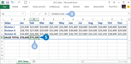
![]() Release the mouse button.
Release the mouse button.
![]() Release the Ctrl key.
Release the Ctrl key.
G Excel creates a copy of the formula in the new location.
H Excel adjusts the range references.
Note: You can make multiple copies by dragging the bottom-right corner of the cell. Excel fills the adjacent cells with copies of the formula. See the following section, Switch to Absolute Cell References, for an example.
Switch to Absolute Cell References
When you reference a cell in a formula, Excel treats it as a relative cell reference, which means it sees the reference as being relative to the formula’s cell. For example, if the formula is in cell B5 and it references cell A1, Excel effectively treats A1 as the cell four rows up and one column to the left. If you copy the formula to cell D10, then the cell four rows up and one column to the left is now cell C6, so in the copied formula Excel changes A1 to C6.
To prevent that reference from changing, you must use the absolute cell reference format: $A$1. In this case, the copied formula in cell D10 also refers to $A$1.
Switch to Absolute Cell References
![]() Double-click the cell that contains the formula you want to edit.
Double-click the cell that contains the formula you want to edit.
![]() Select the cell reference you want to change.
Select the cell reference you want to change.
![]() Press F4.
Press F4.

A Excel switches the address to an absolute cell reference.
![]() Repeat steps 2 and 3 to switch any other cell addresses that you require in the absolute reference format.
Repeat steps 2 and 3 to switch any other cell addresses that you require in the absolute reference format.
![]() Click the Enter button or press Enter.
Click the Enter button or press Enter.
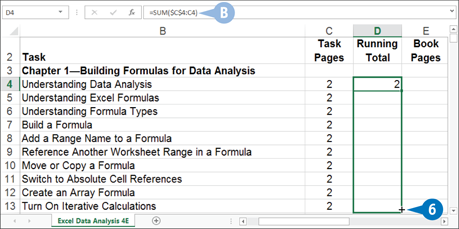
B Excel adjusts the formula.
![]() Copy the formula.
Copy the formula.
Note: See the previous section, Move or Copy a Formula, to learn how to copy a formula.

C Excel preserves the absolute cell references in the copied formula.
Create an Array Formula
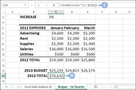
If you find yourself repeating the same formula across a range of cells, you can make your formula-building chores easier and faster by taking advantage of the array formulas in Excel. An array formula is a special formula that generates multiple results. For example, if your worksheet has expense totals in cells C11, D11, and E11, and a budget increase value in cell C3, then you can calculate the new budget values with the following formulas:
=C11 * (1 + $C$3)
=D11 * (1 + $C$3)
=E11 * (1 + $C$3)
Rather than entering these formulas separately, you can enter just a single array formula:
{=C11:E11 * (1 + $C$3)}
The braces, { and }, mark this as an array formula, and Excel enters them automatically.
Create an Array Formula
Create a Multi-Cell Array Formula

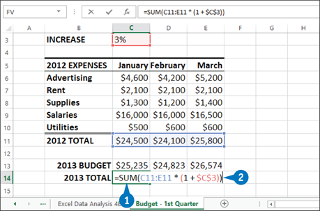
![]() Select the range where you want the formula results to appear.
Select the range where you want the formula results to appear.
![]() Type the array formula.
Type the array formula.
![]() Press Ctrl+Shift+Enter.
Press Ctrl+Shift+Enter.
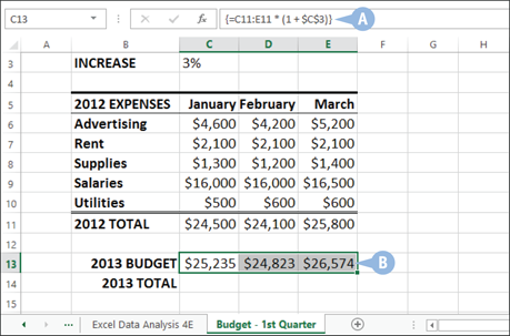
A Excel enters the formula as an array formula and automatically adds braces around it.
B Excel enters the results in the range you selected.
Create a Single-Cell Array Formula
![]() Select the cell where you want the formula result to appear.
Select the cell where you want the formula result to appear.
![]() Type the array formula.
Type the array formula.
![]() Press Ctrl+Shift+Enter.
Press Ctrl+Shift+Enter.
C Excel enters the formula as an array formula and automatically adds braces around it.
D Excel enters the result in the cell you selected.
Turn On Iterative Calculations
In some Excel calculations, you cannot derive the answer directly. Instead, you perform a preliminary calculation, feed that answer into the formula to get a new result, feed the new result into the formula, and so on. Each new result converges on the actual answer. For example, consider a formula that calculates net profit by subtracting the amount paid out in profit sharing from the gross profit. This is not a simple subtraction because the profit sharing amount is calculated as a percentage of the net profit, so you must plug preliminary results back into the formula. This process is called iteration. To perform these types of Excel calculations, you must turn on the iterative calculation feature.
Turn On Iterative Calculations

![]() Build a formula that requires an iterative calculation to solve.
Build a formula that requires an iterative calculation to solve.
A Circular reference arrows appear in the table.
B In the Formulas tab, you can click Remove Arrows to hide the circular reference arrows.
![]() Click the File tab.
Click the File tab.

![]() Click Options.
Click Options.

The Excel Options dialog box appears.
![]() Click Formulas.
Click Formulas.
![]() Click the Enable Iterative Calculation check box (
Click the Enable Iterative Calculation check box (![]() changes to
changes to ![]() ).
).
C If Excel fails to converge on the solution, you can try typing a higher value in the Maximum Iterations text box.
D If you want a more accurate solution, you can try typing a smaller value in the Maximum Change text box.
Note: The Maximum Change value tells Excel how accurate you want your results to be. The smaller the number, the more accurate the calculation, but the iteration takes longer.
![]() Click OK.
Click OK.
Excel performs the iteration.

E The iterated result appears in the formula cell.