8.11 Correlation

In research, as in life, most of the important questions have to do with relationships. An introductory treatment of statistical techniques for experiments would be lopsided without any mention of techniques for investigating relationships among variables. In the previous sections we have compared samples to each other. The reason why we compare them is, of course, that we expect them to differ from each other, probably because they were sampled under different conditions. In other words, we expect that the variables we sample are dependent on other variables. We expect the fuel consumption to vary with the season, the yield of a synthesis to vary with the solvent used, and the hardness of a material to depend on the surface treatment it has undergone. In the t-tests and the ANOVA the independent variables are categorical. This means that they can be labeled but not ordered – the seasons, solvents, or surface treatments have names but not numerical values.

The independent variable is frequently a numerical variable, such as a temperature, a price or a distance. In the remaining parts of this chapter we are going to see how relationships between numerical variables can be investigated. Firstly, we will focus our interest on the strength and direction of the relationship between two variables. Does one variable increase or decrease when the other increases? Such questions are answered using correlation analysis. In the next section, we will see how the relationship between the variables can be described mathematically, introducing a technique called regression modeling.

Correlation is a measure of the strength and direction of the linear association between two variables. Consider two samples of size n that were collected simultaneously, so that each observation in one sample is associated with an observation in the other. They could, for instance, consist of temperatures and pressures in the cylinder of an engine collected during compression. The correlation between two such samples is given by Pearson's correlation coefficient:

(8.8)

where and are the means of the two samples and sx and sy their standard deviations. If the x values tend to be smaller than when the corresponding y values are greater than their mean, and vice versa, the numerator becomes negative. This means that, if y tends to decrease when x increases, the correlation coefficient becomes negative. If x and y tend to vary in the same direction the coefficient becomes positive. Dividing by the standard deviations ensures that the value of the coefficient always lies between −1 and +1. This means that a correlation coefficient that is close to +1 indicates a strong linear association, or correlation, between the samples, whereas a coefficient close to zero indicates a weak correlation or no correlation at all. If the coefficient is close to −1 we say that there is a negative correlation between the samples.

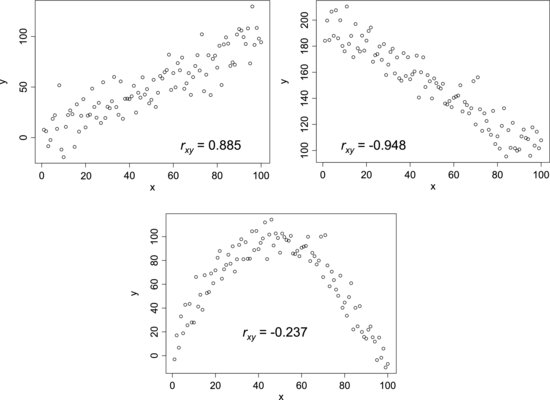
Figure 8.11 shows example scatterplots of x- and y-samples that all have some sort of relationship to each other. Each plot contains a correlation coefficient. The first plot gives an example of strong positive correlation. In this diagram, the points seem to fall along a straight line with positive slope, though there is significant scatter about the line. In the second plot the slope is negative and, consequently, the correlation coefficient indicates a strong negative correlation. Although there is a clear relationship between the variables in the last plot, the coefficient tells us that there is little or no correlation between them. This demonstrates the important fact that a lack of correlation is not the same thing as lack of relationship – only that there is no linear relationship between the variables. For this reason, it is important to always plot the data to avoid the risk that potential relationships among variables remain undiscovered.

Figure 8.11 Examples of data sets where there is some type of relation between the x- and y-variables.

It is also important to point out that, although we use correlation analysis to detect prospective relationships among variables, a high degree of correlation does not prove that there is a direct relationship. If we, for instance, were to compare sales data for sunglasses with the number of people who show symptoms of hay fever, we would probably obtain a positive correlation. The same would be true for a comparison between the occurrence of ski accidents and mitten sales. This does not mean that sunglasses are causing hay fever, or that wearing mittens makes skiing more dangerous. Such apparent relationships may occur by coincidence or, as in this case, if the two variables have a common dependence on a third variable.

The point is that statistical analyses are not a substitute for subject matter knowledge. We should rather use our knowledge of our research fields as much as possible, as this makes it much easier to understand what the data are telling us. Finding a strong correlation is of little use if we cannot explain why the variables should be related to each other.