
8.6 Comparing Two Samples
The one-sample t-test is used to compare one sample to a target value. It is common, for instance, in engineering when a product is developed to meet a certain specification limit. In science, it is more common to compare two samples to each other. Scientists are often interested in assessing the existence of an effect of an environmental condition, a medical procedure, an experimental treatment, or something similar. They do this by comparing samples drawn under different conditions. In such cases there are two scenarios that can occur, since two samples can either be independent of or dependent on each other. If we consider a medical study, we could assign one group of people to a certain treatment and use another group as a control group. This would produce two independent samples. If we instead test the same group before and after receiving the treatment we get two dependent samples, since every person is associated with an observation in each sample. In dependent samples an observation in one sample can be paired with a corresponding observation in the other.
When comparing two independent samples to each other, we use the so-called two-sample t-test. To familiarize ourselves with it we will analyze an experiment where the yield of a chemical synthesis is tested using two different solvents. To maintain the integrity of the significance test the solvent is chosen randomly before each run, in a manner that results in 10 observations for each solvent. The data are given in Table 8.3 and plotted in Figure 8.6. We see that, although sample one has a lower mean yield, there is an overlap between the samples and substantial variation within each set. Let us see if the difference between them is statistically significant.
Figure 8.6 Plot of the data from the synthesis experiment.
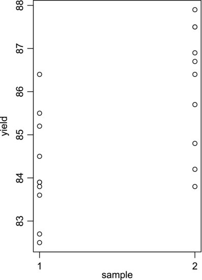
Table 8.3 Data from the synthesis experiment.
| Sample 1 | Sample 2 | |
| 85.2 | 87.5 | |
| 84.5 | 86.7 | |
| 82.5 | 85.7 | |
| 83.9 | 87.9 | |
| 83.6 | 86.9 | |
| 82.7 | 84.8 | |
| 85.5 | 84.2 | |
| 83.8 | 87.5 | |
| 83.9 | 86.4 | |
| 86.4 | 83.8 | |
| Mean: | 84.2 | 86.14 |
The two-sample t-test requires that the samples have equal variances. Say that, based on our experience of similar experiments, we find this to be a reasonable assumption. In such a case it is adequate to estimate the variance by pooling the sums of squares of the two samples, since a larger sample size provides a better estimate. The variance of the first sample is simply its sum of squares divided by its number of degrees of freedom:
(8.3) ![]()
and the variance of the second sample is determined in the same way. If these two variances are reasonably equal they may be combined to provide a pooled estimate of the variance:
(8.4) ![]()
Here, we have simply added the sums of squares in the nominator and the numbers of degrees of freedom in the denominator.
We want to determine if the difference between the means of the two samples is significantly different from a hypothetical difference δ. Our observed t-value then becomes:
where the denominator is the estimated standard deviation of the difference between the means. (You may convince yourself of this by using the additive property of the variances of the two means.) Comparing with Equation 8.1 you will find that Equation 8.5 is exactly analogous but instead of sample and population means we are now using differences between sample and population means.
The null hypothesis assumes that the two solvents produce equal results and that any difference between them is due to random error, so:
(8.6) ![]()
Note that the null hypothesis, as always, contains an equals sign.
Using δ = 0 in Equation 8.5 we obtain a tobs of −3.16. To see if this is a statistically significant result we need a critical t-value. Just as before, it may be read from the table of the t-distribution in the Appendix. With 18 degrees of freedom and α/2 = 0.025 (that is, for a two-sided test) we obtain a tcrit of 2.101. Since tobs is farther from zero than ±2.101 we conclude that the result is significant – the data support the conclusion that there is a difference between the samples.
An alternative way of making the significance test is to calculate the p-value directly, using the Excel worksheet function TDIST. It requires three input arguments: tobs, the number of degrees of freedom, and the number of tails of the test. Writing “=TDIST(3.16;18;2)” into a worksheet cell returns a p-value of 0.005. Being much lower than our α of 0.05, this discredits the null hypothesis.
Let us look at another example in order to demonstrate how dangerous it can be to follow cookbook recipes without reflecting over the nature of the data. Recall the team of researchers who, in Chapter 7, wanted to investigate how a certain diet affected the blood pressure of healthy people. They measured the systolic blood pressure of their 15 test persons before starting the diet. The values, in mm Hg, are given for persons 1–15 below. They are rounded to the nearest integer to help us concentrate on the essentials:
![]()
After 15 days of diet, the blood pressures were measured again:
![]()
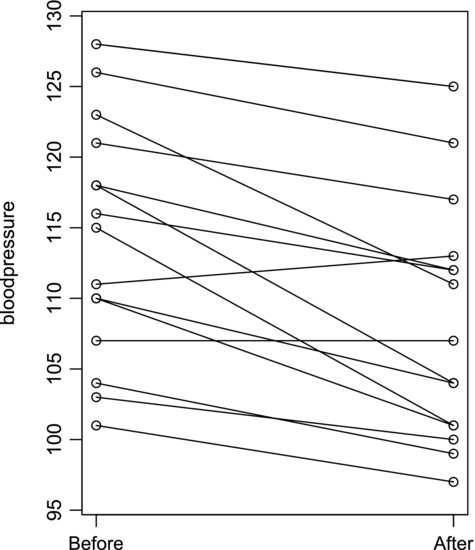
Again, these values are ordered from test person 1 to test person 15. Before continuing the analysis we examine them graphically in Figure 8.7, which shows a clear tendency for the blood pressure to drop after the diet. Only one person shows an increase and another person's remains the same after the test.
Figure 8.7 Blood pressure data.
We will now attempt to investigate the significance of this tendency by the two-sample t-test. The null hypothesis is that there is no difference between the samples, or that δ = 0. The mean blood pressures before and after the diet are 114.1 and 108.3 mm Hg, respectively. Using these values in Equation 8.5 we obtain tobs = −1.89. We read the critical t-value from the table of the t-distribution in the Appendix, which states that tcrit = 2.048 for α/2 = 0.025 (two-sided test) and 28 degrees of freedom. As tobs is less extreme than tcrit the null hypothesis is supported: there seems to be no difference between the samples.
How can this be, when Figure 8.7 clearly shows that the blood pressure decreases after the diet? The reason for this counter-intuitive result is simply that we have used the wrong test for these data. Since the same persons are associated with one observation in each sample, the samples are dependent. In such cases we should use what is called the paired t-test, which will be explained in the remainder of this section. It will also become clear why the paired t-test works better in this case.
All the theory needed to understand the paired t-test has already been covered, since it is simply a special case of the one-sample t-test. The first step is to calculate the change in blood pressure that each test person experiences as a result of the diet, just as we did at the end of Chapter 7. These are given in the third column of Table 8.4. Looking at the standard deviations of the columns, which are given at the bottom of the table, we see that the “difference” column displays less variation than the original data in the “before” and “after” columns. The reason is that the original data contains variation between the individuals. Taking the difference between each person's value before and after the diet we eliminate this source of variation. What is left is each person's response to the diet, irrespective of his or her original blood pressure. In short, the paired t-test removes variation that is not due to the experimental treatment and highlights the effect of the treatment.
Table 8.4 Blood pressure data recorded before and after the diet, as well as the difference between them.
The difference column in Table 8.4 can now be treated as a single sample. We obtain the observed t-value using Equation 8.1, where ![]() now corresponds to the mean difference and μ to the hypothetical difference, which is zero. The mean difference in blood pressure is −5.8 mm Hg, the sample standard deviation is 4.7 mm Hg, and the number of observations is 15. Plugging these numbers into Equation 8.1 yields a tobs of −4.62, which is much farther from the hypothesized mean of zero than our tcrit which, according to the t-table in the Appendix, is 2.145. Alternatively, the p-value returned from the worksheet function TDIST is 0.0004. As opposed to the result of our erroneous use of the two-sample t-test with these data, this analysis is capable of detecting the effect that the diet has on the blood pressure. The reason that the paired t-test is more sensitive is that it removes the variation between the individuals, but this is only possible when the samples are dependent.
now corresponds to the mean difference and μ to the hypothetical difference, which is zero. The mean difference in blood pressure is −5.8 mm Hg, the sample standard deviation is 4.7 mm Hg, and the number of observations is 15. Plugging these numbers into Equation 8.1 yields a tobs of −4.62, which is much farther from the hypothesized mean of zero than our tcrit which, according to the t-table in the Appendix, is 2.145. Alternatively, the p-value returned from the worksheet function TDIST is 0.0004. As opposed to the result of our erroneous use of the two-sample t-test with these data, this analysis is capable of detecting the effect that the diet has on the blood pressure. The reason that the paired t-test is more sensitive is that it removes the variation between the individuals, but this is only possible when the samples are dependent.