
8.7 Analysis of Variance (ANOVA)
So far we have compared one sample to a standard (the one-sample t-test) and two samples to each other (the two-sample and paired t-tests). Sometimes we want to find out if there is a difference between several samples. A technique that is useful in such cases is the so-called Analysis of Variance, or ANOVA for short. It is based on breaking the variation in the data down into several parts.
It may seem confusing at first that ANOVA, which is a technique for comparing three or more sample means, is based on the variation in the data. The best way to understand how this works is probably to work through an example. We will compare three different surface treatment methods for steel. An experiment is performed where steel parts are surface treated and subjected to abrasive wear tests. After the tests the weight loss is measured. We are interested in finding out if the surface treatments affect the amount of wear. The measurement data are given in Table 8.5, where the columns represent the treatments (A, B and C) and the rows correspond to five different metal parts exposed to each treatment. In total, 15 parts are used in this experiment. Below the table, the mean weight loss is given for each treatment and for the experiment as a whole (grand mean). Also, the differences between the grand mean and the treatment means are given. It is important to point out that the metal parts are allocated randomly to the treatments and tested in random order, to ensure the integrity of the significance test that we are about to perform.
Table 8.5 Measurement data from abrasive wear tests in the surface treatment experiment.
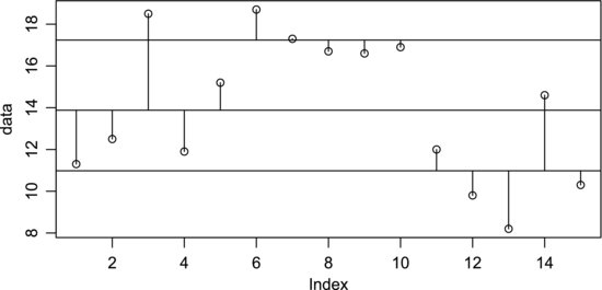
It cannot be stated often enough that it is always appropriate to plot the data before proceeding further with the analysis. The three samples are shown in Figure 8.8, where the horizontal line represents the grand mean. The first five points represent sample A, the next five points sample B, and the last points sample C. Each point is connected to the grand mean with a vertical line that represents the deviation from the grand mean. It is quite easy to see that the samples have different means, but at what level of significance? There is substantial variation within each treatment and the samples are partially overlapping. Figure 8.9 shows the same data but the points are now connected to their sample means, represented by the three horizontal lines. We can now make the important observation that the average deviations from the sample means are smaller than the average deviation from the grand mean. We will return to this observation after going through the analysis.
Figure 8.8 Abrasive wear data plotted in relation to the grand mean. The first five points represent sample A, the next five sample B, and the last five sample C.
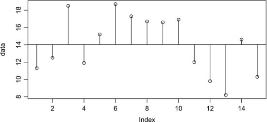
Figure 8.9 Abrasive wear data plotted in relation to the respective sample means.
To determine the total variation in the data we will calculate the deviations from the grand mean. These are given in the matrix D in Table 8.6 and are just each element in Table 8.5 minus the grand mean. The first row contains −2.7 = 11.3 − 14, 4.7 = 18.7 − 14, and so on. The total variation is then decomposed into a part T due to the treatments and a residual part R. T contains the treatment means minus the grand mean. It represents the variation between the treatments. Since R represents the variation that is not due to the treatments, it contains the elements of Table 8.5 minus the treatment means. This is the variation within the treatments or, in other words, the experimental error. Note that if you add the elements of T and R you obtain the elements in D.
Table 8.6 Abrasive wear data broken down into several parts.
The data in Table 8.6 will now be used to construct what is usually called an ANOVA table, given in Table 8.7. The variation is divided into two sources: that due to the treatments (variation between samples) and that due to experimental error (variation within samples). The last source is just the sum of the others, or the total variation. We will start by looking at the second column, which contains the sums of squares, SS, from the three sources. SSR is due to the experimental error and is calculated by simply squaring all the elements of R and summing them:
(8.7) ![]()
Table 8.7 ANOVA table for the abrasive wear tests.
Similarly, SST, which is due to the treatments, is all the elements of T squared and summed. The total sum of squares, SSD, is the elements of D squared and summed. You may note that it is also given by SST + SSR, as the sums of squares are additive.
The first column of Table 8.7 contains the numbers of degrees of freedom for each source of variation. Recall from Chapter 7 that they are given by the number of observations and the number of population parameters that are estimated from them. The total variation is associated with the matrix D. Since it is the difference between each observation and the grand mean it has n – 1 = 14 degrees of freedom. The error is associated with the matrix R, where treatment means have been calculated from the five observations in each column. As there are three treatment means, it has 15 – 3 = 12 degrees of freedom. Finally, T, which contains the differences between the treatment means and the grand mean, represents the variation due to the treatments. There are three treatments, so it has 3 – 1 = 2 degrees of freedom. Note that the total number of degrees of freedom is the sum of the others.
We now have all the elements needed to calculate the mean squares, MS, in the third column. These are just each sum of squares, SS, divided by its number of degrees of freedom, ν. They therefore have the form of variances. The error mean square is actually the unbiased estimate of the error variance, σ2, that was introduced in Box 6.1. It therefore says something about the precision in the data. If the treatments do not produce different results (that is, if the treatment means are equal), it can be shown also that the treatment mean square is an unbiased estimate of σ2 [2]. In this case, Table 8.7 shows that the treatments produce a larger mean square than the error does. Comparing these two components of the variation thereby reveals that there is a difference between the treatment means. The question is if it is statistically significant.
To answer this question we need a suitable significance test. The null hypothesis to be tested is that the treatments do not have an effect, which is equivalent to saying that both the treatment and error mean squares are estimates of σ2. The equality of two variances is tested using the F-test, since ratios of variances can be shown to follow a so-called F-distribution. The interested reader can find out why this is so by reading, for example, Box, Hunter, and Hunter [3]. Here we will settle with just stating this as a fact. The F-test follows the same basic procedure as the t-test. We will compare an observed F-value, representing our data, to a critical F-value, representing our α-value. This will indicate the potential effect of the treatment.
To get our observed F-value of 9.46, we simply divide the mean square of the treatment by that of the error. This is to be compared to the critical F-value for the 95% confidence level, which can be read from a table of the F-distribution. The procedure is exactly analogous to the t-test: if our observed F-value is more extreme than the critical one, the null hypothesis is discarded. In this example, however, we will proceed directly to calculating a p-value as this is so easily done using the Excel function FDIST.
The required input arguments are the observed F-value and the number of degrees of freedom of the two mean squares. Thus, writing “=FDIST(9.46;2;12)” into an Excel worksheet and pressing enter returns the p-value, 0.003. This is the probability of obtaining our data, or something more extreme, under the null hypothesis that the treatments have no effect on the result. The outcome is clearly significant at the 95% confidence level. The null hypothesis is thereby strongly discredited. Our data support that that the surface treatments produce different amounts of weight loss. Remember the mnemonic: “if p is low, H0 should go!’
In summary, we have used the ANOVA to judge the significance of the difference between the sums of squares computed from the grand mean and from the individual treatment means. To put it simply, if the means are significantly different, the treatment sum of squares is smaller than the overall sum of squares [4]. This is actually what we saw graphically in Figures 8.8 and 8.9 when we noted that the average deviation from the sample means were smaller than the average deviation from the grand mean.
The ANOVA is used to compare three or more sample means to each other. It is worth mentioning that if you were to try to compare two sample means by ANOVA you would get exactly the same result as from a two-sample t-test. In fact, it is a good exercise to convince yourself of this by doing it.
It may also be worth mentioning that, if you try to reconstruct the entries in the ANOVA table using the numbers in Tables 8.4 and 8.5, you will get a slightly different result as they have been rounded to one decimal point.
| O | N | N+P |
| 12.25 | 11.25 | 13.00 |
| 11.50 | 12.75 | 13.50 |
| 10.75 | 11.75 | 12.50 |
| 10.50 | 12.00 | 12.25 |
| O: organic; N: nitrogen; N+P: nitrogen and phosphorus | ||