7.5 The Central Limit Effect

How can it be that the normal distribution holds such a central position in statistics? There are many other ways that data may be distributed. If we roll a six-sided die, for example, the probability of each score is 1/6. In other words, the frequency distribution of the scores is completely flat, far from the bell-shaped Gaussian curve. The roll of a die is a relatively simple process, however. Measurements are more complex. The error in measurement data is usually combined from a large number of component errors. When discussing the synthesis experiment earlier, we mentioned a few sources of error that could contribute to the overall error: variations in reactant concentrations, mixture homogeneity, temperature, as well as measurement precision and operator repeatability. There are numerous other potential error sources, such as the purity of the reactants. We do not know which distributions these individual errors follow but due to the central limit effect we know something about how the combination of a large number of such errors is distributed. This effect makes the mean of a number of random variables follow a normal distribution when the number of variables becomes large, almost regardless of how each variable is distributed.

Figure 7.9 Histograms showing the scores from throwing a single die (top), two dice (middle) and ten dice (bottom). (When several dice are thrown the mean score is calculated.)

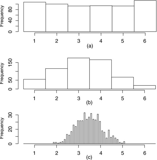
The most simple and effective way to demonstrate the central limit effect is perhaps by tumbling dice. As we have mentioned, we expect the frequency distribution of scores from tumbling a true die to be flat. The top histogram in Figure 7.9 shows the result of 600 throws of a single die. The frequency of each score is approximately 100, or one sixth of the number of throws, just as expected. The mean score is 3.5. What happens if we throw two dice simultaneously and calculate the average score from each throw? The middle histogram shows that the distribution now takes on a pointed appearance; it has lost its flatness. Intuitively, this can be understood by noting that there is only one combination of scores from two dice that produces the lowest possible mean score, which is one. The same is true about the highest possible score, six, whereas there are a large number of combinations that produce a mean score close to 3.5. Since each combination occurs with the same probability the frequency becomes highest around the mean. Looking at the bottom histogram, which results from throwing ten dice simultaneously and calculating the mean score, we see that the distribution approaches the Gaussian curve. With so many dice the probability of each unique combination becomes so low that 600 throws were not enough, in this case, to produce a single occurrence of neither the lowest nor the highest possible score.

This demonstrates how the mean of a large number of random variables tends to follow a normal distribution, even though their individual distributions may deviate significantly from normality. This is a remarkable and highly useful effect. The reason that the normal distribution is so important is that many natural processes are affected by a wealth of factors and subprocesses. Also, our measurement systems are affected by a large number of random errors. In real-world experimentation, therefore, it is often reasonable to assume that the experimental error follows a normal distribution. An important condition for this to be true is that the contribution from each component of the variation is of the same order of magnitude. If one component dominates over the others we can no longer adduce the central limit effect and assume that the error is normally distributed.

The central limit effect is stated mathematically by the central limit theorem, which will be used for calculating confidence intervals later in this chapter. Let us consider a variable X that follows an unknown distribution with mean μ and standard deviation σ. Imagine that we take samples of Xs, each containing n observations. The central limit theorem states that, when n becomes large, the means of these samples will tend to follow a distribution that:

• has mean μ;
• has standard deviation
• is normally distributed.

Let us reflect on what this means. The last point is the central limit effect, which we illustrated with the dice. The first point states that we can estimate the population mean by calculating the mean of the sample. The second point states that we obtain a better estimate of the population mean by using a larger sample. This is because the standard deviation of the estimate decreases when n increases, exactly as we saw in the dice data: when the sample size increased from one to two, and later to ten, the estimated mean remained 3.5 but the precision of the estimate increased. The decrease in standard deviation with increasing sample size reflects a decreased uncertainty in the estimate. I suggest that you read this paragraph repeatedly until you are sure that you understand what it says, because the central limit theorem is one of the most important things to understand in statistics.

Remember that the normal distribution is an ideal concept – in the real world we seldom encounter data that exactly follow this distribution. Fortunately, most statistical techniques only require approximate normality to be useful. For example, the techniques for estimating and comparing means that will be introduced in the next chapter are robust to non-normality.