
CHAPTER 9
Interacting with the Physical Environment
In this chapter, you will learn how to build on your knowledge of GPIO and bus interfacing. In particular, you can combine hardware and software to provide the Beagle boards with the ability to interact with their physical environments in the following three ways: First, by controlling actuators such as motors, the board can affect its environment, which is important for applications such as robotics and home automation. Second, the board can gather information about its physical environment by communicating with sensors. Third, by interfacing to display modules, the board can present information. This chapter explains how each of these interactions can be performed. Physical interaction hardware and software provides you with the capability to build advanced projects, such as to build a robotic platform that can sense and interact with its environment. The chapter finishes with a discussion on how you can build your own C/C++ code libraries and interact with them to build highly scalable projects.
EQUIPMENT REQUIRED FOR THIS CHAPTER:
- Beagle board, DMM, and oscilloscope
- DC motor and H-bridge interface board
- Stepper motor, EasyDriver interface board, and a 5 V relay
- Op-amps (LM358, MCP6002/4), diodes, resistors, 5 V relay
- TMP36 temperature sensor and Sharp infrared distance sensor
- MCP3208 SPI ADC, op-amp (MCP6002/4), diodes, and resistors
- LCD character display module
- MAX7219 seven-segment display module
- ADXL335 analog three-axis accelerometer
Further details on this chapter are available at www.exploringbeaglebone.com/chapter9/.
Interfacing to Actuators
Electric motors can be controlled by the Beagle boards to make physical devices move or operate. They convert electrical energy into mechanical energy that can be used by devices to act upon their surroundings. A device that converts energy into motion is generally referred to as an actuator. Interfacing a board to actuators provides a myriad of application possibilities, including robotic control, home automation (e.g., control of locks, controlling blinds), camera control, unmanned aerial vehicles (UAVs), 3D printer control, and many more.
Electric motors typically provide rotary motion around a fixed axis, which can be used to drive wheels, pumps, belts, electric valves, tracks, turrets, robotic arms, and so on. In contrast to this, linear actuators create movement in a straight line, which can be useful for position control in computer numerical control (CNC) machines and 3D printers. In some cases, they convert rotary motion into linear motion using a screw shaft that translates a threaded nut along its length as it rotates. In other cases, a solenoid moves a shaft linearly through the magnetic effects of an electric current.
Three main types of motors are commonly used with embedded Linux boards: servo motors, DC motors, and stepper motors. Table 9-1 provides a summary comparison of these motor types. Interfacing to servo motors (also known as precision actuators) through the use of PWM outputs is discussed in Chapter 6, so this section focuses on interfacing to DC motors and stepper motors.
Table 9-1: Summary Comparison of Common Motor Types
| SERVO MOTOR | DC MOTOR | STEPPER MOTOR | |
| Typical application | When high torque, accurate rotation is required. | When fast, continuous rotation is required. | When slow and accurate rotation is required. |
| Control hardware | Position is controlled through PWM. No controller required. May require PWM tuning. | Speed is controlled through PWM. Additional circuitry required to manage power requirements. | Typically requires a controller to energize stepper coils. A Beagle board can perform this role, but an external controller is preferable and safer. |
| Control type | Closed-loop, using a built-in controller. | Typically closed-loop using feedback from optical encoders. | Typically open-loop, as movement is precise and steps can be counted. |
| Features | Known absolute position. Typically, limited angle of rotation. | Can drive large loads. Often geared to provide high torque. | Full torque at standstill. Can rotate a large load at low speeds. Tendency to vibrate. |
| Example applications | Steering controllers, camera control, and small robotic arms. | Mobile robot movement, fans, water pumps, and electric cars. | CNC machines, 3D printers, scanners, linear actuators, and camera lenses. |
The applications discussed in this section often require a secondary power supply, which could be an external battery pack in the case of a mobile platform or a high-current supply for powerful motors. The boards need to be isolated from these supplies; as a result, generic motor controller boards are described here for interfacing to DC motors and stepper motors. Circuitry is also carefully designed for interfacing to relay devices.
DC Motors
DC motors are used in many applications, from toys to advanced robotics. They are ideal motors to use when continuous rotation is required, such as in the wheels of an electric vehicle. Typically, they have only two electrical terminals to which a voltage is applied. The speed of rotation and the direction of rotation can be controlled by varying this voltage. The tendency of a force to rotate an object around its axis is called torque, and for a DC motor, torque is generally proportional to the current applied.
The higher the gear ratio, the slower the rotation speed, and the higher the stall torque. For example, the DC motor in Figure 9-1(a) has a no-load speed of 80 revolutions per minute (rpm) and a stall torque of 250 oz·in (18 kg·cm).1 Similarly, if a 70:1 gear ratio is used, the rotation speed becomes 150 rpm, but the stall torque reduces to 200 oz·in (14.4 kg·cm). The DC motor in Figure 9-1(a) has a free-run current of 300 mA at 12 V, but it has a stall current of 5 A—a large current that must be factored into the circuit design.
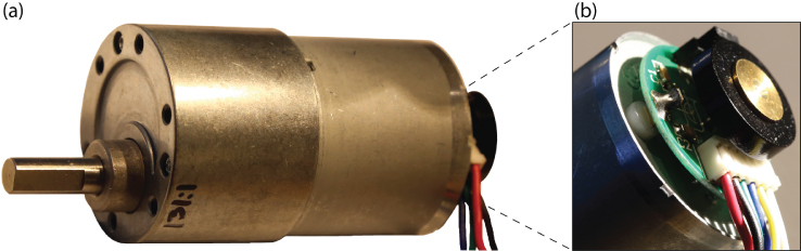
Figure 9-1: (a) A 12 V DC motor with an integrated 131¼:1 gearbox ($40), and (b) an integrated counts per revolution (CPR) Hall Effect sensor shaft encoder
Most DC motors require more current than the Beagle boards can supply; therefore, you might be tempted to drive them from your board by simply using a transistor or FET. Unfortunately, this will not work well because of a phenomenon known as inductive kickback, which results in a large voltage spike that is caused by the inertia of current flowing through an inductor (i.e., the motor's coil windings) being suddenly switched off. Even for modest motor power supplies, this large voltage could exceed 1 kV for a short period of time. The FETs discussed in Chapter 4 cannot have a drain-source voltage of greater than 60 V and will therefore be damaged by such large voltage spikes.
One solution is to place a Zener diode across the drain-source terminals of the FET (or collector-emitter of a transistor). The Zener diode limits the voltage across the drain-source terminals to that of its reverse breakdown voltage. The downside of this configuration is that the ground supply has to sink a large current spike, which could lead to the type of noise in the circuit that is discussed in Chapter 4. With either of these types of protection in place, it is possible to use a Beagle board PWM output to control the speed of the DC motor. With a PWM duty cycle of 50 percent, the motor will rotate at half the speed that it would if directly connected to the motor supply voltage.
The DC motor in Figure 9-1 has a 64 counts per revolution (CPR) quadrature encoder that is attached to the motor shaft, which means there are 64 × 131.25 = 8,400 counts for each revolution of the geared motor shaft. Shaft encoders are often used with DC motors to determine the position and speed of the motor. For example, the encoder has an output as illustrated in Figure 9-2(a) when rotating clockwise and Figure 9-2(b) when rotating counterclockwise. The frequency of the pulses is proportional to the speed of the motor, and the order of the rising edges in the two output signals describes the direction of rotation. Note that the Hall Effect sensor must be powered, so four of the six motor wires are for the encoder: A output (yellow), B output (white), encoder power supply (blue), GND (green). The remaining two wires are for the motor power supply (red and black).
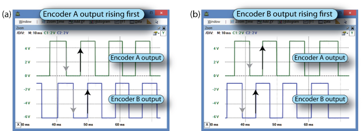
Figure 9-2: The output from the shaft encoder in Figure 9-1(b) when rotating: (a) clockwise, and (b) counterclockwise
An alternative to this configuration is to place a Zener diode across the drain-source terminals of the FET (or collector-emitter of a transistor). The Zener diode limits the voltage across the drain-source terminals to that of its reverse breakdown voltage. The downside of this alternative configuration is that the ground supply has to sink a large current spike, which could lead to the type of noise in the circuit that is discussed in Chapter 4. With either of these types of protection in place, it is possible to use a Beagle board PWM output to control the speed of the DC motor. With a PWM duty cycle of 50 percent, the motor will rotate at half the speed that it would if directly connected to the motor supply voltage.
For bidirectional motor control, a circuit configuration called an H-bridge can be used, which has a circuit layout in the shape of the letter H, as illustrated in Figure 9-3. Notice that it has Zener diodes to protect the four FETs. To drive the motor in a forward (assumed to be clockwise) direction, the top-left and bottom-right FETs can be switched on. This causes a current to flow from the positive to the negative terminal of the DC motor. When the opposing pair of FETs is switched on, current flows from the negative terminal to the positive terminal of the motor and the motor reverses (turns counterclockwise). The motor does not rotate if two opposing FETs are switched off (open circuit).

Figure 9-3: Simplified H-bridge description
Four Beagle board PWM header pins could be connected to the H-bridge circuit, but particular care must be taken to ensure that the two FETs on the left side or right side of the circuit are not turned on at the same time, as this would result in a large current (shoot-through current)—the motor supply would effectively be shorted (VM
to GND). As high-current capable power supplies are often used for the motor power supply, this is dangerous, as it could even cause a power supply or a battery to explode! An easier and safer approach is to use an H-bridge driver that has already been packaged in an IC, such as the SN754410, a quadruple high-current half-H driver, which can drive 1 A at 4.5 V to 36 V per driver (see tiny.cc/beagle901).
Driving Small DC Motors (up to 1.5 A)
There are many more recently introduced drivers that can drive even larger currents using smaller package sizes than the SN754410. In this example, a DRV8835 dual low-voltage motor driver carrier on a breakout board ($4) from www.pololu.com is used, as illustrated in Figure 9-4. The DRV8835 itself is only 2 mm × 3 mm in dimension and can drive 1.5 A (max) per H-bridge at a motor supply voltage up to 11 V. It can be driven with logic levels of 2 V to 7 V, which enables it to be used directly with a Beagle board.
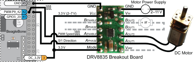
Figure 9-4: Driving a DC motor using an example H-Bridge driver breakout board
The DRV8835 breakout board can be connected to the BeagleBone as illustrated in Figure 9-4. This circuit uses four pins from the BeagleBone:
- P9_3 provides a 3.3 V supply for the control logic circuitry.
- P9_45 provides a GND for the logic supply circuitry.
- P9_42 provides a PWM output from the BeagleBone that can be used to control the rotation speed of the motor, as it is connected to the AENABLE input on the DRV8835.
- P9_41 provides a GPIO output that can be used to set whether the motor is rotating clockwise or counterclockwise, as it is connected to the APHASE input.
The motor power supply voltage is set according to the specification of the DC motor that is chosen. By tying the Mode pin high, the DRV8835 is placed in PHASE/ENABLE mode, which means that one input is used for direction, and the other is used for determining the rotation speed.
Controlling a DC Motor Using sysfs
With a circuit wired as shown in Figure 9-4, the DC motor can be controlled using sysfs. In this example, P9_41 (GPIO3_20 = 116) is connected to the APHASE
input. Therefore, this pin can be enabled, and the motor's direction of rotation can be controlled using the following:
debian@ebb:~$ config-pin -a P9_41 outdebian@ebb:~$ config-pin -q P9_41P9_41 Mode: gpio Direction: out Value: 0debian@ebb:~$ cd /sys/class/gpio/gpio116debian@ebb:/sys/class/gpio/gpio116$ lsactive_low device direction edge label power subsystem uevent valuedebian@ebb:/sys/class/gpio/gpio116$ echo out > directiondebian@ebb:/sys/class/gpio/gpio116$ echo 1 > valuedebian@ebb:/sys/class/gpio/gpio116$ echo 0 > value
The speed of the motor can be controlled using a BeagleBone PWM output. The overlays can be loaded, and the motor can be controlled using the PWM overlay that is associated with P9_42, as follows:
debian@ebb:~$ config-pin -l P9_42default gpio gpio_pu gpio_pd gpio_input spi_cs spi_sclk uart pwm pru_ecapdebian@ebb:~$ config-pin -a P9_42 pwmdebian@ebb:~$ config-pin -q P9_42 pwmP9_42 Mode: pwmdebian@ebb:~$ cd /sys/class/pwmdebian@ebb:/sys/class/pwm$ lspwmchip0 pwmchip1 pwmchip3 pwmchip5 pwmchip6
As described in Chapter 6, P9_42 is connected to ECAP0, which is mapped to the pwmchip0 device. This device must be enabled and configured, whereupon modifying the duty cycle will control the rotation speed of the motor.
debian@ebb:/sys/class/pwm$ cd pwmchip0debian@ebb:/sys/class/pwm/pwmchip0$ lsdevice export npwm power subsystem uevent unexportdebian@ebb:/sys/class/pwm/pwmchip0$ echo 0 > exportdebian@ebb:/sys/class/pwm/pwmchip0$ lsdevice export npwm power pwm-0:0 subsystem uevent unexportdebian@ebb:/sys/class/pwm/pwmchip0$ cd pwm-0:0/debian@ebb:/sys/class/pwm/pwmchip0/pwm-0:0$ lscapture device duty_cycle enable period polarity power subsystem ueventdebian@ebb:/sys/class/pwm/pwmchip0/pwm-0:0$ sudo sh -c "echo 4000 > period"debian@ebb:/sys/class/pwm/pwmchip0/pwm-0:0$ sudo sh -c "echo 1000 > duty_cycle"debian@ebb:/sys/class/pwm/pwmchip0/pwm-0:0$ cat polaritynormaldebian@ebb:/sys/class/pwm/pwmchip0/pwm-0:0$ sudo sh -c "echo 1 > enable"debian@ebb:/sys/class/pwm/pwmchip0/pwm-0:0$ sudo sh -c "echo 2000 > duty_cycle"debian@ebb:/sys/class/pwm/pwmchip0/pwm-0:0$ sudo sh -c "echo 4000 > duty_cycle"debian@ebb:/sys/class/pwm/pwmchip0/pwm-0:0$ sudo sh -c "echo 0 > enable"
Here, the PWM frequency is set to 250 kHz, and the duty cycle is adjusted from 25 percent to 50 percent and then to 100 percent, changing the rotation speed of the motor accordingly. As with servo motors, DC motors should be controlled with the PWM polarity set to normal (as opposed to inversed) so that the duty period represents the time when the pulse is high rather than low. The direction of rotation can be adjusted at any stage using the gpio116 sysfs directory.
Driving Larger DC Motors (Greater than 1.5 A)
The Pololu Simple Motor Controller family ($30–$55), illustrated in Figure 9-5(a), supports powerful brushed DC motors with continuous currents of up to 23 A and maximum voltages of 34 V. It supports USB, TTL serial, analog, and hobby radio-control (RC) PWM interfaces. The controller uses 3.3 V logic levels, but it is also 5 V tolerant.

Figure 9-5: (a) The Pololu Simple Motor Controller, and (b) the associated motor configuration tool
Despite its name, this is an advanced controller that can be configured with settings such as maximum acceleration/deceleration, adjustable starting speed, electronic braking, over-temperature threshold/response, etc., which makes it a good choice for larger-scale robotic applications. The controller can be configured using a Windows GUI application, as illustrated in Figure 9-5(b), or by using a Linux command-line user interface. The Windows configuration tool can also be used to monitor motor temperature and voltage conditions and control the speed settings, braking, PWM, communications settings, and so on, over USB, even while the motor is connected to the Beagle board with a TTL serial interface.
The 3.3 V TTL serial interface is likely the best option for embedded applications, as it can be used directly with a UART device. A UART device can be utilized for communication, as described in Chapter 8.
The Simple Motor Controller can be configured to be in a serial ASCII mode, whereupon it can be controlled using a UART device from the Beagle board with minicom. For example, with ASCII mode enabled and a fixed baud rate of 115,200 (8N1) set in the Input Settings tab (see Figure 9-5(b)), the board can connect directly to the motor controller and issue text-based commands to control the motor, such as V (version), F (forward), B (brake), R (reverse), GO (exit safe-start mode), X (stop), and so on. See the comprehensive manual for the full list of commands (tiny.cc/beagle902).
debian@ebb:/dev$ minicom -b 115200 -o -D /dev/ttyO4V!161 01.04GO.F 50%.B?GO.R 25%.
The Simple Motor Controller can also be controlled directly using the C/C++ UART communications code that is described in Chapter 8. The configuration tool can be used to set the serial TTL mode to be Binary mode with a baud rate of 115,200. Assuming the motor controller is attached to /dev/ttyO4 (as shown previously), the motor.c code example in the /chp09/simple/ directory can be used to control the motor directly.
debian@ebb:~/exploringbb/chp09/simple$ gcc motor.c -o motordebian@ebb:~/exploringbb/chp09/simple$ ./motorStarting the motor controller exampleError status: 0x0000Current Target Speed is 0.Setting Target Speed to 3200.
Controlling a DC Motor Using C++
A C++ class that you can use to control a DC motor is available in the GitHub repository. The constructor expects a named PWM input, which has already been configured via sysfs, and a GPIO object or GPIO number. Listing 9-1 displays the C++ header file for the DCMotor class.
Listing 9-1: library/motor/DCMotor.h
class DCMotor {public:enum DIRECTION{ CLOCKWISE, ANTICLOCKWISE };private:…public:DCMotor(PWM *pwm, GPIO *gpio);DCMotor(PWM *pwm, int gpioNumber);DCMotor(PWM *pwm, GPIO *gpio, DCMotor::DIRECTION direction);DCMotor(PWM *pwm, int gpioNumber, DCMotor::DIRECTION direction);DCMotor(PWM *pwm, GPIO *gpio, DCMotor::DIRECTION direction, float speedPercent);DCMotor(PWM *pwm, int gpioNumber, DCMotor::DIRECTION direction, float speedPercent);virtual void go();virtual void setSpeedPercent(float speedPercent);virtual float getSpeedPercent() { return this->speedPercent; }virtual void setDirection(DIRECTION direction);virtual DIRECTION getDirection() { return this->direction; }virtual void reverseDirection();virtual void stop();virtual void setDutyCyclePeriod(unsigned int period_ns);virtual ~DCMotor();};
An example application that uses the DCMotor class is provided in Listing 9-2. Notice that the header file is in the motor subdirectory.
Listing 9-2: /chp09/dcmotor/DCMotorApp.cpp
#include <iostream>#include <unistd.h>#include "motor/DCMotor.h"using namespace std;using namespace exploringBB;int main(){cout << "Starting EBB DC Motor Example" << endl;DCMotor dcm(new PWM("pwmchip0/pwm-0:0/"), 116); // exports GPIO116dcm.setDirection(DCMotor::ANTICLOCKWISE);dcm.setSpeedPercent(50.0f); //make it clear that a float is passeddcm.go();cout << "Rotating Anticlockwise at 50% speed" << endl;usleep(5000000); //sleep for 5 secondsdcm.reverseDirection();cout << "Rotating clockwise at 50% speed" << endl;usleep(5000000);dcm.setSpeedPercent(100.0f);cout << "Rotating clockwise at 100% speed" << endl;usleep(5000000);dcm.stop();cout << "End of EBB DC Motor Example" << endl;}
The build script assumes that the example application source is in /exporingbb/chp09/dcmotor/ and that the shared library and header files are in the directory /exploringbb/library/. This conforms to the directory structure of the GitHub repository. The code can be built using the build script that is in the dcmotor directory and executed using the following:
debian@ebb:~/exploringbb/chp09/dcmotor$ more build#!/bin/bashg++ DCMotorApp.cpp ../../library/libEBBLibrary.so -o DCApp -I "../../library"debian@ebb:~/exploringbb/chp09/dcmotor$ ./builddebian@ebb:~/exploringbb/chp09/dcmotor$ lsDCApp DCMotorApp.cpp builddebian@ebb:~/exploringbb/chp09/dcmotor$ sudo ./DCAppStarting EBB DC Motor ExampleRotating Anti-clockwise at 50% speedRotating clockwise at 50% speedRotating clockwise at 100% speedEnd of EBB DC Motor Example
At the end of this chapter a description is provided that shows how to build code into dynamic libraries, such as libEBBLibrary.so. This enables you to alter the library to suit your requirements.
Stepper Motors
Unlike DC motors, which rotate continuously when a DC voltage is applied, stepper motors normally rotate in discrete fixed-angle steps. For example, the stepper motor that is used in this chapter rotates with 200 steps per revolution and therefore has a step angle of 1.8°. The motor steps each time a pulse is applied to its input, so the speed of rotation is proportional to the rate at which pulses are applied.
Stepper motors can be positioned accurately, as they typically have a positioning error of less than 5 percent of a step (i.e., typically ±0.1°). The error does not accumulate over multiple steps, so stepper motors can be controlled in an open-loop form, without the need for feedback. Unlike servo motors, but like DC motors, the absolute position of the shaft is not known without the addition of devices like rotary encoders, which often include an absolute position reference that can be located by performing a single shaft rotation.
Stepper motors, as illustrated in Figure 9-6(a), have toothed permanent magnets that are fixed to a rotating shaft, called the rotor. The rotor is surrounded by coils (grouped into phases) that are fixed to the stationary body of the motor (the stator). The coils are electromagnets that, when energized, attract the toothed shaft teeth in a clockwise or counterclockwise direction, depending on the order in which the coils are activated, as illustrated in Figure 9-6(b) for full-step drive.
- Full step: Two phases always on (max torque).
- Half step: Double the step resolution. Alternates between two phases on and a single phase on (torque at about 3/4 max).
- Microstep: Uses sine and cosine waveforms for the phase currents to step the motor rather than the on/off currents illustrated in Figure 9-6(b) and thus allows for higher step resolutions (though the torque is significantly reduced).
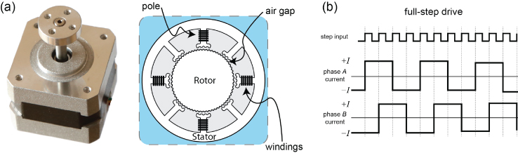
Figure 9-6: (a) Stepper motor external and internal structure; (b) full- and half-step drive signals
The EasyDriver Stepper Motor Driver
An easy way to generate the stepper motor pulse signals is to use a stepper-motor driver board. The EasyDriver board (illustrated in Figure 9-7) is a low-cost (~$15) open-hardware stepper motor driver board that is widely available. It can be used to drive four-, six-, and eight-wire stepper motors. The board has an output drive capability of between 7 V and 30 V at ±750 mA per phase. The board uses the Allegro A3967 Microstepping Driver with Translator, which allows for full, half, quarter, and one-eighth step microstepping modes. In addition, the board can be driven with 5 V or 3.3 V logic levels, which makes it an ideal board for use with the Beagle boards. For 3.3 V logic control levels, there is a jumper (SJ2) that has to be solder bridged.

Figure 9-7: Driving a stepper motor using the open-hardware EasyDriver board
The merit in examining this board is that many boards can be used for higher-powered stepper motors that have a similar design.
A Beagle Board Stepper Motor Driver Circuit
The EasyDriver board can be connected to the PocketBeagle as illustrated in Figure 9-8, using GPIOs for each of the control signals. The pins on the EasyDriver board are described in Figure 9-7, and a table is provided in the figure for the MS1/MS2 inputs. A C++ class called StepperMotor is available that accepts alternative GPIO numbers.
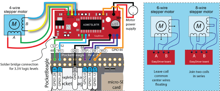
Figure 9-8: Driving a stepper motor using the PocketBeagle and the EasyDriver interface board
Controlling a Stepper Motor Using C++
Listing 9-3 presents the description of a class that can be used to control the EasyDriver board using five PocketBeagle GPIO pins. This code can be adapted to drive most types of stepper driver boards from any Beagle board.
Listing 9-3: /library/motor/StepperMotor.h (Segment)
class StepperMotor {public:enum STEP_MODE { STEP_FULL, STEP_HALF, STEP_QUARTER, STEP_EIGHT };enum DIRECTION { CLOCKWISE, ANTICLOCKWISE };private:// The GPIO pins MS1, MS2 (Microstepping options), STEP (The low->high step)// SLP (Sleep - active low) and DIR (Direction)GPIO *gpio_MS1, *gpio_MS2, *gpio_STEP, *gpio_SLP, *gpio_DIR;…public:StepperMotor(GPIO *gpio_MS1, GPIO *gpio_MS2, GPIO *gpio_STEP, GPIO *gpio_SLP,GPIO *gpio_DIR, int speedRPM = 60, int stepsPerRevolution = 200);StepperMotor(int gpio_MS1, int gpio_MS2, int gpio_STEP, int gpio_SLP,int gpio_DIR, int speedRPM = 60, int stepsPerRevolution = 200);virtual void step();virtual void step(int numberOfSteps);virtual int threadedStepForDuration(int numberOfSteps, int duration_ms);virtual void threadedStepCancel() { this->threadRunning = false; }virtual void rotate(float degrees);virtual void setDirection(DIRECTION direction);virtual DIRECTION getDirection() { return this->direction; }virtual void reverseDirection();virtual void setStepMode(STEP_MODE mode);virtual STEP_MODE getStepMode() { return stepMode; }virtual void setSpeed(float rpm);virtual float getSpeed() { return speed; }virtual void setStepsPerRevolution(int steps) { stepsPerRevolution = steps; }virtual int getStepsPerRevolution() { return stepsPerRevolution; }virtual void sleep();virtual void wake();virtual bool isAsleep() { return asleep; }virtual ~StepperMotor();… //Full code available in /library/motor/StepperMotor.h};
The library code is used in Listing 9-4 to create a StepperMotor object and rotate the motor counterclockwise 10 times at full-step resolution. It then uses a threaded step function to microstep the stepper motor clockwise for one full revolution over five seconds at one-eighth step resolution.
Listing 9-4: /chp09/stepper/StepperMotorApp.cpp
#include <iostream>#include <unistd.h>#include "motor/StepperMotor.h"using namespace std;using namespace exploringBB;int main(){cout << "Starting EBB Stepper Motor Example:" << endl;//Using 5 GPIOs, RPM=60 and 200 steps per revolution//MS1=52, MS2=44, STEP=64, SLP=60, DIR=46StepperMotor m(52,44,64,60,46,60,200);m.setDirection(StepperMotor::ANTICLOCKWISE);m.setStepMode(StepperMotor::STEP_FULL);m.setSpeed(100); //rpmcout << "Rotating 10 times at 100 rpm anti-clockwise, full step…" << endl;m.rotate(3600.0f); //in degreescout << "Finished regular (non-threaded) rotation)" << endl;m.setDirection(StepperMotor::CLOCKWISE);cout << "Performing 1 threaded revolution in 5 seconds using micro-stepping:" << endl;m.setStepMode(StepperMotor::STEP_EIGHT);if(m.threadedStepForDuration(1600, 5000)<0){cout << "Failed to start the Stepper Thread" << endl;}cout << "Thread should now be running…" << endl;for(int i=0; i<10; i++){ // sleep for 10 seconds.usleep(1000000);cout << i+1 << " seconds has passed…" << endl;}m.sleep(); // cut power to the stepper motorcout << "End of Stepper Motor Example" << endl;}
After calling the associated build script, the program can be executed and should result in the following output:
debian@ebb:~/exploringbb/chp09/stepper$ ./StepperAppStarting EBB Stepper Motor Example:Rotating 10 times at 100 rpm anti-clockwise, full step…Finished regular (non-threaded) rotation)Performing 1 threaded revolution in 5 seconds using micro-stepping:Thread should now be running…1 seconds has passed…2 seconds has passed……10 seconds has passed…End of Stepper Motor Example
It is important to note that the threaded revolution completes the revolution after five seconds. The counter continues for a further five seconds, during which time a holding torque is applied. The final call to m.sleep() removes power from the stepper motor coils, thus removing holding torque.
It is possible to further reduce the number of pins that are used in this motor controller example by using 74HC595 ICs and the SPI bus, as described in Chapter 8.
Relays
Traditional relays are electromechanical switches that are typically used to control a high-voltage/high-current signal using a low-voltage/low-current signal. They are constructed to enable a low-powered circuit to apply a magnetic force to an internal movable switch. The internal switch can turn on or turn off a second circuit that often contains a high-powered DC or AC load. The relay itself is chosen according to the power requirements; whether the circuit is designed so that the high-powered circuit is normally powered or normally disabled; and the number of circuits being switched in parallel.
Electromechanical relays (EMRs) are prone to switch bounce and mechanical fatigue, so they have a limited life span, particularly if they are switched constantly at frequencies of more than a few times per minute. Rapid switching of EMRs can also cause them to overheat. More recent, solid-state relays (SSRs) are electronic switches that consist of FETs, thyristors, and opto-couplers. They have no moving parts and therefore have longer life spans and higher maximum switching frequencies (about 1 kHz). The downside is that SSRs are more expensive, and they are prone to failure (often in the switched “on” state) because of overloading or improper wiring. They are typically installed with heat sinks and fast-blow fuses on the load circuit.
EMRs and SSRs are available that can switch high currents and voltages. That makes them particularly useful for applications such as smart home installations, the control of mains-powered devices, motor vehicle applications for switching high-current DC loads, and powering high-current inductive loads in robotic applications. Importantly, wiring mains applications is for expert users only, as even low currents coupled with high voltages can be fatal. Please seek local professional advice if dealing in any way with high currents or high voltages, including, but not limited to, AC mains voltages.
Figure 9-9(a) illustrates the type of circuit that can be used to interface the PocketBeagle to a relay. It is important that the relay chosen is capable of being switched at 5 V and that, like the motor circuit in Figure 9-3, a flyback diode is placed in parallel to the relay's inductive load to protect the FET from damage. Pololu (www.pololu.com) sells a small SPDT relay kit (~$4), as illustrated in Figure 9-9(b), that can be used to switch 8 A currents at 30 V DC using an Omron G5LE power relay. The breakout board contains a BSS138 FET, the flyback diode, and LEDs that indicate when the relay is switched to enable—that is, close the circuit connected to the normally open (NO) output.
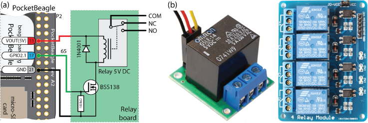
Figure 9-9: (a) Controlling a relay using the PocketBeagle; (b) example relay breakout boards
The relay can be connected to a regular GPIO for control. For example, if the relay were connected as shown in Figure 9-9(a) to P2.17 (GPIO2.1), which is GPIO 65, then it can be switched using the following:
debian@ebb:/sys/class/gpio/gpio65$ echo out > directiondebian@ebb:/sys/class/gpio/gpio65$ cat value0debian@ebb:/sys/class/gpio/gpio65$ echo 1 > valuedebian@ebb:/sys/class/gpio/gpio65$ echo 0 > value
Interfacing to Analog Sensors
A transducer is a device that converts variations in one form of energy into proportional variations in another form of energy. For example, a microphone is an acoustic transducer that converts variations in sound waves into proportional variations in an electrical signal. In fact, actuators are also transducers, as they convert electrical energy into mechanical energy.
Transducers, the main role of which is to convert information about the physical environment into electrical signals (voltages or currents), are called sensors. Sensors may contain additional circuitry to further condition the electrical signal (e.g., by filtering out noise or averaging values over time), and this combination is often referred to as an instrument. The terms sensor, transducer, and instrument are in fact often used interchangeably, so too much should not be read into the distinctions between them. Interfacing to sensors enables you to build an incredibly versatile range of project types using the Beagle boards, some of which are described in Table 9-2.
Table 9-2: Example Analog Sensor Types and Applications
| MEASURE | APPLICATIONS | EXAMPLE SENSORS |
| Temperature | Smart home, weather monitoring. | TMP36 temperature sensor. MAX6605 low-power temperature sensor. |
| Light Level | Home automation, display contrast adjustment. | Mini photocell/photodetector (PDV-P8001). |
| Distance | Robotic navigation, reversing sensing. | Sharp infrared proximity sensors (e.g., GP2D12). |
| Touch | User interfaces, proximity detection. | Capacitive touch. The AM335x ADC has touchscreen functionality. |
| Acceleration | Determine orientation, impact detection. | Accelerometer (ADXL335). Gyroscope (LPR530) detects change in orientation. |
| Sound | Speech recording and recognition, UV meters. | Electret microphone (MAX9814), MEMS microphone (ADMP401). |
| Magnetic Fields | Noncontact current measurement, home security, noncontact switches. | 100 A Non-invasive current sensor (SCT-013-000). Hall effect and reed switches. Linear magnetic field sensor (AD22151). |
| Motion Detection | Home security, wildlife photography. | PIR Motion Sensor (SE-10). |
The ADXL345 I2C/SPI digital accelerometer is discussed in Chapter 8, and Table 9-2 identifies another accelerometer, the ADXL335, which is an analog accelerometer. Essentially, the ADXL345 digital accelerometer is an analog sensor that also contains filtering circuitry, analog-to-digital conversion, and input/output circuitry. It is quite often the case that both analog and digital sensors are available that can perform similar tasks. Table 9-3 provides a summary comparison of digital versus analog sensors.
Table 9-3: Comparison of Typical Digital and Analog Sensor Devices
| DIGITAL SENSORS | ANALOG SENSORS |
| ADC is handled by the sensor, freeing up limited microcontroller ADC inputs. | Provide continuous voltage output and capability for fast sampling rates. |
| The real-time issues surrounding embedded Linux, such as variable sampling periods, are not as significant. | Typically less expensive but may require external components to configure the sensor parameters. |
| Often contain advanced filters that can be configured and controlled via registers. | Output is generally easy to understand without the need for complex datasheets. |
| Bus interfaces allow for the connection of many sensor devices. | Relatively easy to interface. |
| Less susceptible to noise. |
Digital sensors typically have more advanced features (e.g., the ADXL345 has double-tap and free-fall detection), but at a greater cost and level of complexity. Many sensors are not available in a digital package, so it is important to understand how to connect analog sensors to your Beagle board. Ideally, the analog sensor that you connect should not have to be sampled at a rate of thousands of times per second, or it will add significant CPU overhead.
Protecting the ADC Inputs
The Beagle board ADC is easily damaged as it is primarily intended to be a touchscreen controller for the AM335x, rather than a general-purpose ADC. In addition, many of the analog sensors that are described in Table 9-2 require 3.3 V or 5 V supplies. This is a particular concern when prototyping a new sensor interface circuit, as one connection mistake could physically damage the board. The ADC inputs do have some internal circuitry for protection, but it is not designed to carry even a modest current for more than short periods of time. The internal circuitry is mainly present for electrostatic discharge (ESD) protection, rather than to be relied on for clamping input signals. Therefore, external circuit protection is useful in preventing damage.
Diode Clamping
Figure 9-10(a) illustrates a simple diode clamping circuit that is typically used to limit voltage levels applied to ADCs. The circuit consists of two diodes and a current limiting resistor. The diodes are reverse biased when the voltage level is within the range 0 V to Vref. Current flows to the notional AIN0 input, and the circuit behaves correctly as illustrated in Figure 9-10(b) when a sine wave is applied (VIN ) that oscillates within the 0 V to Vref range. However, if VIN exceeds the Vref level (plus the forward voltage drop of the diode), then the upper diode is forward biased and current would flow to the Vref rail. If Vref is 1.8 V and silicon diodes are used (~0.7 V forward voltage), then this signal will be clamped at 2.5 V. For the lower diode, if VIN falls below 0 V–0.7 V, then the diode will be forward biased and AGND will source current. The resistor R can be used to limit the upper current level. The resulting clamped output is illustrated in Figure 9-10(c) when a sine wave is applied to the input that exceeds the permitted range.
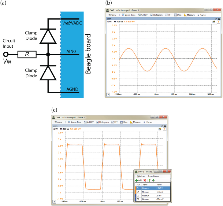
Figure 9-10: A typical diode clamping circuit (not recommended)
The clamping circuit in Figure 9-10(a) is not recommended for use with the AM335x for two reasons. First, the forward voltage drop of a typical silicon diode extends the nonclamped range to approximately -0.7 V to 2.5 V, which is well outside acceptable levels. More expensive Schottky diodes can be used that have a forward voltage drop of about 0.25 V at 2 mA and 25°C (e.g., the 1N5817G). These would bring the effective output range to about -0.25 V to 2.05 V, which is better but still not ideal. The second reason is that when clamping occurs, the current would need to be sourced from or sinked to the Beagle board's AGND or Vref rails. Sinking current to the Vref rail could damage the Vref input and/or affect the reference voltage level. However, diode clamping is preferable to no protection whatsoever.
Op-Amp Clamping
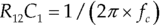
A recommended circuit to protect the ADC circuitry is presented in Figure 9-11(a). While it appears complex, it is reasonably easy to connect, as it requires only three ICs and seven resistors to protect all seven or eight AINs. This voltage follower circuit uses a 5 V powered single op-amp package to provide a 1.8 V voltage reference source to an array of low-voltage op-amps. The Microchip MCP6001/2 or LM358 can be used for this voltage supply task.
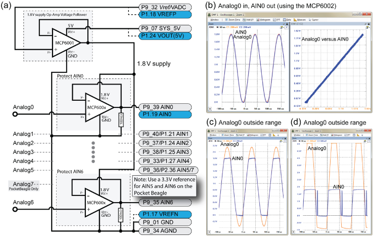
Figure 9-11: Protecting the ADC inputs using 1.8 V powered op-amps (recommended); (a) the circuit to protect all analog inputs on the BeagleBone and PocketBeagle boards; (b) linear response characteristic; (c) clipped response to an out-of-range input; and (d) clipped response to a significantly out-of-range input
An array of modern op-amps, supplied at 1.8 V (i.e., VCC+ = 1.8 V), are configured in voltage follower configuration and placed in front of each of the ADC inputs AIN0 to AIN6/7. You can use a 3.3 V reference voltage for the AIN5 and AIN6 inputs on the PocketBeagle.
These op-amps are supplied with VDD = VCC+ = 1.8 V and VSS = VCC- = GND, so it is not possible for their output voltage levels to exceed the range 0 V to 1.8 V. The MCP600x is a low-cost DIP packaged op-amp that is suitable for this role. In particular, the MCP6004 has four op-amps within the one package, so only two MCP6004s (plus the 1.8 V supply circuit op-amp) are required to protect all seven/eight ADC inputs.
Figure 9-11(b) illustrates the behavior of this circuit when a 0.9 V amplitude sine wave (biased at +0.9 V) is applied to the Analog0 circuit input. The output signal overlays precisely on the input signal. Older op-amps (including the LM358) would have difficulty with this type of rail-to-rail operation (i.e., 0 V to 1.8 V) and would behave in a nonlinear way near the rail voltages. As shown in the plot of the Analog0 input versus the AIN0 output in Figure 9-11(b), there is a strong linear relationship, even at the supply rail voltage levels. Figure 9-11(c) and (d) illustrate the consequence of the input signal (accidently) exceeding the allowable range. In both cases the output is clamped to the 0 V to 1.8 V range and the AM335x ADC is protected, though (of course) the signal input to the ADC is distorted.
The circuit can be connected to the Beagle board as illustrated in Figure 9-11(a), and its impact can be evaluated in a terminal using the following steps (e.g., on the PocketBeagle):
debian@ebb:~$ cd /sys/bus/iio/devices/iio:device0debian@ebb:/sys/bus/iio/devices/iio:device0$ lsbuffer in_voltage2_raw in_voltage6_raw powerdev in_voltage3_raw in_voltage7_raw scan_elementsin_voltage0_raw in_voltage4_raw name subsystemin_voltage1_raw in_voltage5_raw of_node uevent
Setting the DC voltage levels at Analog0 (P1.19) to be 0 V (P1.19 connected to P1.17 VREFN), 0.9 V, 1.8 V, and 2.1 V results in the respective raw input values from the 12-bit ADC (0-4095) as follows:
debian@ebb:/sys/bus/iio/devices/iio:device0$ cat in_voltage0_raw0debian@ebb:/sys/bus/iio/devices/iio:device0$ cat in_voltage0_raw2107debian@ebb:/sys/bus/iio/devices/iio:device0$ cat in_voltage0_raw4026debian@ebb:/sys/bus/iio/devices/iio:device0$ cat in_voltage0_raw4024
The 100 kΩ resistor ensures that current flows to GND through the resistor rather than through the AINx input. (For your reference, the Touchscreen Controller ADC functional block diagram is shown in Figure 12-2 of the AM335x TRM.) The AM335x datasheet at tiny.cc/beagle903 provides further details about the limitations of the AM335x ADC.
Analog Sensor Signal Conditioning
One of the problems with analog sensors is that they may have output signal voltage levels quite different from those required by the AM335x ADC. For example, the Sharp GP2D12 distance sensor that is used as an example in this section outputs a DC voltage of ~2.6 V when it detects an object at a distance of 10 cm and of ~0.4 V when the object is detected at a distance of 80 cm. If this sensor is connected to the clamping circuit in Figure 9-11(a), the AM335x ADC would not be damaged, but the sensing distance range would be reduced by clamping.
Signal conditioning is the term used to describe the manipulation of an analog signal so that it is suitable for the next stage of processing. To condition a sensor output as an input to the Beagle boards, this often means ensuring that the signal's range is less than 1.8 V, with a DC bias of +0.9 V.
Scaling Using Voltage Division
The voltage divider circuit described at the beginning of Chapter 4 can be used to condition a sensor output. If the output voltage from the sensor is greater than 1.8 V but not less than 0 V, then a voltage divider circuit can be used to linearly reduce the voltage to remain within a 0 V–1.8 V range.
Figure 9-13 illustrates a voltage division circuit and its integration with the 1.8 V op-amp protection circuitry discussed in the previous section. Voltage follower circuits also act as buffer circuits. The maximum input impedance of the AM335x ADC inputs ranges from about 76 kΩ at the highest frequencies to many megaohms at low frequencies.3 The voltage divider circuit will further load the sensor output impedance (perhaps requiring further unity-gain buffers before the voltage divider). However, the MCP6002 will act as a buffer that prevents the sensor circuit from exceeding the maximum input impedance of the ADC (remember that ideal voltage follower circuits have infinite input impedance and zero output impedance). There are some important points to note about this circuit:
- Resistors have a manufacturing tolerance (often 5%–10% of the resistance value), which will affect the scaling accuracy of the voltage division circuit. You may need to experiment with combinations or use a potentiometer to adjust the resistance ratio.
- A capacitor C1 can be added across VOUT
to reduce noise if required. The value of C1 can be chosen according to the value of R1 and the desired cutoff frequency fC, according to the equation
 , where
  . (i.e., R1 in parallel with R2). There is an example in the next section.
 - With multi-op-amp packages, unused inputs should be connected as shown in Figure 9-13 (in light gray) to avoid random switching noise.
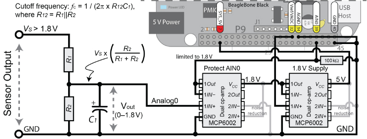
Figure 9-13: Scaling an input signal using voltage division with op-amp ADC protection in place
This circuit works well for linearly scaling down an input signal, but it would not work for a zero-centered or negatively biased input signal. For that, a more general and slightly more complex op-amp circuit is required.
Signal Offsetting and Scaling
Figure 9-14(a) provides a general op-amp circuit that can be used to set the gain and offset of an input signal. Do not connect this circuit directly to the Beagle board—it is designed as an adjustable prototyping circuit to use in conjunction with an oscilloscope to design a fixed-signal conditioning circuit for your particular application. Some notes on this circuit:
- The Vcc- input of the op-amp is tied to GND, which is representative of the type of circuit that is built using the Beagle boards, as a –5 V rail is not readily available.
- If an LM358 is used, then a load resistor is required to prevent the output from being clamped below 0.7 V. According to the National Semiconductor Corporation (1994), “the LM358 output voltage needs to raise approximately one diode drop above ground to bias the on-chip vertical PNP transistor for output current sinking applications.”
- The 1.8 V level can be provided by the analog voltage reference on the Beagle boards, but do not connect it without the use of a voltage follower circuit as shown earlier. Alternatively, a voltage divider could be used with the 5 V rail.
- A 100 nF decoupling capacitor can be used on the VIN input to remove the DC component of the incoming sensor signal. However, for many sensor circuits, the DC component of the sensor signal is important and should not be removed.
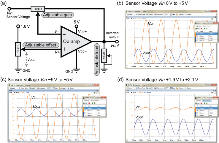
Figure 9-14: (a) A general op-amp signal conditioning circuit that inverts the input; (b) conditioned output when Vin is 0 V to 5 V; (c) output when Vin is −5 V to +5 V; (d) conditioned and amplified output when the input signal is 1.9 V to 2.1 V
The circuit in Figure 9-14(a) amplifies (or attenuates), offsets, and inverts the input signal according to the settings of the potentiometers:
- The gain is set using the adjustable gain potentiometer, where
 .
. - The offset is set using the adjustable offset potentiometer. This can be used to center the output signal at 0.9 V.
- The output voltage is approximately
 . As such, the output is an inverted and scaled version of the input signal.
 - The inversion of the signal (you can see that the output is at a maximum when the input is at a minimum) is a consequence of the circuit used. Non-inverting circuits are possible but they are more difficult to configure. The inversion can easily be corrected in software by subtracting the received ADC input value from 4,095.
In Figure 9-14(b), (c), and (d) the offset voltage is set to 0.9 V, and the gain is adjusted to maximize the output signal (between 0 and 1.8 V) without clipping the signal. In Figure 9-14(b), the gain and offset are adjusted to map a 0 V to +5 V signal to a 1.8 V to 0 V inverted output signal. In Figure 9-14(c), a –5 V to +5 V signal is mapped to a 1.8 V to 0 V signal. Finally, in Figure 9-14 (d), a 1.9 V to 2.1 V input signal is mapped to a 1.3 V to 0 V output (this is the limit for the LM358 in this case). The last case is applied to an example application in the next section.
Figure 9-15 illustrates a full implementation of the op-amp signal conditioning circuit as it is attached to the BeagleBone board. In this example, only two op-amps are required in total. This is because the MCP6002 on the left is used to both condition the signal and protect the ADC input. This is possible because it is powered using a VCC = 1.8 V supply, which is provided by the 1.8 V voltage follower circuit on the right side. The MCP6002 is a dual op-amp package, and it is used because the MCP6001 is not readily available in a DIP package. You could use the MCP6002 to condition two separate sensor signals.

Figure 9-15: Signal conditioning circuit connected to the BBB with gain set using R1 and R2 and offset set using R3 and R4
The potentiometers in Figure 9-14 are replaced by fixed-value resistors in Figure 9-15 to demonstrate how a fixed offset and gain can be configured. In addition, the MCP6002 does not require a load resistor on the output, but a 100 kΩ resistor is used to protect the ADC input.
If the input voltage is –5 V to +5 V, then this circuit will give an output of 0.048 V to 1.626 V with the resistor values R1 = 9.1 kΩ, R2 = 1.5 kΩ, R3 = 4.7 kΩ, and R4 = 6.5 kΩ. A general equation to describe the relationship between the input and output can be determined as follows:
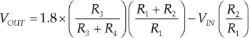
At VIN = 5 V, VOUT = –0.05 V, and at VIN = –5 V, VOUT = 1.71 V.
Listing 9-5 displays a test program that can be used to read in 1,000 values from AIN0 at about 20 Hz, with the output presented on a single line.
Listing 9-5: /exploringbb/chp09/testADC/testADC.cpp (Segment)
#define LDR_PATH "/sys/bus/iio/devices/iio:device0/in_voltage"int readAnalog(int number){stringstream ss;ss << LDR_PATH << number << "_raw";fstream fs;fs.open(ss.str().c_str(), fstream::in);fs >> number;fs.close();return number;}int main(int argc, char* argv[]){cout << "The value on the ADC is:" << endl;for(int i=0; i<1000; i++){int value = readAnalog(0);cout << " = " << readAnalog(0) << "/4095 " << ' ' << flush;usleep(50000);}return 0;}
When built and executed, this code gives the following output:
debian@ebb:~/exploringbb/chp09/testADC$ ./builddebian@ebb:~/exploringbb/chp09/testADC$ ./testADCThe value on the ADC is: = 2140/4095
If a sine wave is inputted at a frequency of 0.1 Hz, then the output of the program will slowly increase and decrease between a value close to 0 and a value close to 4,095.
Analog Interfacing Examples
Now that the Beagle board's ADC inputs can be protected from damage using op-amp clamping, two analog interfacing examples are discussed in this section. The first example demonstrates how you can model the response of a sensor, and the second example employs signal offsetting and scaling.
Infrared Distance Sensing
Sharp infrared (IR) distance measurement sensors are useful for robotic navigation applications (e.g., object detection and line following) and proximity switches (e.g., automatic faucets and energy-saving switches). These sensors can also be attached to servo motors and used to calculate range maps (e.g., on the front of a mobile robot). They work well in indoor environments but have limited use in direct sunlight. They have a response time of ~39 ms, so at 25–26 readings per second they will not provide dense range images. Figure 9-16(a) shows two aspect views of a low-cost sensor, the Sharp GP2D12.

Figure 9-16: (a) Sharp infrared distance measurement sensor; (b) its analog output response
This is a good analog sensor integration example because four problems need to be resolved, which occur generally with other sensors.
- The sensor response in Figure 9-16(b) is highly nonlinear so that two different distances can give the same sensor output. Thus, you need to find a way to disambiguate the sensor output. For example, if the sensor output is 1.5 V, it could mean that the detected object is either 5 cm or 17 cm from the sensor. A common solution to this problem is to mount the sensor so that it is physically impossible for an object to be closer than 10 cm from the sensor. This problem is not examined in further detail, and it is assumed here that the detected object cannot be closer than 10 cm from the sensor.
- The voltage value (0 V to 2.6 V) exceeds the ADC range. As shown, a signal conditioning circuit can be designed to solve this problem.
- The output signal is prone to high-frequency noise. A low-pass RC filter can be designed to solve this problem.
- Even for the assumed distances of 10 cm or greater, the relationship between distance and voltage output is still nonlinear. A curve-fitting process can be employed to solve this problem if a linear relationship is required (e.g., threshold applications do not require a linear relationship—just a set value).
To solve the second problem, a voltage divider configuration can be employed to map the output voltage range from 0 V–2.6 V to 0 V –1.8 V. A 10 kΩ potentiometer can be used for this task, as shown in Figure 9-17(a), where 69.2 percent (100 × 1.8 V/2.6 V) of the voltage needs to be dropped across the lower resistor. Therefore, if the total resistance is 10 kΩ, then the lower resistor would be 6.92 kΩ. If fixed-value resistors are to permanently replace the adjustable potentiometer, then 6.8 kΩ and 3.3 kΩ could be used. Accuracy is not vital, as the op-amp circuit protects the ADC input and the sensor is itself separately calibrated based on the actual resistor values used.
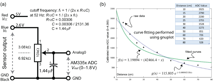
Figure 9-17: (a) A voltage divider circuit configured for the GP2D12 sensor; (b) the plot of the fitting data from gnuplot
To solve the third problem, the circuit in Figure 9-17(a) includes a low-pass RC filter to remove high-frequency signal noise. The last step determined the series resistor to be approximately 3.3 kΩ; therefore, a capacitor value must be chosen to suit the cutoff sampling frequency, which is about 52 Hz (i.e., 2 × 26 Hz) in this case (taking account of the Nyquist criterion). A capacitor value of 1 μF provides an appropriate value, given the equation ![]() .
.
To solve the final problem, a small test rig can be set up to calibrate the distance sensor. A measuring tape can be placed at the front of the sensor, and a large object can be positioned at varying distances from the sensor, between 10 cm and 80 cm. In my case, this provided the raw data for the table in Figure 9-17(b), which is plotted on the graph with the square markers.
This raw data is not sufficiently fine to determine the distance value represented by an ADC measurement intermediate between the values corresponding to the squares. Therefore, curve fitting can be employed to provide an expression that can be implemented in program code. The data can be supplied to the curve fitting tools that are freely available on the Wolfram Alpha website at www.wolframalpha.com. Using the following command string:
exponential fit {{3925,10}, {2790,15}, {2200,20}, {1755,25}, {1528,30},{1273,40}, {851,50}, {726,60}, {620,70}, {528,80}}
results in the expression ![]() (see
(see tiny.cc/beagle906). This curve is plotted in Figure 9-17(b) with the triangular markers. It could also be modeled with a quadratic using the following command string:
quadratic fit {{3925,10}, {2790,15}, {2200,20}, {1755,25}, {1528,30},{1273,40}, {851,50}, {726,60}, {620,70}, {528,80}}
which results in the expression ![]() (see
(see tiny.cc/ebb907).
Note that this process can be used for many analog sensor types to provide an expression that can be used to interpolate between the measured sensor values. What type of fitting curve best fits the data will vary according to the underlying physical process of the sensor. For example, you could use the linear fit command on the Wolfram Alpha website to derive an expression for the LDR described in Chapter 6. A C++ code example can be written to read in the ADC value and convert it into a distance, as shown in Listing 9-6, where the exponential fix expression is coded on a single line.
Listing 9-6: /exploringbb/chp09/IRdistance/IRdistance.cpp (Segment)
…int main(int argc, char* argv[]){cout << "Starting the IR distance sensor program:" << endl;for(int i=0; i<1000; i++){int value = readAnalog(0);float distance = 115.804f * exp(-0.000843107f * (float)value);cout << "The distance is: " << distance << " cm" << ' ' << flush;usleep(100000);}return 0;}
When the code example is executed, it continues to output the distance of a detected object in centimeters, for about 100 seconds.
debian@ebb:~/exploringbb/chp09/IRdistance$ ./builddebian@ebb:~/exploringbb/chp09/IRdistance$ ./IRdistanceStarting the IR distance sensor program:The distance is: 17.7579 cm
If the speed of execution of such code is vital in the application, then it is preferable to populate a lookup table (LUT) with the converted values. This means that each value is calculated once, either at the initialization stage of the program, or perhaps during code development, rather than every time a reading is made and has to be converted. When the program is in use, the subsequent memory accesses (for reading the LUT) are much more efficient than the corresponding floating-point calculations. This is possible because a 12-bit ADC can output only 4,096 unique values, and it is not unreasonable to store an array of the 4,096 possible outcomes in the memory associated with the program.
ADXL335 Conditioning Example
The ADXL335 is a small three-axis accelerometer that outputs an analog signal that has undergone conditioning. It behaves just like the ADXL345 except that the output is from three analog pins, one for each axis.
When measuring in a range of ±1g, the x-axis outputs ~1.30 V at 0°, ~1.64 V at 90°, and ~1.98 V at 180°. This means that the output signal of the breakout board is centered on 1.64 V and has a variation of ±0.34 V. A circuit can be designed as shown in Figure 9-18 to map the center point to 0.9 V and to extend the variation over the full 1.8 V range.
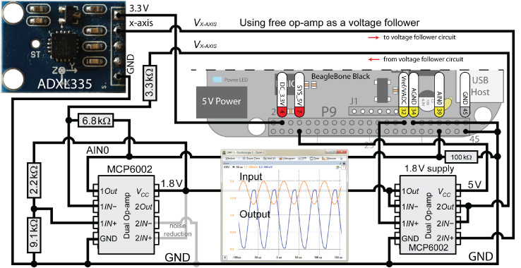
Figure 9-18: The ADXL335 analog accelerometer and its connection to the BBB with further signal conditioning
Unfortunately, there are output impedance problems with this particular ADXL335 breakout board, and the voltage divider circuit in the conditioning circuit will not function correctly. A buffer circuit is therefore required, and an op-amp in voltage follower configuration can be used. The 1.8 V powered op-amp could not be used for this task, as the upper sensor output (at 1.98 V) exceeds the 1.8 V output limit of that op-amp and would thus have been clamped. The 1.8 V supply op-amp IC on the right side has a limit of 5 V, so it is used for this task.
This circuit is a little complex, and it may be overkill, as the amplification of a signal does not necessarily improve the information content of that signal—noise is amplified along with the signal. It is quite possible that the 12-bit ADC performs just as well over a linearly scaled 1.3 V to 1.98 V range as it does over the full 0 V–1.8 V range for this particular sensor. However, it is important that you are exposed to the process of offsetting and scaling a signal using op-amps, as it is required for many sensor types, particularly those that are centered on 0 V, such as microphone audio signals.
The testADC program that was used previously can be used to print out the digitized AIN value from the accelerometer. In this case, the program prints out
debia@ebb:~/exploringbb/chp09/testADC$ ./testADCThe value on the ADC is: = 2174/4095
at rest (90°), 250 at 0°, and 4,083 at +180°. A simple linear interpolation can be used to approximate the intermediate values.
Interfacing to Local Displays
As described in Chapter 1, many Beagle boards can be attached to computer monitors and digital televisions using the HDMI output connector. In addition, LCD Capes and SPI LCD displays can be connected to the expansion headers. The downsides of such displays are that they may not be practical, or they may be overly expensive for certain applications. When a small amount of information needs to be relayed to a user, a simple LED can be used; for example, the onboard power and activity LEDs are useful indicators that the board continues to function. For more complex information, two possibilities are to interface to low-cost LED displays and low-cost character LCD modules.
In Chapter 8, an example is provided for driving seven-segment displays using SPI and 74HC595 serial shift register ICs. That is a useful educational exercise, but the wiring can quickly become impractical for multiple digits. In the following sections more advanced solutions are described for adding low-cost onboard display to your board.
MAX7219 Display Modules
The Maxim Integrated MAX7219 is a serially interfaced eight-digit LED display driver that is widely available and built in to low-cost multi-seven-segment display modules. The module in Figure 9-19(a) ($2–$3) is a 5 V eight-digit red LED display that contains the MAX7219 IC, which can be interfaced using SPI. The datasheet for the IC is available at tiny.cc/beagle908.
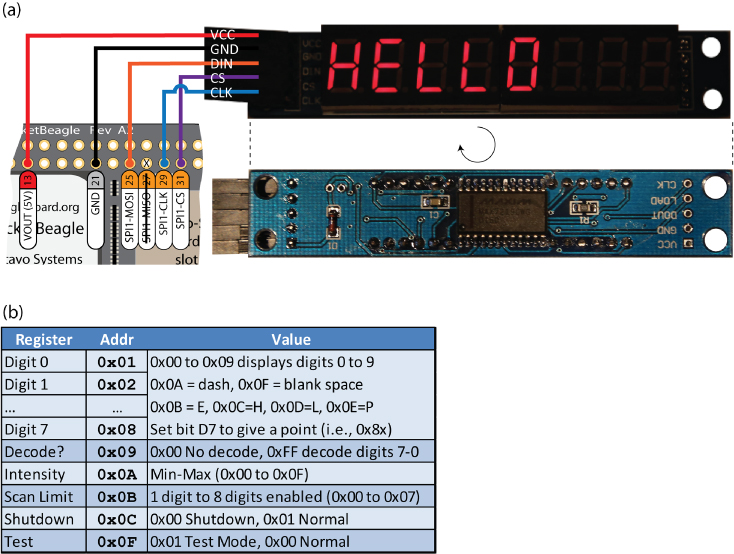
Figure 9-19: (a) The MAX7219 eight-digit seven-segment display module connected to the SPI1 bus on a PocketBeagle, and (b) a summary register table for the MAX7219
The module can be connected to the PocketBeagle using an SPI bus, which in this case is the SPI1 bus, as illustrated in Figure 9-19(a). Note that the module is powered using the 5V line but is controlled using 3.3V logic levels. Do not connect the DOUT line on the module directly back to the PocketBeagle SPI1-MISO input as you may damage your board!
In decode mode, the module can display eight digits consisting of the numeric values 0–9 (with a point), the letters H, E, L, P, a space, and a dash. The decode mode can also be disabled, permitting each of the seven-segments to be controlled directly. For example, the following steps that use the summary list of registers in Figure 9-19(b) can be used to test that the module is configured correctly by sending pairs of bytes to the device—the register address and data value to write:
- Turn on the module and then place the module in test mode (i.e., all segments on).4
debian@ebb:/dev$ echo -ne "x0Cx01" > /dev/spidev1.1debian@ebb:/dev$ echo -ne "x0Fx01" > /dev/spidev1.1 - Take the module out of test mode (return to its previous state).
debian@ebb:/dev$ echo -ne "x0Fx00" > /dev/spidev1.1 - Change to eight-segment mode and display the number 6.5 using the last two digits (i.e., on the RHS).
debian@ebb:/dev$ echo -ne "x09xFF" > /dev/spidev1.1debian@ebb:/dev$ echo -ne "x01x05" > /dev/spidev1.1debian@ebb:/dev$ echo -ne "x02x86" > /dev/spidev1.1 - Display the word “Hello ” (i.e., with three trailing spaces), as in Figure 9-19(a).
debian@ebb:/dev$ echo -ne "x08x0C" > /dev/spidev1.1debian@ebb:/dev$ echo -ne "x07x0B" > /dev/spidev1.1debian@ebb:/dev$ echo -ne "x06x0D" > /dev/spidev1.1debian@ebb:/dev$ echo -ne "x05x0D" > /dev/spidev1.1debian@ebb:/dev$ echo -ne "x04x00" > /dev/spidev1.1debian@ebb:/dev$ echo -ne "x03x0F" > /dev/spidev1.1debian@ebb:/dev$ echo -ne "x02x0F" > /dev/spidev1.1debian@ebb:/dev$ echo -ne "x01x0F" > /dev/spidev1.1 - Adjust the LED intensity to its darkest and to its brightest.
debian@ebb:/dev$ echo -ne "x0Ax00" > /dev/spidev1.1debian@ebb:/dev$ echo -ne "x0Ax0F" > /dev/spidev1.1 - Turn off the module.
debian@ebb:/dev$ echo -ne "x0Cx00" > /dev/spidev0.1
The code in Listing 9-7 uses the SPIDevice class from Chapter 8 to create a high-speed counter. The display module is responsive at an SPI bus speed of 10 MHz, updating the display 1,000,000 times in approximately 18 seconds. The output of the program in Listing 9-7 is displayed in Figure 9-20. The display is counting quickly, so the blurred digits on the RHS are caused by the update speed of the count relative to the camera shutter speed, which was used to capture this photograph.
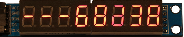
Figure 9-20: The MAX7219 eight-digit seven-segment display counting due to Listing 9-7 (photographed while counting)
Listing 9-7: chp09/max7219/max7219.cpp
#include <iostream>#include "bus/SPIDevice.h"using namespace exploringBB;using namespace std;int main(){cout << "Starting the MAX7219 example" << endl;SPIDevice *max = new SPIDevice(1,1);max->setSpeed(10000000); // max speed is 10MHzmax->setMode(SPIDevice::MODE0);// turn on the display and disable test mode -- just in case:max->writeRegister(0x0C, 0x01); // turn on the displaymax->writeRegister(0x0F, 0x00); // disable test modemax->writeRegister(0x0B, 0x07); // set 8-digit modemax->writeRegister(0x09, 0xFF); // set decode mode onfor(int i=1; i<9; i++){ // clear all digits to be dashesmax->writeRegister((unsigned int)i, 0x0A);}for(int i=0; i<=100000; i++){ // count to 100,000int val = i; // need to display each digitunsigned int place = 1; // the current decimal placewhile(val>0){ // repeatedly divide and get remaindermax->writeRegister( place++, (unsigned char) val%10);val = val/10;}}max->close();cout << "End of the MAX7219 example" << endl;return 0;}
Character LCD Modules
Character LCD modules are LCD dot matrix displays that feature pre-programmed font tables so that they can be used to display simple text messages without the need for complex display software. They are available in a range of character rows and columns (commonly 2×8, 2×16, 2×20, and 4×20) and usually contain an LED backlight, which is available in a range of colors. Recently, OLED (organic LED) versions and E-paper (e-ink) versions have been released that provide for greater levels of display contrast.
To understand the use of a character LCD module, you should study its datasheet. While most character LCD modules have common interfaces (often using a Hitachi HD44780 controller), the display modules from Newhaven have some of the best datasheets. The datasheet for a typical Newhaven display module is available at tiny.cc/beagle910. It is recommended that the datasheet be read in conjunction with this discussion. The datasheet for the HD44780 controller is available at tiny.cc/beagle911. The following code will work for all character LCD modules that are based on this controller.
There are character LCD modules available with integrated I2C and SPI interfaces, but the majority of modules are available with an eight-bit and four-bit parallel interface. By adding a 74HC595 to the circuit, it is possible to develop a custom SPI interface, which provides greater flexibility in the choice of modules. A generic character LCD module can be attached to the BBB using the wiring configuration illustrated in Figure 9-21.

Figure 9-21: SPI interfacing to character LCD modules using a 74HC595 8-bit serial shift register
You can interface to character LCD modules using either an eight-bit or a four-bit mode, but there is no difference in the functionality available with either mode. The four-bit interface requires fewer interface connections, but each eight-bit value has to be written in two steps—the lower four bits (nibble) followed by the higher four bits (nibble).
To write to the character LCD module two lines are required, the RS line (register select signal) and the E line (operational enable signal). The circuit in Figure 9-21 is designed to use a four-bit interface, as it requires only six lines rather than the 10 lines that would be required with the eight-bit interface. This means that a single eight-bit 74HC595 can be used to interface to the module when it is in four-bit mode. The downside is that the software is slightly more complex to write, as each byte must be written in two nibbles. The four-bit interface uses the inputs DB4–DB7, whereas the eight-bit interface requires the use of DB0–DB7.
It is possible to read data values from the display, but it is not required in this application; therefore, the R/W (read/write select signal) is tied to GND to place the display in write mode. The power is supplied using VCC (5 V) and VSS (GND). VEE sets the display contrast level and must be at a level between VSS and VCC. A 10 kΩ multi-turn potentiometer can be used to provide precise control over the display contrast. Finally, the LED+ and LED connections supply the LED backlight power.
The display character address codes are illustrated on the module in Figure 9-21. Using commands (on page 6 of the datasheet), data values can be sent to these addresses. For example, to display the letter A in the top-left corner, the following procedure can be used with the four-bit interface:
- Clear the display by sending the value 00000001 to D4–D7. This value should be sent in two parts: the lower nibble (0001), followed by the higher nibble (0000). The E line is set high and then low after each nibble is sent. A delay of 1.52 ms (datasheet, page 6) is required. The module expects a command to be sent when the RS line is low. After sending this command, the cursor is placed in the top-left corner.
- Write data 01000001 = 6510 = A (datasheet, page 9) with the lower nibble sent first, followed by the upper nibble. The E line is set high followed by low after each nibble is sent. The module expects data to be sent when the RS line is set high.
A C++ class is available for you to use in interfacing the Beagle boards to display modules using SPI. The class assumes that the 74HC595 lines are connected as shown in Figure 9-21, and the data is represented as in Table 9-5. The code does not use bits 2 (QD
) and 3 (QC
) on the 74HC595, so it is possible for you to repurpose these for your own application. For example, one pin could be connected to the gate of a FET and used to switch the backlight on and off. The class definition is provided in Listing 9-8, and the implementation is in the associated LCDCharacterDisplay.cpp file.
Table 9-5: Mapping of the 74HC595 Data Bits to the Character LCD Module Inputs, as Required for the C++ LCDCharacterDisplay Class
| BIT 7 MSB |
BIT 6 | BIT 5 | BIT 4 | BIT 3 | BIT 2 | BIT 1 | BIT 0 LSB |
|
| Character LCD module | D7 | D6 | D5 | D4 | Not used | Not used | E | RS |
| 74HC595 pins | QH | QG | QF | QE | QD | QC | QB | QA |
Listing 9-8: library/display/LCDCharacterDisplay.h
class LCDCharacterDisplay {private:SPIDevice *device;int width, height;…public:LCDCharacterDisplay(SPIDevice *device, int width, int height);virtual void write(char c);virtual void print(std::string message);virtual void clear();virtual void home();virtual int setCursorPosition(int row, int column);virtual void setDisplayOff(bool displayOff);virtual void setCursorOff(bool cursorOff);virtual void setCursorBlink(bool isBlink);virtual void setCursorMoveOff(bool cursorMoveOff);virtual void setCursorMoveLeft(bool cursorMoveLeft);virtual void setAutoscroll(bool isAutoscroll);virtual void setScrollDisplayLeft(bool scrollLeft);virtual ~LCDCharacterDisplay();};
The constructor requires an SPIDevice object and details about the width and height of the character display module (in characters). The constructor provides functionality to position the cursor on the display and to describe how the cursor should behave (e.g., blinking or moving to the left/right). This class can be used as shown in Listing 9-9 to create an LCDCharacterDisplay object, display a string, and display a count from 0 to 10,000 on the module.
Listing 9-9: chp09/LCDcharacter/LCDApp.cpp
#include <iostream>#include <sstream>#include "display/LCDCharacterDisplay.h"using namespace std;using namespace exploringBB;int main(){cout << "Starting EBB LCD Character Display Example" << endl;SPIDevice *busDevice = new SPIDevice(2,0); //Using second SPI bus (both loaded)busDevice->setSpeed(1000000); // Have access to SPI Device objectostringstream s; // Using this to combine text and int dataLCDCharacterDisplay display(busDevice, 16, 2); // Construct 16x2 LCD Displaydisplay.clear(); // Clear the character LCD moduledisplay.home(); // Move the cursor to the (0,0) positiondisplay.print("EBB by D. Molloy"); // String to display on the first rowfor(int x=0; x<=10000; x++){ // Do this 10,000 timess.str(""); // clear the ostringstream object sdisplay.setCursorPosition(1,3); // move the cursor to second rows << "X=" << x; // construct a string that has an int valuedisplay.print(s.str()); // print the string X=*** on the LCD module}cout << "End of EBB LCD Character Display Example" << endl;}
The code example in Listing 9-9 can be built and executed using the following steps:
debian@ebb:~/exploringbb/chp09/LCDcharacter$ ./builddebian@ebb:~/exploringbb/chp09/LCDcharacter$ ./LCDApp
The count incrementally updates on the display and finishes with the output illustrated in Figure 9-22.
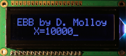
Figure 9-22: Output from Listing 9-9 on a Newhaven display module
It takes 26 seconds to display a count that runs from 0 to 10,000, which is approximately 385 localized screen updates per second. This means that you could potentially connect many display modules to a single SPI bus and still achieve reasonable screen refresh rates. You would require the type of multiple SPI slave circuitry that is discussed in Chapter 8, which would require ![]() GPIOs for x modules. At its maximum refresh rate, the
GPIOs for x modules. At its maximum refresh rate, the top command gives the following output:
PID USER PR NI VIRT RES SHR S %CPU %MEM TIME+ COMMAND18227 root 20 0 0 0 0 S 34.6 0.0 25:02.50 spi220967 debian 20 0 2708 988 856 S 33.9 0.2 0:04.15 LCDApp
This indicates that the LCDApp program and its associated spi2 platform device are utilizing 68.5 percent of the available CPU time at this extreme module display refresh rate of 385 updates per second. To be clear, the display maintains its current display state without any Linux overhead, and refresh is only required to change the display contents.
Building C/C++ Libraries
In this chapter, a number of different actuators, sensors, and display devices are interfaced to the Beagle boards using stand-alone code examples. Should you embark upon a grand design project, it will quickly become necessary to combine such code examples together into a single software project. In addition, it would not be ideal if you had to recompile every line of code in the project each time you made a change. To solve this problem, you can build your own libraries of C/C++ code, and to assist you in this task, you can use makefiles, and better still, CMake.
Makefiles
As the complexity of your C/C++ projects grows, an IDE such as Eclipse can be used to manage compiler options and program code interdependencies. However, there are occasions when command-line compilation is required; and when projects are complex, a structured approach to managing the build process is necessary. A good solution is to use the make program and makefiles.
The process is best explained by using an example. To compile a hello.cpp program and a test.cpp program within a single project without makefiles, the build script can be as follows:
debian@ebb:~/exploringbb/chp09/makefiles$ more build#!/bin/bashg++ -o3 hello.cpp -o hellog++ -o3 test.cpp -o test
The script works perfectly fine; however, if the project's complexity necessitated separate compilation, then this approach lacks structure. The following is a simple Makefile file that could be used instead (it is important to use the Tab key to indent the lines with the <Tab> marker shown here):
debian@ebb:~/exploringbb/chp09/makefiles$ more Makefileall: hello testhello:<Tab> g++ -o3 hello.cpp -o hellotest:<Tab> g++ -o3 test.cpp -o testdebian@ebb:~/exploringbb/chp09/makefiles$ rm hello testdebian@ebb:~/exploringbb/chp09/makefiles$ makeg++ -o3 hello.cpp -o hellog++ -o3 test.cpp -o test
If the make command is issued in this directory, the Makefile file is detected, and a call to make all will automatically be invoked. That will execute the commands under the hello: and test: labels, which build the two programs. However, this Makefile file does not add much in the way of structure, so a more complete version is required, such as this:
debian@ebb:~/exploringbb/chp09/makefiles2$ more MakefileCC = g++CFLAGS = -c -o3 -WallLDFLAGS =all: hello testhello: hello.o<tab> $(CC) $< -o $@hello.o: hello.cpp<tab> $(CC) $(CFLAGS) $< -o $@test: test.o<tab> $(CC) $(LDFLAGS) $< -o $@test.o: test.cpp<tab> $(CC) $(CFLAGS) $< -o $@clean:<tab> rm -rf *.o hello test
In this version, the compiler choice, compiler options, and linker options are defined at the top of the Makefile file. This enables the options to be easily altered for all files in the project. In addition, the object files (.o files) are retained, which dramatically reduces repeated compilation times when there are many source files in the project. There is some shortcut syntax in this Makefile file. For example, $< is the name of the first prerequisite (hello.o in its first use), and $@ is the name of the target (hello in its first use). The project can now be built using the following steps:
debian@ebb:~/exploringbb/chp09/makefiles2$ lshello.cpp Makefile test.cppdebian@ebb:~/exploringbb/chp09/makefiles2$ makeg++ -c -o3 -Wall hello.cpp -o hello.og++ hello.o -o hellog++ -c -o3 -Wall test.cpp -o test.og++ test.o -o testdebian@ebb:~/exploringbb/chp09/makefiles2$ lshello hello.cpp hello.o Makefile test test.cpp test.odebian@ebb:~/exploringbb/chp09/makefiles2$ make cleanrm -rf *.o hello testdebian@ebb:~/exploringbb/chp09/makefiles2$ lshello.cpp Makefile test.cpp
This description only scratches the surface of the capability of the make command and the use of makefiles. You can find a full GNU guide at tiny.cc/beagle912.
CMake
Unfortunately, makefiles can become overly complex for tasks such as building projects that have multiple subdirectories, or projects that are to be deployed to multiple platforms. Building complex projects is where CMake really shines; CMake is a cross-platform makefile generator. Simply put, CMake automatically generates the makefiles for your project. It can do much more than that too (e.g., build MS Visual Studio solutions), but this discussion focuses on the compilation of library code. The first step is to install CMake on your board.
debian@ebb:~$ sudo apt install cmakedebian@ebb:~$ cmake -versioncmake version 3.7.2
A Hello World Example
The first project to test CMake is available in the /chp09/cmake/ directory. It consists of the hello.cpp file and a text file called CMakeLists.txt, as provided in Listing 9-10.
Listing 9-10: /chp09/cmake/CMakeLists.txt
cmake_minimum_required(VERSION 3.7.2)project (hello)add_executable(hello hello.cpp)
The CMakeLists.txt file in Listing 9-10 consists of three lines.
- The first line sets the minimum version of CMake for this project, which is major version
3, minor version7, and patch version2in this example. This version is somewhat arbitrary, but providing a version number allows for future support for your build environment. Therefore, you should use the current version of CMake on your system. - The second line is the
project()command that sets the project name. - The third line is the
add_executable()command, which requests that an executable is to be built using thehello.cppsource file. The first argument to theadd_executable()function is the name of the executable to be built, and the second argument is the source file from which to build the executable.
The Hello World project can now be built by executing the cmake utility and by passing to it the directory that contains the source code and the CMakeLists.txt file. In this case, . refers to the current directory.
debian@ebb:~/exploringbb/chp09/cmake$ lsCMakeLists.txt hello.cppdebian@ebb:~/exploringbb/chp09/cmake$ cmake .-- The C compiler identification is GNU 6.3.0-- The CXX compiler identification is GNU 6.3.0…debian@ebb:~/exploringbb/chp09/cmake$ lsCMakeCache.txt cmake_install.cmake hello.cppCMakeFiles CMakeLists.txt Makefile
CMake identified the environment settings for the Linux device and created the Makefile for this project. You can view the content of this file, but do not make edits to it, because any edits will be overwritten the next time that the cmake utility is executed. You can now use the make command to build the project.
debian@ebb:~/exploringbb/chp09/cmake$ makeScanning dependencies of target hello[ 50%] Building CXX object CMakeFiles/hello.dir/hello.cpp.o[100%] Linking CXX executable hello[100%] Built target hellodebian@ebb:~/exploringbb/chp09/cmake$ ls -l hello-rwxr-xr-x 1 debian debian 9144 Jul 1 02:38 hellodebian@ebb:~/exploringbb/chp09/cmake$ ./helloHello from the Beagle board!
This is a lot of additional effort to build a simple Hello World example, but as your project scales, this approach can be invaluable.
Building a C/C++ Library
The code that is utilized throughout this book can be grouped together and organized into a single directory structure so that you can use it within your project as a library of code. For example, selected code is organized in the library directory within the repository, as follows:
debian@ebb:~/exploringbb/library$ tree .…└─ bus│ └─ BusDevice.cpp│ └─ BusDevice.h│ └─ I2CDevice.cpp│ └─ I2CDevice.h│ └─ SPIDevice.cpp│ └─ SPIDevice.h└─ CMakeLists.txt└─ display│ └─ LCDCharacterDisplay.cpp│ └─ LCDCharacterDisplay.h│ └─ SevenSegmentDisplay.cpp│ └─ SevenSegmentDisplay.h…25 directories, 93 files
A build directory (which should initially be empty) is used to contain the final binary library and any temporary files that are required for the build. The CMakeLists.txt file is created in the library root, as in Listing 9-11.
Listing 9-11: /library/CMakeLists.txt
debian@ebb:~/exploringbb/library$ more CMakeLists.txtcmake_minimum_required(VERSION 3.7.2)project(EBBLibrary)find_package (Threads)set(CMAKE_BUILD_TYPE Release)#set(CMAKE_BUILD_TYPE Debug)#Only available from version 2.8.9 onset(CMAKE_POSITION_INDEPENDENT_CODE TRUE)#Bring the headers, such as Student.h into the projectinclude_directories(bus display gpio motor network sensor)#However, the file(GLOB…) will allow for wildcard additions:file(GLOB_RECURSE SOURCES "./*.cpp")#Can build statically to libEBBLibrary.a using the next line#add_library(EBBLibrary STATIC ${SOURCES})#Building shared library to libEBBLibrary.so using the next lineadd_library(EBBLibrary SHARED ${SOURCES})target_link_libraries(EBBLibrary ${CMAKE_THREAD_LIBS_INIT})install (TARGETS EBBLibrary DESTINATION /usr/lib)
The important features of the CMakeLists.txt file in Listing 9-11 are as follows:
- The
find_package(Threads)addspthreadsupport to the build. - The
set(CMAKE_BUILD_TYPE Release)function is used to set the build type. A Release build will have slightly improved execution performance. The next call toset()adds the-fPICcompile flag to the build so that the machine code is not dependent on being located at a specific memory address, which makes it suitable for inclusion in a library. - The
include_directories()function is used to bring the header files into the build environment. - The
file()command is used to add the source files to the project.GLOB(orGLOB_RECURSE) is used to create a list of all the files that meet the globbing expression (i.e.,src/*.cpp) and add them to a variableSOURCES. - This example uses the
add_library()function. The library is built as a shared library using theSHAREDflag (other options areSTATICorMODULE), andEBBLibraryis used as the name of the shared library. - The last line uses the
install()function to define an installation location for the library (in this case it is the/usr/lib/directory). Deployment is invoked using a call tosudo make installin this case.
Once the CMakeLists.txt file has been created, the library can be built as follows:
debian@ebb:~/exploringbb/library/build$ cmake ..-- The C compiler identification is GNU 6.3.0-- The CXX compiler identification is GNU 6.3.0debian@ebb:~/exploringbb/library/build$ makeScanning dependencies of target EBBLibrary[ 5%] Building CXX object …[100%] Built target EBBLibrarydebian@ebb:~/exploringbb/library/build$ ls -l *.so-rwxr-xr-x 1 debian debian 95448 Jul 1 02:52 libEBBLibrary.so
The CMakeLists.txt file also includes a deployment step, which allows you to install the library in a suitably accessible location. Shared library locations can be added to the path, or if you want to make the libraries available for all users, then you can deploy them to the /usr/lib/ directory. This step requires root access to write to the /usr/lib/ directory. For example, the libEBBLibrary.so library can be installed for all users as follows:
debian@ebb:~/exploringbb/library/build$ sudo make install[sudo] password for debian:[100%] Built target EBBLibraryInstall the project…-- Install configuration: "Release"-- Installing: /usr/lib/libEBBLibrary.sodebian@ebb:~/exploringbb/library/build$ cd /usr/libdebian@ebb:/usr/lib$ ls -l libEBB*-rw-r--r-- 1 root root 132378 Jun 16 02:27 libEBBLibrary.a-rw-r--r-- 1 root root 95448 Jul 1 02:52 libEBBLibrary.so
You will also find a file in the build directory, called install_manifest.txt, that describes the locations at which the make install command applied changes.
Using a Shared (.so) or Static (.a) Library
Once a library has been developed, the next question is how you use the library in your projects. To simplify this process, CMake can once again be used to generate the makefiles for your project.
Listing 9-12 provides the source code for a CMakeLists.txt file that can be used to build a program that links to your project library (either dynamically or statically). The libEBBLibrary.so shared library is used for this example. A short C++ program is available in Listing 9-13 that utilizes the functionality of the shared library, in this case to display a message on an LCD character display. This code is provided in the directory /chp09/libexample/.
Listing 9-12: /chp09/libexample/CMakeLists.txt
cmake_minimum_required(VERSION 3.0.2)project (TestEBBLibrary)#For the shared library:set ( PROJECT_LINK_LIBS libEBBLibrary.so )link_directories( ~/exploringbb/library/build )#For the static library:#set ( PROJECT_LINK_LIBS libEBBLibrary.a )#link_directories( ~/exploringbb/library/build )include_directories(~/exploringbb/library/)add_executable(libtest libtest.cpp)target_link_libraries(libtest ${PROJECT_LINK_LIBS} )
Listing 9-13: /chp09/libexample/libtest.cpp
#include <iostream>#include <sstream>#include "display/LCDCharacterDisplay.h"using namespace exploringBB;using namespace std;int main() {cout << "Testing the EBB library" << endl;SPIDevice *busDevice = new SPIDevice(1,1);busDevice->setSpeed(1000000); // access to SPI Device objectostringstream s; // using to combine text and intsLCDCharacterDisplay display(busDevice, 20, 2); // a 20x4 displaydisplay.clear(); // Clear the character LCD moduledisplay.home(); // Move to the (0,0) positiondisplay.print(" Exploring BB");cout << "End of the EBB library test" << endl;return 0;}
There are only two files in the project (Listing 9-12 and Listing 9-13). The library of code (libEBBLibrary.so) and associated header files are assumed to be in the ~/exploringbb/library/ directory. The following steps can be used to build the executable:
debian@ebb:~/exploringbb/chp09/libexample$ lsCMakeLists.txt libtest.cppdebian@ebb:~/exploringbb/chp09/libexample$ mkdir builddebian@ebb:~/exploringbb/chp09/libexample$ cd builddebian@ebb:~/exploringbb/chp09/libexample/build$ cmake ..-- The C compiler identification is GNU 6.3.0-- The CXX compiler identification is GNU 6.3.0…debian@ebb:~/exploringbb/chp09/libexample/build$ makeScanning dependencies of target libtest…debian@ebb:~/exploringbb/chp09/libexample/build$ ls -l libtest-rwxr-xr-x 1 debian debian 14324 Jul 1 03:19 libtestdebian@ebb:~/exploringbb/chp09/libexample/build$ ./libtestTesting the EBB libraryEnd of the EBB library test
It is important to note that any changes to the libtest.cpp program in Listing 9-13 will not require recompilation of the library. Indeed, that is also true of other C/C++ files in the same project. For further information on CMake, see the www.cmake.org website. In particular, the CMake Documentation Index provides a useful list of available commands.
Summary
After completing this chapter, you should be able to do the following:
- Interface to actuators, such as DC motors, stepper motors, and relays
- Protect the AM335x ADC from damage using op-amp clamping
- Condition a sensor signal so that it can be interfaced to the Beagle board ADCs, regardless of the output voltage levels
- Interface analog sensors such as distance sensors and accelerometers to the Beagle boards
- Interface to low-cost display modules such as seven-segment displays and character LCD displays
- Build C/C++ code as a dynamic library to be used on a Linux SBC
Further Reading
The following additional links provide further information on the topics in this chapter:
- The Hitachi HD44780 datasheet:
tiny.cc/beagle913