17
Effect of Uncertainty without Flexibility in Development Project Evaluation: We Re‐analyze the Garden City Project by Reflecting Uncertainty Without Flexibility
While the preceding chapter provides a good description of current best practice in the analysis of multi‐asset real estate developments, that analysis is incomplete. Current best practice does not sufficiently or explicitly consider the uncertainty and flexibility that exist in reality. The Garden City pro forma and DCF evaluation reflect a single‐stream cash flow model analogous to that described for an existing rental asset in Chapters 1 and 2. Its single cash flow projection represents, at best, the expectation of future cash flows from the project. Table 16.1 is merely the ex‐ante mean of the future outcome probability distributions governing the possible ex‐post investment performance of the project. These average values do not reveal the range of uncertain outcomes that could happen; they do not fully reflect actual uncertainty.
This chapter improves the DCF pro forma–based spreadsheet for Garden City. It builds on the basic model and analysis to reflect uncertainty explicitly. We do this using Monte Carlo simulation, as introduced in Chapter 6. This is the first step toward allowing us to value flexibility in the development project. We first realistically introduce uncertainty into the traditional model without flexibility. Then, starting in the next chapter, we will also include flexibility. To build your intuition, it is useful to start with an understanding of the effect of uncertainty without flexibility. Then you will be able to see better the effect of flexibility itself.
The model and results discussed in this chapter thus provide a benchmark for valuing flexibility in multi‐asset real estate developments. The following five chapters show how to do that for the various types of flexibilities that we described in Chapters 14 and 15.
17.1 Modeling Uncertainty for the Multi‐Asset Development Project
We model uncertainty for multi‐asset projects along the lines presented in Chapter 7, using pricing factors to represent uncertainty in the future values that matter. The main difference is that we should recognize that each of the assets in the project might reflect different pricing dynamics.
Recall that pricing factors are ratios that represent deviations from the ex‐ante expectations of cash flow values that are in the base case pro forma. In the case of the Garden City project, the base case pro forma is the single‐stream cash flow projection presented in Table 16.1 (reproduced in the top part of Table 17.1). We apply pricing factors to the base plan using Equation 7.1:
Table 17.1 Garden City base case (top) and example random future scenario pricing factors and resulting outcome (bottom).

We use the computer to generate a set of pricing factors to represent a future scenario for the project—a possible “future history” of how the relevant real estate markets could evolve, as reflected in relevant prices. Analysts base the pricing factors on probability distributions and dynamical assumptions as described in Chapter 7 (such as cyclicality, to reflect what they know and believe about the markets and costs relevant for the project; see the Appendix at the end of the book for more depth).
In the case of multi‐asset development projects, we generally need to have different pricing factors for each of the important assets and construction processes. This is because these are likely to vary independently to a degree. For example, when the real estate market goes up, the demand for larger residences might increase faster than the demand for smaller units—and vice versa when the market goes down. Technically speaking, it is unlikely that the future realizations of uncertainties in different real estate markets are perfectly correlated, although they are likely to be positively correlated.
In the Garden City project example, we have three major different elements in terms of markets, and therefore in terms of price dynamics. These elements are the:
- Market for Type A housing;
- Market for Type B housing; and
- Cost of construction (which reflects the construction market and the project).
We therefore generate three different, separate series of pricing factors for each future scenario—one for each of these three elements.
We need to exercise judgment in developing pricing factors for the different elements of a complex project. As we have already noted, an important principle in simulation modeling is the desirability of keeping the model sufficiently simple. We don’t want to lose sight of the forest for the trees! So, we try to focus only on the most important elements. For example, in the case of Garden City, we model only a single pricing factor series to apply to all three different types of construction—the infrastructure and the two types of housing. In effect, we assume that a single construction market exists for all three types, which seems reasonable. We thus generate only three sets of pricing factors, each set corresponding to one of the three elements listed in the previous paragraph.
We generate the pricing factors for Type A and Type B housing based on probability distributions that reflect typical real estate market price dynamics common to both types of housing. Additionally, the pricing factors for each type will include some independent elements to reflect “idiosyncratic” risk and sub‐market‐specific pricing. Thus, the pricing deviations from the pro forma assumptions will tend to be positively—but not perfectly—correlated between Type A and Type B housing. In some scenarios, the market for Type A will be up when the market for Type B is down, and vice versa.
The price dynamics for construction costs are generally rather different from those of real estate assets. This is reflected in the fact that the OCC for construction costs is usually lower than that for real estate investments (see Section 11.2). Construction price indices are typically much more stable than real estate price indices, and only slightly correlated with them. This might be less true in rapidly urbanizing, emerging market countries, where real estate development might represent a large share of the national aggregate demand for basic materials such as steel and concrete and for basic unskilled labor. Nevertheless, even in such circumstances, it is likely that construction costs are far less volatile than real estate prices, and not very highly correlated with them. This is what we assume in our analysis of the Garden City project.
17.2 Generating Random Future Scenarios
Table 17.1 contrasts the single‐stream pro forma for the Garden City base case with the results from a single randomly generated future scenario. The top panel is the base plan and base case pro forma, exactly as we presented in Table 16.1. The bottom panel shows one random result of applying pricing factors to this base case.
Note that the base plan projects a fixed schedule of construction, unit sales, and completions spanning from Year 1 through Year 9. Because we are not yet modeling any flexibility in the timing or product of the project, we are maintaining this base plan schedule for the production of housing units in any future scenario.
But there is uncertainty in the future real estate markets, as revealed by the pricing factors. These derive from the random number generation process in the spreadsheet. The middle part of Table 17.1 shows one set of these factors, representing a single scenario. It presents three series of pricing factors—corresponding to construction costs, and Type A and Type B housing. Each series reflects the randomly generated pricing factors for each of the 9 years in the base plan. Each pricing factor reflects some independent, purely random element, but also reflects both stochastic (random realizations generated across time) and deterministic systematic effects across time (such as cycles), as well as the correlations between the markets. For example, returns (changes) for one market in one period may contain elements of returns from other periods or other markets.
We multiply the pricing factors in the middle part by the base case original pro forma cash flow amounts in the top panel to arrive at the scenario outcome cash flow amounts shown in the bottom part of Table 17.1. For example:
- Multiplying the $51M base case infrastructure cost in Year 1 from row 4 in the top part of the table;
- Times the randomly generated construction cost pricing factor in Year 1 (1.108) from the middle part of the table;
- Yields $56.492M—the ex‐post‐realized Year 1 infrastructure cost cash outflow amount in row 4 in the bottom part of the table.
(Note that comparison of revenues from housing sales, after the first year, is not so straightforward. This is because the revenues in any year reflect a blend of pricing across the 3 years of the installment payment plan.)
The bottom part of Table 17.1 is just one, illustrative, randomly generated future scenario for the Garden City project. In Monte Carlo terminology, it is one “trial.” It happens to be a favorable outcome as compared to the base case because it results in an ex‐post NPV of $89.674M, as compared to the base case of $24.711M, and an ex‐post IRR (at the given $200M price) of 32.6% as compared to the base case projection of 22.6%.
In general, some outcome scenarios are more favorable than the base case pro forma, and some are less favorable. They reflect the pricing factors generated based on the real estate pricing probability distributions and dynamics input into the spreadsheet simulation model, and these fluctuate in some sense around the mean reflected in the base case.
The input probability and dynamics assumptions reflect the realistic real estate market pricing dynamics that we discussed in Chapter 7 (and which are discussed in more depth in the Appendix at the end of this book). These price dynamics include the random walk, autoregression, mean‐reversion, and cyclicality discussed in Chapter 7. We also introduce idiosyncratic noise, which is a characteristic of individual real estate asset prices, and is one source of the lack of perfect correlation among different real estate products (see Section A.2 in the Appendix). As usual, we run the simulation model to generate several thousand independent random scenarios and analyze the distribution of results across the outcomes of all those trials.
17.3 Outcomes Reflecting Uncertainty for the Multi‐Asset Development
Figures 17.1–17.4 show the results of modeling uncertainty for the Garden City project. They show the project’s future investment performance across 2000 randomly generated scenarios in the Monte Carlo simulation. All the charts reflect the same sample distribution, the same “run” of the simulation model. The focus is on two target metrics, the achieved ex‐post NPV and IRR of the project, as indicated on the horizontal axes in the charts. We compute the NPV using 18% as the discount rate, reflecting the “hurdle rate” for the project as described in Section 16.5 (but which should, in principle, approximate the market OCC, as in fact is the case in this example, since we estimated the project OCC to be 18.01%). We compute the project’s realized IRR based on the given $200M purchase price for the land.
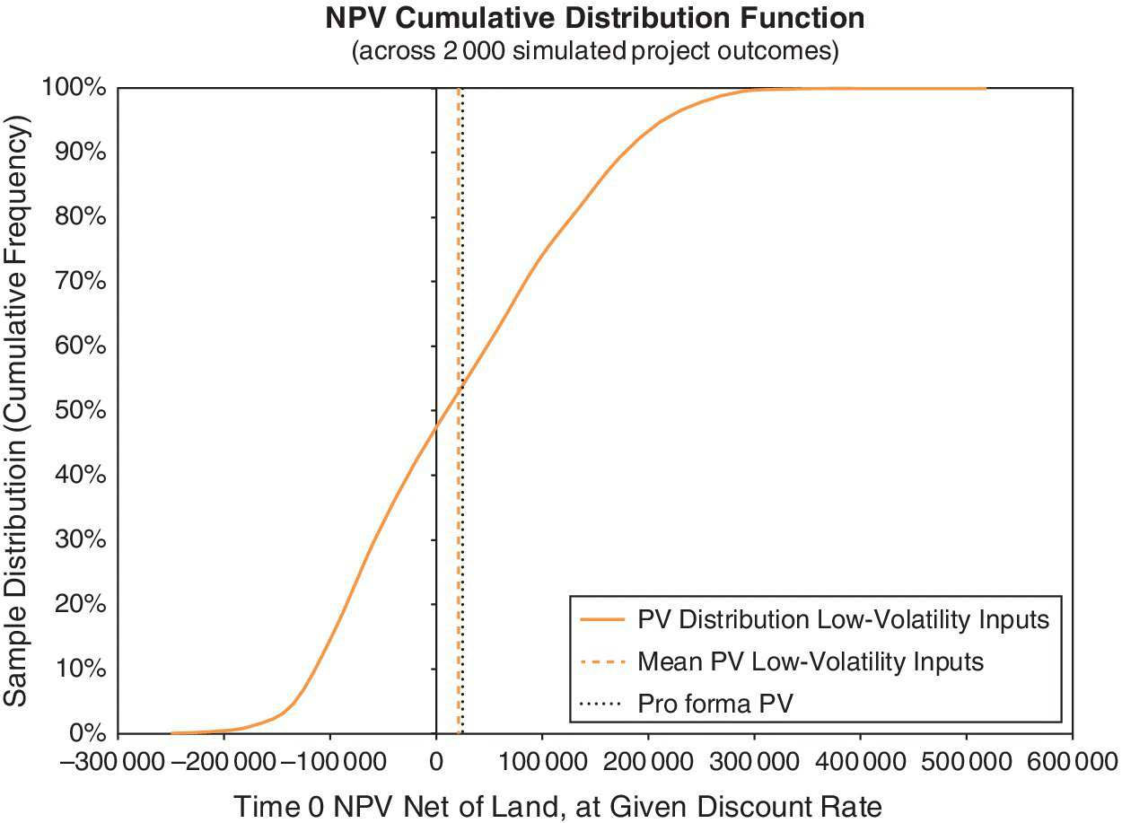
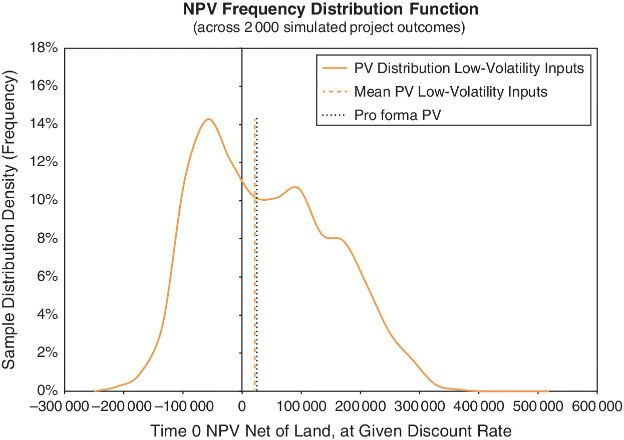
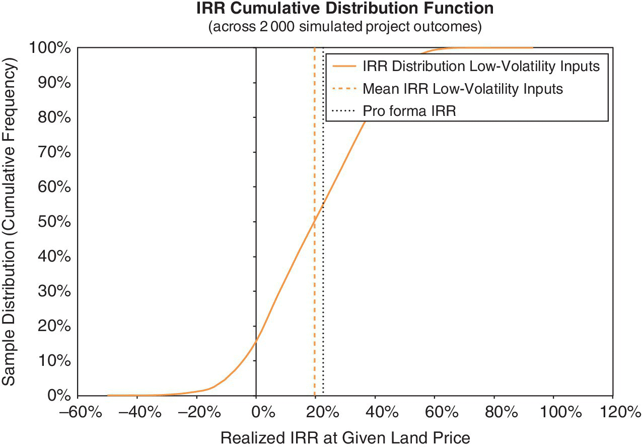
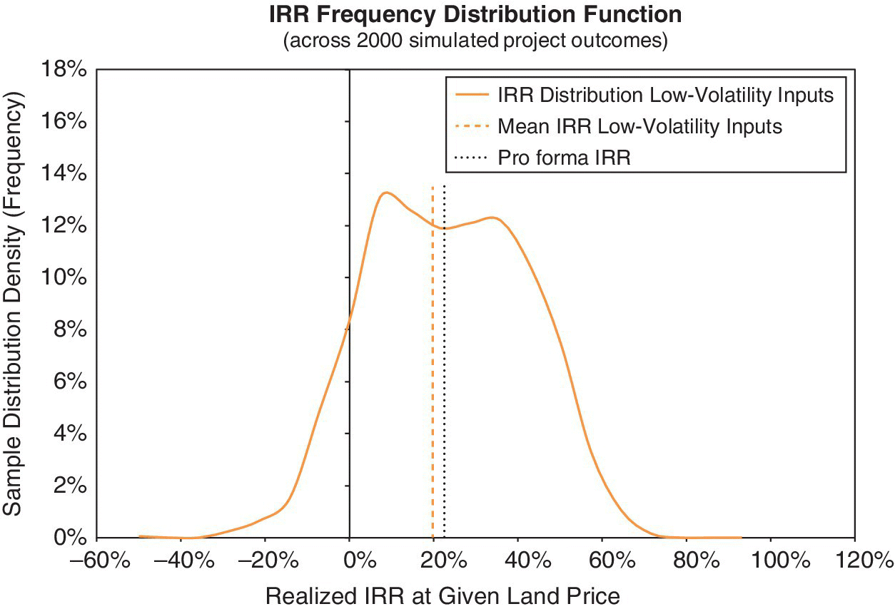
As noted in Chapter 7, any individual “run” of the simulation model (a single “recalculation” of the spreadsheet with many scenarios) produces a sample distribution of the possible future outcomes of the project. Such sample distributions of outputs are effectively estimates, as of Time 0, of the underlying ex‐ante probability distribution governing the project’s future investment performance. Normally, Time 0 is the time we plan to begin construction. Each time we run the simulation model, we generate a different sample, and no two runs will produce identical target curves. We strive for a sample size large enough that the target curves are quite stable for practical purposes, between simulation runs.
We depict the results graphically using either cumulative or frequency target curves (Chapter 8). The graphs in Figures 17.1–17.4 quantify and qualify the future uncertainty. They greatly enrich the picture provided by the classical single‐stream pro forma and by the traditional economic analysis of the project that was described in Section 16.5. That traditional approach is, at best, only a depiction of the average, or probabilistic, expectation of the future, based on estimates of the ex‐ante means of the cash flow probability distributions as reflected in the pro forma.
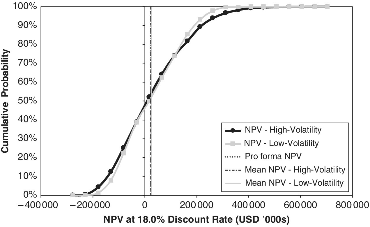
Regarding the NPV of the project (net of the given $200M land price), Figures 17.1 and 17.2 suggest that the future outcome probability has a slight positive skew around an expected value that is essentially the same as the single‐stream pro forma NPV. (The right‐hand tails are slightly longer than the left‐hand tails.) This is the same type of result as we noted in Chapter 8 regarding investments in existing assets. There, we were looking at the PV distribution, because we were valuing an existing built asset; and here, we are looking at the NPV distribution, because we are subtracting out land and construction costs to value a development project. Without any flexibility in the implementation of the project, the probability distribution has the same general characteristics for the money‐valued target metric. This is because present values are linear functions of future cash flows, which mathematically makes the mean of a distribution of future PVs equal to the PV of the mean of the future cash flows.
In Figures 17.1 and 17.2, the dashed, gray, vertical line is essentially at the same value as the dotted black line of the traditional pro forma NPV for the project, as reported in Chapter 16. The dashed, gray, vertical line is the sample mean of the simulation output distribution for the run depicted in the chart. As noted, there will always be some minor variation in sample statistics around true values. The sample mean NPV and the pro forma NPV are very close, and not statistically significantly different. In principle, we expect these two NPVs to be the same, owing to the linearity of the present value function, and because our random cash flow pricing factors are neutral and centered around the base case, since we are treating the base case pro forma as being unbiased.
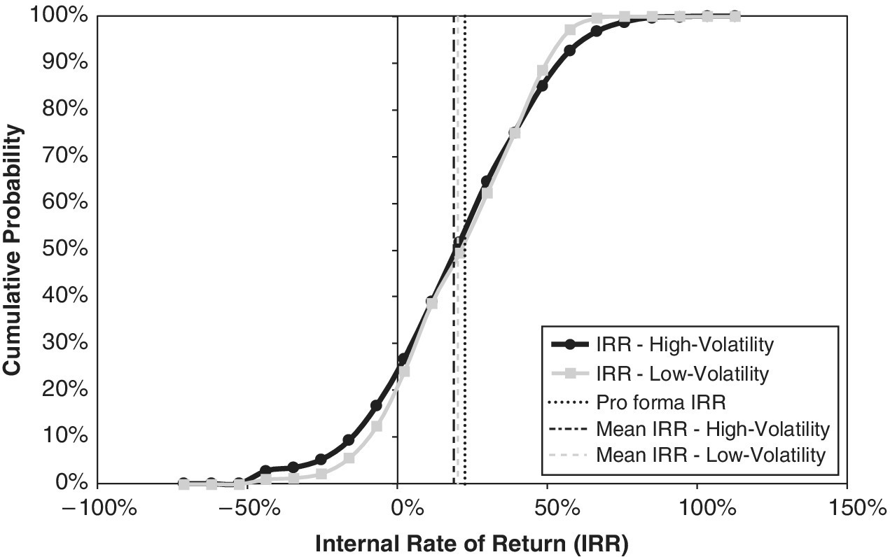
Also, similar to the Chapter 8 results, the ex‐post (realized) IRR distribution (based on the given land price) tends to be symmetric, as Figures 17.3 and 17.4 reveal. But, just as in Chapter 8, the mean ex‐post‐realized IRR in the Monte Carlo simulation is slightly below the 22.6% going‐in IRR that was indicated in the traditional pro forma of Chapter 16. The sample mean IRR is about 20%. Notice that the dashed, gray, vertical lines in Figures 17.3 and 17.4 (the sample mean IRR) are noticeably and statistically significantly to the left of the dotted black vertical lines (the pro forma IRR).
Furthermore, the simulation reveals that the standard deviation in the achieved IRR is approximately 23%. It suggests that there is an approximately 5% chance, 5% value at risk, that the actually realized IRR will be less than negative 16%. Investors are often interested in the tails of the future possibilities. As we repeatedly emphasize, in order to appreciate fully the implications of uncertainty, and especially in order to analyze and evaluate flexibility, we need to work with the entire future probability distribution. This is what the simulation model allows us to do.
The difference between the realistic IRR based on the distribution of uncertainty and the IRR based on a single average case is a typical result. It reflects the “flaw of averages” point made in Section 5.4: the average of a non‐linear function does not necessarily equal the value of that function evaluated at the average. (On average, houses don’t burn down, but the mortgage lender still requires you to buy fire insurance.) In the absence of flexibility, the IRR, as a function of the NPV, curves downwards (it is concave).
The scatterplot of the Garden City simulation results demonstrates this curvature (Figure 17.5). It shows the IRR as a function of the NPV of the project. Each point in the graph indicates the Garden City IRR and NPV results for one of the 2000 simulated future scenarios. The NPV result is on the horizontal axis, and the IRR result is on the vertical axis. The points, of course, spread out randomly, including a few outliers, but the central shape of the “cloud” is that of a curve that bends downwardly over the NPV values on the horizontal axis. This is why, and how, the expected IRR is less than the pro forma IRR of the expected cash flows. This biases the pro forma IRR, which is the IRR of the average cash flows, to be greater than the average of the probability distribution of the ex‐post IRRs, the more so the greater the uncertainty in the future cash flows.
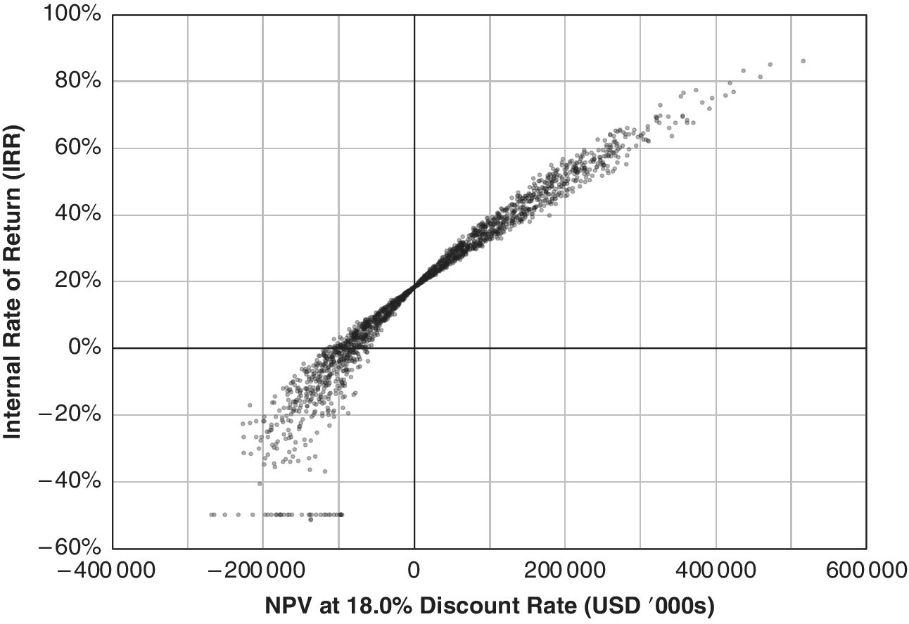
Figure 17.5 Garden City simulation results reflecting uncertainty without flexibility: IRR as a function of NPV.
17.4 Effect of Different Probability Inputs Assumptions
The results shown in Figures 17.1–17.4 derive from pricing factors that reflect input assumptions about real estate price dynamics. The authors believe that these are realistic and that they reflect typical real estate markets. We present and discuss our specific input assumptions in the Appendix. But real estate price dynamics differ over time and across different real estate markets. And no one ever knows the exact “true” price dynamics assumptions to input into the simulation model.
We should thus always be “humble” in using and presenting simulation analyses. We should always recognize that they will contain error, and we should never ignore common sense. We should consider how other assumptions might affect results.
To illustrate such a sensitivity analysis, we repeat the simulation of the Garden City project, assuming higher volatility in our real estate market pricing dynamics. Specifically, we ran the analysis using annual volatility in the real estate market of about 23%, measured for existing property assets without leverage. We label this as a “high‐volatility” assumption. We compare it to the previous results, which we obtained using a “low‐volatility” assumption of around 17%. Both these assumptions are within the plausible range for the volatility that individual property assets experience.
Figures 17.6–17.9 contrast the results of the high‐ and low‐volatility assumptions. The high‐volatility inputs assumption results in project performance output distributions that are slightly more spread out, reflecting greater investment risk (other things being equal). This is seen in the greater range or spread in the target curves (they are “flatter” over the range of output values on the horizontal axes). However, the effects of the alternative assumptions are not terribly large. There is no effect on the mean NPV, and only a slight effect on the mean IRR. (The thin, black, dashed line representing the mean outcome with the high‐volatility assumption is slightly to the left of the thicker, dashed, gray line representing the mean of the low‐volatility assumption.) In principle, greater volatility reduces the mean IRR, due to the previously noted concavity effect (and the “Jensen’s Inequality” rule, discussed in Section 5.4). Increasing the input volatility assumption increases the sample standard deviation of the realized IRR, which we could view as a measure of investment risk, from about 23% to about 27%. This spread is around the mean realized IRR of approximately 20% under the low‐volatility assumption and 19% under the high‐volatility assumption. (Recall that the pro forma IRR is 22.6%.)


17.5 Conclusion
This chapter showed how we can analyze future uncertainty by embedding the traditional DCF pro forma of our example Garden City development project into a Monte Carlo simulation spreadsheet model. We discussed the nature of the resulting simulation for the development project, including the typical target probability distributions, and the effects of varying input assumptions about the nature of the uncertainty.
The results we see with our Garden City example reflect the general principles about the relationship between uncertainty and basic investment performance metrics—such as the implication that expected IRRs are less than the pro forma IRR based on the project’s expected cash flows.
In the following chapters, we introduce flexibility into our simulation of the value the Garden City project under uncertainty, which we explored in this chapter.
