Chapter 9

Neural Networks

Validation Methods

Hidden Layer Structure

Fitting Options

Data Preparation

An Example

Summary

References

Exercises

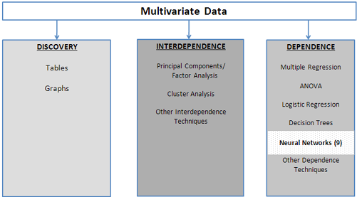
The Neural Networks technique as shown in our multivariate analysis framework in Figure 9.1 is one of the dependence techniques. Neural networks were originally developed to understand biological neural networks and were specifically studied by artificial intelligence researchers to allow computers to develop the ability to learn. In the past 25 years, neural networks have been successfully applied to a wide variety of problems, including predicting the solvency of mortgage applicants, detecting credit card fraud, validating signatures, forecasting stock prices, speech recognition programs, predicting bankruptcies, mammogram screening, determining the probability that a river will flood, and countless others.

Figure 9.1  A Framework for Multivariate Analysis

Neural networks are based on a model of how neurons in the brain communicate with each other. In a very simplified representation, a single neuron takes signals/inputs (electrical signals of varying strengths) from an input layer of other neurons, weights them appropriately, and combines them to produce signals/outputs (again, electrical signals of varying strengths) as an output layer, as shown in Figure 9.2. While this figure shows two outputs in the output layer, most applications of neural networks have only a single output.

Figure 9.2  A Neuron Accepting Weighted Inputs

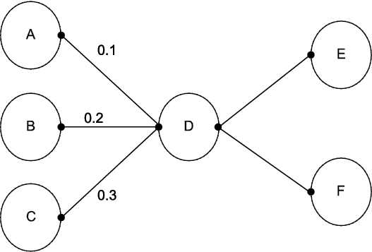
To make things easy, see Figure 9.3 below. Suppose that the strength of each signal emanating from neurons A, B, and C equals one. Now D might accept input from A with a weight of 0.1, from B with a weight of 0.2, and from C with a weight of 0.3. Then the output from D would be 0.1(1) + 0.2(1) + 0.3(1) = 0.6. Similarly, neurons E and F will accept the input of 0.6 with different weights. The linear activation function (by which D takes the inputs and combines them to produce an output) looks like a regression with no intercept. If we add what is called a “bias term” of 0.05 to the neuron D as shown in Figure 9.3, then the linear activation function by which D takes the inputs and produces an output is: output =0.05 + 0.1(1) +0.2(1) + 0.3(1) = 0.65.

Figure 9.3  A Neuron with a Bias Term

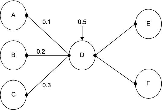
More generally, if Y is the output and the inputs are X1, X2, and X3, then the activation function could be written: Y = 0.05 + 0.1*X1 + 0.2*X2 +0.3*X3. Similarly, neurons E and F would have their own activation functions.

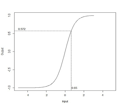
The activation functions used in neural networks are rarely linear as in the above examples, and are usually nonlinear transformations of the linear combination of the inputs. One such nonlinear transformation is the hyperbolic tangent, tanh, which would turn the value 0.65 into 0.572 as shown in Figure 9.4. Observe that in the central region of the input, near zero, the relationship between the input and the output is nearly linear; 0.65 is not that far from 0.572. However, farther away from zero, the relationship becomes decidedly nonlinear. Another common activation function is the Gaussian radial basis function.

Figure 9.4  Hyperbolic Tangent Activation Function

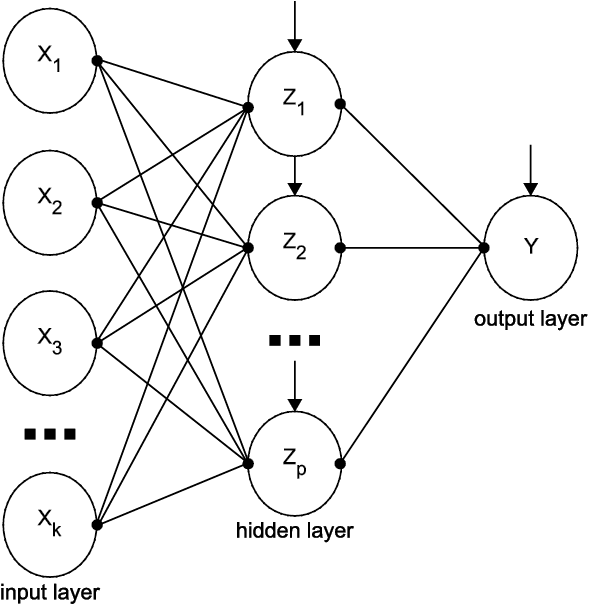
In practice, neural networks are slightly more complicated than those shown in Figures 9.2 and 9.3 and usually look like Figure 9.5 below. Rather than move directly from input to output, to obtain modeling flexibility, the inputs (what we call the X’s in a regression problem) are transformed into, say, features (i.e., nodes labeled as Z in the figure below; these are new variables that are combinations of the input variables). Then these variables are used as the inputs that produce the output.

To achieve this goal of flexibility, between the input and output layers is a hidden layer that models the features (i.e., creates new variables). As usual, let X represent inputs, Y represent outputs, and let Z represent features. A typical representation of such a neural network is given in Figure 9.5. Let there be k input variables, p features (which means p nodes in the hidden layer), and a single output. Each node of the input layer connects to each node of the hidden layer. Each of these connections has a weight, and each hidden node has a bias term. Each of the hidden nodes has its own activation function that must be chosen by the user.

Similarly, each node of the hidden layer connects to the node in the output layer, and the output node has a bias term. The activation function that produces the output is not chosen by the user: if the output is continuous, it will be a linear combination of the features and if the output is binary, it will be based on a logistic function as discussed in Chapter 5.

Figure 9.5 A Standard Neural Network Architecture

A neural network with k inputs, p hidden nodes, and 1 output has p(k+2)+1 weights to be estimated. So if k= 20 inputs and p=10 hidden nodes, then there are 221 weights to be estimated. How many observations are needed for each weight? It depends on the problem and is, in general, an open question with no definitive answer. But suppose it’s 100. Then you need 22,100 observations for such an architecture.

The weights for the connections between the nodes are initially set to random values close to zero and are modified (i.e., trained) on an iterative basis. By default, the criterion for choosing the weights is to minimize the sum of squared errors; this is also called the least squares criterion. The algorithm chooses random numbers close to zero as weights for the nodes, and creates an initial prediction for the output. This initial prediction is compared to the actual output, and the prediction error is calculated. Based on the error, the weights are adjusted, and a new prediction is made that has a smaller sum of squared errors than the previous prediction. The process stops when the sum of squared errors is sufficiently small.

The phrase “sufficiently small” merits elaboration. If left to its own devices, the neural network will make the error smaller and smaller on subsequent iterations, changing the weights on each iteration, until the error cannot be made any smaller. In so doing, the neural network will overfit the model (see Chapter 10 for an extended discussion of this concept) by fitting the model to the random error in the data. Essentially, an overfit model will not generalize well to other data sets. To combat this problem, JMP offers two validation methods: holdback and cross-validation.

Validation Methods

In traditional statistics, and especially in the social sciences and business statistics, one need only run a regression and report an R² (this is a bit of an over-simplification, but not much). Little or no thought is given to the idea of checking how well the model actually works. In data mining, it is of critical importance that the model “works;” it is almost unheard of to deploy a model without checking whether the model actually works. The primary method for doing this checking is called “validation.”

The holdback validation method works in the following way. The data set is randomly divided into two parts, the training sample and the validation (holdback) sample. Both parts have the same underlying model, but each has its own unique random noise. The weights are estimated on the training sample, and these weights are then used on the holdback sample to calculate the error. It is common to use 2/3 of the data for the training and 1/3 for the validation. Initially, as the algorithm iterates, the error on both parts will decline as the neural network learns the model that is common to both parts of the data set. After a sufficient number of iterations (i.e., recalculations of the weights) the neural network will have learned the model, and it will then begin to fit the random noise in the training sample. Since the holdback sample has different random noise, its calculated error will begin to increase.

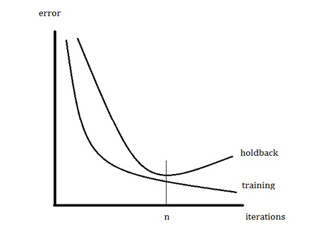
One way to view this relationship between the error (which we want to minimize) and the number of iterations is displayed in Figure 9.6. After n iterations, the neural network has determined the weights that minimize the error on the holdback sample. Any further iterations will only fit the noise in the training data and not the underlying model (and obviously will not fit the noise in the validation sample). Therefore, the weights based on n iterations that minimize the error on the holdout sample should be used. The curves in Figure 9.6 and the divergence between them as the number of iterations increases is a general method of investigating overfitting.

Figure 9.6  Typical Error Based on the Training Sample and the Holdback Sample

A second way to validate, called k-fold cross-validation, works in a different way to determine the number of iterations at which to stop, but the basic idea is the same. Divide the data set into k groups, or folds, that contain approximately the same number of observations. Consider k-1 folds to be the training data set, and the kth fold to be the validation data set. Compute the relevant measure of accuracy on the validation fold. Repeat this k times, each time leaving out a different fold, thus obtaining k measures of accuracy. Average the k measures of accuracy to obtain an overall estimate of the accuracy. As with holdback validation, to avoid overfitting, compare the training error to the validation error. Cross-validation is most often used when there are not enough data.

If randomly splitting the data set into two parts is not desirable for some reason, there is a third way to divide the data into training and validation samples. The user can manually split the data into two parts by instructing JMP to include specific rows for the training sample and excluding others that will constitute the holdback sample. There are two ways to do this.

First, the user can select some observations in the data table, right-click, and set them to Exclude. Then, when executing a neural net, under Validation Method, the user can choose Excluded Rows Holdback. Second, the user creates a new variable that indicates by zeros and ones whether a particular observation should be for training (zero) or validation (one). In the Neural dialog box when variables are cast as Y or X, the user will also set a variable as Validation. It will automatically be used for the validation method.

Hidden Layer Structure

Figure 9.5 shows a neural network architecture with one hidden layer that has p nodes. The nodes do not all have to have the same activation function. They can have any combination of the three types of activation functions, tanh, linear, or Gaussian. For example, six nodes in the hidden layer could have all tanh, or could have two each of the three types of the activation functions. Nor is the network limited to one hidden layer: JMP allows up to two hidden layers.

Concerning the architecture of a neural network, the two fundamental questions are: how many nodes for the input layer and how many nodes for the output layer? For the former, the number of variables is the answer. This number cannot be large for two reasons. First, a large number of variables greatly increases the possibility of local optima and correspondingly decreases the probability of finding the global optimum. Second, as the number of variables increases, the amount of time it takes to solve the problem increases even more. A tree or a logistic regression can easily accommodate hundreds of variables. A neural network might not be able to tolerate tens of variables, depending on the sample size and also depending on how long you can wait for JMP to return a solution. The number of nodes in the output layer depends on the problem. To predict a single continuous variable or a binary variable, use one output node. For a categorical variable with five levels, use five output nodes, one for each level.

Suppose there is only a single hidden layer. The guiding principle for determining the number of nodes is that there should be enough nodes to model the target variable, but not so many as to overfit. There are many rules of thumb to follow. Some of which are to set the number of nodes:

■ to be between the number of inputs and the number of outputs

■ to equal the number of inputs plus the number of outputs times 2/3

■ to be no more than twice the number of inputs

■ to be approximately ln(T) where T is the sample size

■ to be between 5% and 10% of the number of variables

The above list is a set of rules of thumb; notice that the first and second are contradictory. We do not give citations for these rules of thumb because they are all, in some sense, misleading. The fact is that there is no widely accepted procedure for determining the number of nodes in a hidden layer, and there is no formula that will give a single number to answer this question. (Of course, good advice is to find an article that describes successful modeling of the type in question, and use that article as a starting point.)

The necessary number of hidden nodes is a function of, among other things, the sample size, the complexity of the function to be modeled (and this function is usually unknown!), and the amount of noise in the system (which we cannot know unless we know the function!). With too few hidden nodes, the network cannot learn the underlying model and therefore cannot make good predictions on new data; but with too many nodes, the network memorizes the random noise (overfits) and cannot make good predictions on new data. Yoon et al. (1994) indicate that performance improves with each additional hidden node up to a point, after which performance deteriorates.

Therefore, a useful strategy is to begin with some minimum number of hidden nodes and increase the number of hidden nodes, keeping an eye on prediction error via the holdback sample or cross-validation, adding nodes as long as the prediction error continues to decline, and stopping when the prediction error begins to increase. If the training error is low and the validation error (either holdback or k-fold cross-validation) is high, then the model has been overfit, and the number of hidden nodes should be decreased. If both the training and validation errors are high, then more hidden nodes should be added. If the algorithm will not converge, then increase the number of hidden nodes. The bottom line is that extensive experimentation is necessary to determine the appropriate number of hidden nodes. It is possible to find successful neural network models built with as few as three nodes (predicting river flow) and as many as hundreds of hidden nodes (speech and handwriting recognition). The vast majority of analytics applications of neural networks seen by the authors have fewer than thirty hidden nodes.

The number of hidden layers is usually one. The reason to use a second layer is because it greatly reduces the number of hidden nodes that are necessary for successful modeling (Stathakis, 2009). There is little need to resort to using the second hidden layer until the number of nodes in the first hidden layer has become untenable—i.e., the computer fails to find a solution or takes too long to find a solution. However, using two hidden layers makes it easier to get trapped at a local optimum, which makes it harder to find the global optimum.

Boosting is an option that can be used to enhance the predictive ability of the neural network. Boosting is one of the great statistical discoveries of the 20^th century. A simplified discussion follows. Consider the case of a binary classification problem (e.g., zero or one). Suppose we have a classification algorithm that is a little better than flipping a coin; e.g., it is correct 55% of the time. This is called a weak classifier. Boosting can turn a weak classifier into a strong classifier.

The method of boosting is to run the algorithm once where all the observations have equal weight. In the next step, give more weight to the incorrectly classified observations and less weight to the correctly classified observations, and run the algorithm again. Repeat this re-weighting process until the algorithm has been run T times, where T is the “Number of Models” that the user specifies. Each observation then has been classified T times. If an observation has been classified more times as a zero than a one, then zero is its final classification; if it has been classified more times as a one, then that is its final classification. The final classification model, which uses all T of the weighted classification models, is usually more accurate than the initial classification, sometimes much more accurate. It is not unusual to see the error rate (the proportion of observations that are misclassified) drop from 20% on the initial run of the algorithm to below 5% for the final classification.

Boosting methods have also been developed for predicting continuous target variables. Gradient boosting is the specific form of boosting used for neural networks in JMP, and a further description can be found in the JMP help files. In the example in the manual, a 1-layer/2-node model is run when T=6, and the “final model” has 1 layer and 2x6=12 nodes (individual models are retained and combined at the end), which corresponds to the general method described above in the sense that the T re-weighted models are combined to form the final model.

The method of gradient boosting requires a learning rate, which is a number greater than zero and less than or equal to one. The learning rate describes how quickly the algorithm learns: the higher the learning rate, the faster the method converges, but a higher learning rate also increases the probability of overfitting. When the Number of Models (T) is high, then the learning rate should be low, and vice versa.

Fitting Options

One approach to improving the fit of the model is to transform all the continuous variables to near normality. This can be especially useful when the data contain outliers or are heavily skewed and is recommended in most cases. JMP offers two standard transformation methods, the Johnson Su and Johnson Sb methods. JMP automatically selects the preferred method.

In addition to the default least squares criterion, which minimizes the sum of squared errors, another criterion can be used to choose the weights for the model. The robust fit method minimizes the absolute value of the errors rather than the squared errors. This can be useful when outliers are present, since the estimated weights are much more sensitive to squared errors than absolute errors in the presence of outliers.

The penalty method combats the tendency of neural networks to overfit the data by imposing a penalty on the estimated weights, or coefficients. Some suggestions for choosing penalties follow. For example, the squared method penalizes the square of the coefficients. This is a good choice if you think that most of your inputs contribute to predicting the output; this is the default. The absolute method penalizes the absolute value of the coefficients, and this can be useful if you think that only some of your inputs contribute to predicting the output. The weight decay method can be useful if you think that only some of your inputs contribute to predicting the output. The no penalty option is much faster than the penalty methods, but it usually does not perform as well as the penalty methods because it tends to overfit.

As mentioned previously, to begin the iterative process of estimating the weights for the model, the initial weights are random numbers close to zero. Hence, the final set of weights is a function of the initial, random weights. It is this nature of neural networks to be prone to having multiple local optima that makes it easy for the minimization algorithm to find a local minimum for the sum of squared errors, rather than the global minimum. One set of initial weights can cause the algorithm to converge to one local optimum, while another set of initial weights might lead to another local optimum. Of course, we seek not local optima but the global optimum, and we hope that one set of initial weights might lead to the global optimum.

To guard against finding a local minimum instead of the global minimum, it is customary to restart the model several times using different sets of random initial weights, and then to choose the best of the several solutions. Using the Number of Tours option, JMP will do this automatically, so that the user does not need to do the actual comparison by hand. Each “tour” is a start with a new set of random weights. A good number to use is 20 (Sall, Creighton, and Lehman, 2007, p.468).

Data Preparation

Data with different scales can induce instability in neural networks (Weigend and Gershenfeld, 1994). Even if the network remains stable, having data with unequal scales can greatly increase the time necessary to find a solution. For example, if one variable is measured in thousands and another in units, the algorithm will spend more time adjusting for variation in the former rather than the latter. Two common scales for standardizing the data are:

(1) where s is the sample standard deviation, and

though other methods exist. Simply for ease, we prefer (1) since it is automated in JMP. (Select Analyze→Distribution and after the distribution is plotted, click the red triangle next to the variable name, and select Save→Standardized.) Another way is, when creating the neural network model, check the box for Transform Covariates under Fitting Options.

In addition to scaling, the data must be scrubbed of outliers. Outliers are especially dangerous for neural networks, because the network will model the outlier rather than the bulk of the data—much more so than, say, with logistic regression. Naturally, outliers should be removed before the data are scaled.

A categorical variable with more than two levels can be converted to dummy variables. But this means adding variables to the model at the expense of making the network harder to train and needing more data.

It is not always the case that categorical variables should be turned into dummy variables. First, especially in the context of neural networks that cannot handle a large number of variables, converting a categorical variable with k categories creates more variables. Doing this conversion with a few categorical variables can easily make the neural network model too difficult for the algorithm to solve. Secondly, conversion to dummy variables can destroy an implicit ordering of the categories that, when maintained, prevents the number of variables from being needlessly multiplied (as happens when converting to dummy variables). Pyle (1999, p. 74) gives an example where a marital status variable with five categories (married, widowed, divorced, single, or never married), instead of being converted to dummy variables, is better modeled as a continuous variable in the [0,1] range as shown in Table 9.1.

Table 9.1  Converting an Ordered Categorical Variable to [0,1]

Never Married

0

Single

0.1

Divorced

0.15

Widowed

0.65

Married

1.0

This approach is most useful when the levels of the categorical variable embody some implicit order. For example, if the underlying concept is “marriedness,” then someone who is divorced has been married more than someone who has never been married. A “single” person may be “never,” “divorced,” or “widowed,” but we don’t know which. Such a person is more likely to have experienced marriage than someone who has never been married. See Pyle (1999) for further discussion.

Neural networks are not like a tree or a logistic regression, both of which are useful in their own rights—the former as a description of a data set, the latter as a method of describing the effect of one variable on another. The only purpose of the neural network is for prediction. In the context of predictive analytics, we will generate predictions from a neural network and compare these predictions to those from trees and logistic regression, and then we will use the model that predicts the best. The bases for making these comparisons are the confusion matrix, ROC and lift curves, and various measures of forecast accuracy for continuous variables. All these are explained in the next chapter.

An Example

The Kuiper.JMP data set comes from Kuiper (2008), and contains the prices of 804 used cars and several variables thought to affect the price. The variable names are self-explanatory, and the interested reader can consult the article (available free and online) for further details. To keep the analysis simple, we will focus on one continuous target variable (Price), two continuous dependent variables (Mileage and Liter) and four binary variables (Doors, Cruise, Sound, and Leather). We ignore the other variables (e.g., Model and Trim). It will probably be easier to run the analyses if variables are defined as “y” or “x.”

In the data table, right-click on a variable, select Preselect Role, and then select Y for Price and X for Mileage, Liter, Doors, Cruise, Sound, and Leather.

As a baseline for our neural network modeling efforts, let us first run a linear regression. Of course, before running a regression, we must first examine the data graphically. A scatterplot (select Graph→Scatterplot Matrix) shows a clear group of observations near the top of most of the plots. Clicking them indicates that these are observations 151-160. Referring to the data set, we see that these are the Cadillac Hardtop Conv 2D cars. Since these cars appear to be outliers, let us exclude them from the analysis. Select these rows, and then right-click and select Exclude/Unexclude. Check the linearity of the relationship (select Analyze→Fit Y by X). Click the red arrow on the Bivariate Fit of Price by Mileage and select Fit Line. Do the same for Bivariate Fit of Price by Liter. Linearity seems reasonable, so run the full regression. Select Analyze→Fit Model and click Run. The RSquare is 0.439881; let’s call it 0.44.

With a baseline established, let’s turn to the neural network approach. Since we have preselected roles for the relevant variables, they will automatically be assigned as dependent and independent variables. We do not have to select variables each time we run a model. Select Analyze→Modeling→Neural and get the object shown in Figure 9.7.

Figure 9.7  Neural Network Model Launch

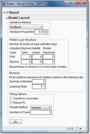
Notice the default options. The validation method is Holdback with a holdback proportion of 1/3. There is a single hidden layer with three nodes, each of which uses the tanh activation function. No boosting is performed, because the Number of Models is zero. Neither Transform Covariates nor Robust Fit is used, though the Penalty Method is applied with particular type of method being Squared. The model will be run only once, because Number of Tours equals one. Click Go.

Figure 9.8  Results of Neural Network Using Default Options

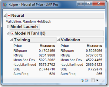
Your results will not be exactly like those in Figure 9.8 for two reasons. First, a random number generator is used to determine which 1/3 of the observations were used for the validation sample. Since your training and validation samples differ, so will your numerical results. Even if you had the same training and validation samples, your numerical results would still differ because your initial weights would be different. Remember that the neural network fitting of the weights is an iterative process that must begin somewhere, with some initial weights. These initial weights are random numbers near zero, produced by the JMP random number generator. Since your initial weights are different, your final weights will be different, too.

To get a feel for how much the results can vary, rerun the default neural network nine more times, keeping track of the training and validation RSquare each time. Click the red triangle for Model NTanH(3), and select Remove Fit. The Model Launch will reappear; then click Go. (You do not have to choose Remove Fit, but doing so cuts down on the number of results presented. Alternatively, you can click the triangle for Model Launch, and the Model Launch dialog box will reappear.) Our results are presented in Table 2, but remember that your results will differ.

Table 9.2  Training and Validation RSquare Running the Default Model Ten Times

Notice that the Training RSquare varies substantially, from a low of 46 to a high of 62. These many different solutions are a manifestation of the “multiple local optima” problem that is common to neural networks. Because the model is so highly nonlinear, there often will be several local optima when we really want the unique global optimum. To guard against mistakenly settling for a suboptimal result (e.g., the RSquare of 46 in Table 9.2), it is necessary to run the model several times. Since our goal is to get the best-fitting model on new data, we would naturally choose the model that has the RSquare of 62, as long as it was supported by the Validation RSquare. If the Validation RSquare was much lower than 58, we would take that to be evidence of overfitting and discard the model.

For this reason, JMP has the Number of Tours option that will automatically run the model several times and only report the model with the best RSquare. Typically, we expect to see a validation R² that is near the training R² if we have successfully modeled the data, or to see a validation R² that is much below the training R² if we have overfit the data. Occasionally, we can see a validation R² that is higher than the training R², as in the first column of Table 9.2 when the training R² is 46.

Now that we have some idea of what the default performance is, let’s try boosting the default model, setting the Number of Models option to 100. Results, shown in Table 9.3, are rather impressive. The average of the 10 training Rsquared values in Table 9.2 is 56.5. The average of the 10 training RSquare values in Table 9.3 is 67.4, an increase of more than 10 points. The downside is that boosting is designed to work with weak models, not strong models. While it can turn a mediocre model into a good model, as we see, it cannot turn a good model into a great model. Usually, one ought to be able to build a model good enough so that boosting won’t help. When, however, the best that can be done is a weak model, it’s nice to have the boosting method as a backup.

Table 9.3  Training and Validation RSquare When Boosting the Default Model, Number of Models = 100

Perhaps other options might improve the performance of the model on the validation data. Table 9.2 (and Table 9.3) shows run-to-run variation from changing initial coefficients for each run. After you click Go, the random draws that separate the data into training and validation for any particular run are fixed for the rest of the models that are run in the Neural report window. If this report window is closed and then the model is run again, the training and validation data will be different. To mitigate variation due to changing initial coefficients, we can select the Number of Tours option, which tries many different sets of initial coefficients and chooses the run with the best results. With respect to the difference between training and validation runs, we see that sometimes the R² is approximately the same, and other times one or the other is higher.

In what follows and, indeed, in what we have done so far, we must stress that no firm conclusions can be drawn concerning the superiority of one set of options when the number of runs equals only 5 or 10. There is no reason to rerun the model 100 times in the hope of obtaining definitive conclusions, because the conclusions would apply only to the data set being used. Hence, our conclusions are only tentative and conditional on the data being used.

Next let us compare transforming the variables as well as the method of validation. For this set of experiments, we will set the Number of Tours as 30. Results are presented in Table 9.4, where we use one hidden node with three tanh functions, and compare 10-fold cross-validation with 1/3 holdback sample on the car data, using the transform covariates option with Number of Tours =30.

Table 9.4 R2 for Five Runs of Neural Networks

We shall tentatively conclude that transforming produces better results than not transforming, as evidenced by the higher training R². (Take care to remember that five runs are far too few to draw such a conclusion.) Look at the untransformed results. If we only ran the model once and happened to get 74/66 (74 for training, 66 for validation) or 73/62, we might think that the architecture we chose overfit the data. Had we happened to get 75/76, we might think we had not overfit the data. This type of random variation in results must be guarded against, which means that the model must be run with many different architectures and many different options. And even then the same architecture with the same options should be run several times to guard against aberrant results.

In the best scenario when we finally have settled on a model and run it several times, all the training R² would be about the same, all the validation R² would be about the same, and the validation R² would be about the same as the training R² or perhaps a little lower. As for the present case in Table 9.4, we are far from the ideal situation. Between the training and validation data, sometimes the R² is approximately the same, sometimes it is higher for training, and sometimes it is higher for validation.

We have remarked on situations in which the validation R² is noticeably higher than the training R²; two such cases occur in Table 9.4. In particular, look at the transformed/k-fold case for 74/88, which has 714 observations in the training data and 80 in the validation data. This situation is usually the result of some observations with large residuals (one hesitates to call them “outliers”) that are in the training data not making it into the validation data. See the residuals plots for this case in Figures 9.9a (training data) and 9.9b (validation data). To make such plots, click the red triangle on Model and then select Plot Residual by Predicted.

Figure 9.9a  Residual Plot for Training Data When R2 = 74%

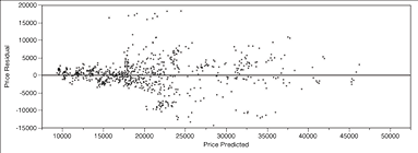
Figure 9.9b Residual Plot for Validation Data When R2 = 88%

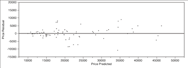
A big difference between these residual plots lies in the 15,000-25,000 range on the x-axis, and in the 15,000-20,000 range on the y-axis. The training data has residuals in this region that the validation data do not, and these are large residuals. Other such differences can be observed (e.g., between 20,000 and 35,000 on the x-axis, below the zero line). Hence, the big difference that we see in the R² between the two figures.

To be cautious, we should acknowledge that the Transform Covariates option might not satisfactorily handle outliers (we may have to remove them manually). Using a robust method of estimation might improve matters by making the estimates depend less on extreme values. For the validation methods, k-fold seems to have a higher R²; this might be due to a deficient sample size, or it might be due to a faulty model.

In Table 9.5 we vary the penalty. We set the Number of Tours option to 30, and select Transform Covariates, and set Holdback to 1/3, one hidden layer with three hidden nodes using the tanh activation function. Clearly, the Squared penalty produces the best results; so, moving forward, we will not use any other penalty for this data set.

Table 9.5 R2 for Different Penalty Functions 

Next we try changing the architecture as shown in Table 9.6. We use the Squared penalty, keep Number of Tours at 30, and select the Transform Covariates option. We increase the number of hidden nodes from three to four, five, and then ten, and finally change the number of hidden layers to two, each with six hidden nodes. All of these use the tanh function. Using 4 nodes represents an improvement over 3 nodes; and using 5 nodes represents an improvement over 4 nodes. Changing the architecture further produces only marginal improvements.

Table 9.6 R2 for Various Architectures 

Compared to linear regression (which had an R² of 0.44, you may recall), a neural network with one layer and five or ten nodes is quite impressive, as is the network with two layers and six nodes each.

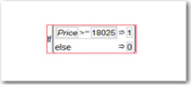
For the sake of completeness, let us briefly consider using the neural network to predict a binary dependent variable. Create a binary variable that equals one if the price is above the median and equals zero otherwise. That the median equals 18205 can be found by selecting Analyze→Distributions. To create the binary variable, select Cols→New Column, type MedPrice for the column name, click Column Properties, and select Formula. Under Functions, click Conditional and select If. The relevant part of the dialog box should look like Figure 9.9.

Figure 9.9  Creating a Binary Variable for Median Price

Click OK. In the data table, click on the blue y next to Price and change its role to No Role. Right-click MedPrice, choose Preselect Role, and select Y. Click the blue triangle next to MedPrice and change its type to Nominal. Select Analyze→Modeling→Neural and click Go. To see the confusion matrices (which were discussed briefly in Chapter Five and will be discussed in detail in the next chapter), click the triangles to obtain something like Figure 9.10. (Your results will be numerically different due to the use of the random number generator.)

Figure 9.10  Default Model for the Binary Dependent Variable, MedPrice

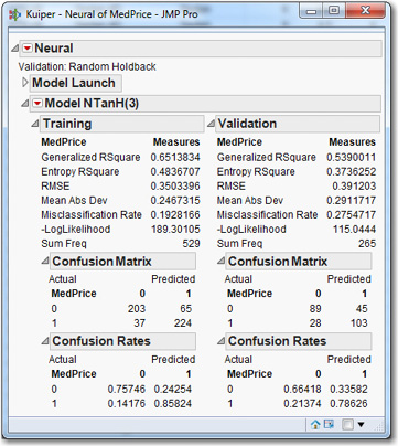
The correct predictions from the model, as shown in the Confusion Matrix, are in the upper left and lower right (e.g., 203 and 224). Looking at the Confusion Rates, we see that the correctly predicted proportions for zeros and ones are 0.75746 and 0.85824, respectively. These rates decline slightly in the validation sample (to 0.66418 and 0.78626), as is typical, because the model tends to overfit the training data.

Summary 

Neural networks are a black box, as far as statistical methods are concerned. The data go in, the prediction comes out, and nobody really knows what goes on inside the network. No hypotheses are tested, there are no p-values to determine whether variables are significant, and there is no way to determine precisely how the model makes its predictions. As such, neural networks, while they may be quite useful to a statistician, are probably not useful when one needs to present a model with results to a management team. The management team is not likely to put much faith in the statistician’s presentation: “We don’t know what it does or how it does it, but here is what it did.” At least trees are intuitive and easily explained, and logistic regression can be couched in terms of relevant variables and hypothesis tests, so these methods are better when one needs to present results to a management team.

Neural networks do have their strong points. They are capable of modeling extremely nonlinear phenomena, require no distributional assumptions, and they can be used for either classification (binary dependent variable) or prediction (continuous dependent variable). Selecting variables for inclusion in a neural network is always difficult, since there is no test for whether a variable makes a contribution to a model. Naturally, consultation with a subject-matter expert can be useful. Another way is to apply a tree to the data, and check the “variable importance” measures from the tree, and use the most important variables from the tree as the variables to be included in the neural network.

References

Kuiper, Shonda. (2008). “Introduction to Multiple Regression: How Much Is Your Car Worth?” Journal of Statistics Education, Vol. 16, No. 3.

Pyle, Dorian. (1999). Data Preparation for Data Mining. San Francisco: Morgan Kaufmann.

Sall, John, Lee Creighton, and Ann Lehman. (2007). JMP Start Statistics: A Guide to Statistics and Data Analysis Using JMP. 4^th Ed. Cary, NC: SAS Institute Inc.

Stathakis, D. (2009). “How many hidden layers and nodes?” International Journal of Remote Sensing. Vol. 30, No. 8, 2133–2147.

Weigend, A. S., and N. A. Gershenfeld (Eds.). (1994). Time Series Prediction: Forecasting the Future and Understanding the Past. Reading, MA: Addison-Wesley.

Yoon, Youngohc, Tor Guimaraes, and George Swales. (1994). “Integrating artificial neural networks with rule-based expert systems.” Decision Support Systems, 11(5), 497–507.

Exercises

1. Investigate whether the Robust option makes a difference. For the Kuiper data that has been used in this chapter (don’t forget to drop some observations that are outliers!), run a basic model 20 times (e.g., the type in Table 9.4). Run it 20 more times with the Robust option invoked. Characterize the difference between the results, if any. E.g., is there less variability in the R²? Is the difference between training R² and validation R² smaller? Now include the outliers, and redo the analysis. Has the effect of the Robust option changed?

2. For all the analyses of the Kuiper data in this chapter, ten observations were excluded because they were outliers. Include these observations and rerun the analysis that produced one of the tables in this chapter (e.g., Table 9.4). What is the effect of including these outliers?

3. For the neural net prediction of the binary variable MedPrice, try to find a suitable model by varying the architecture and changing the options.

4. Develop a neural network model for the Churn data.

5. In Chapter 8 we developed trees in two cases: a classification tree to predict whether students return, and a regression tree to predict GPA. Develop a neural network model for each case.

6. As indicated in the text, sometimes rescaling variables can improve the performance of a neural network model. Rescale the variables for an analysis presented in the chapter, or in the exercises, and see whether the results improve.