
Racial inequality in the 21st century: the declining significance of discrimination
Fryer Roland G. Jr.1, Harvard University, EdLabs, NBER
Abstract
There are large and important differences between blacks in whites in nearly every facet of life— earnings, unemployment, incarceration, health, and so on. This chapter contains three themes. First, relative to the 20th century, the significance of discrimination as an explanation for racial inequality across economic and social indicators has declined. Racial differences in social and economic outcomes are greatly reduced when one accounts for educational achievement; therefore, the new challenge is to understand the obstacles undermining the development of skill in black and Hispanic children in primary and secondary school. Second, analyzing ten large datasets that include children ranging in age from eight months old seventeen years old, we demonstrate that the racial achievement gap is remarkably robust across time, samples, and particular assessments used. The gap does not exist in the first year of life, but black students fall behind quickly thereafter and observables cannot explain differences between racial groups after kindergarten. Third, we providea brief history of efforts to close the achievement gap.
There are several programs—various early childhood interventions, more flexibility and stricter accountability for schools, data-driven instruction, smaller class sizes, certain student incentives, and bonuses for effective teachers to teach in high-need schools, which have a positive return on investment, but they cannot close the achievement gap in isolation. More promising are results from a handful of high-performing charter schools, which combine many of the investments above in a comprehensive framework and provide an “existence proof’’—demonstrating that a few simple investments can dramatically increase the achievement of even the poorest minority students. The challenge for the future is to take these examples to scale.
Keywords
Racial achievement gap; Charter schools; Racial inequality
“In the 21st Century, the best anti-poverty program around is a world-class education.”
President Barack Obama, State of the Union Address (January 27,2010)
1 Introduction
Racial inequality is an American tradition. Relative to whites, blacks earn twenty-four percent less, live five fewer years, and are six times more likely to be incarcerated on a given day. Hispanics earn twenty-five percent less than whites and are three times more likely to be incarcerated.2 At the end of the 1990s, there were one-third more black men under the jurisdiction of the corrections system than there were enrolled in colleges or universities (Ziedenberg and Schiraldi, 2002). While the majority of barometers of economic and social progress have increased substantially since the passing of the civil rights act, large disparities between racial groups have been and continue to be an everyday part of American life.
Understanding the causes of current racial inequality is a subject of intense debate. A wide variety of explanations—which range from genetics (Jensen, 1973; Rushton, 1995) to personal and institutional discrimination (Darity and Mason, 1998; Pager, 2007; Krieger and Sidney, 1996) to the cultural backwardness of minority groups (Reuter, 1945; Shukla, 1971)—have been put forth. Renowned sociologist William Julius Wilson argues that a potent interaction between poverty and racial discrimination can explain current disparities (Wilson, 2010).
Decomposing the share of inequality attributable to these explanations is exceedingly difficult, as experiments (field, quasi-, or natural) or other means of credible identification are rarely available.3 Even in cases where experiments are used (i.e., audit studies), it is unclear precisely what is being measured (Heckman, 1998). The lack of success in convincingly identifying root causes of racial inequality has often reduced the debate to a competition of “name that residual”—arbitrarily assigning identity to unexplained differences between racial groups in economic outcomes after accounting for a set of confounding factors. The residuals are often interpreted as “discrimination,” “culture,” “genetics,” and so on. Gaining a better understanding of the root causes of racial inequality is of tremendous importance for social policy, and the purpose of this chapter.
This chapter contains three themes. First, relative to the 20th century, the significance of discrimination as an explanation for racial inequality across economic and social indicators has declined. Racial differences in social and economic outcomes are greatly reduced when one accounts for educational achievement; therefore, the new challenge is to understand the obstacles undermining the achievement of black and Hispanic children in primary and secondary school. Second, analyzing ten large datasets that include children ranging in age from eight months old to seventeen years old, we demonstrate that the racial achievement gap is remarkably robust across time, samples, and particular assessments used. The gap does not exist in the first year of life, but black students fall behind quickly thereafter and observables cannot explain differences between racial groups after kindergarten.
Third, we provide a brief history of efforts to close the achievement gap. There are several programs—various early childhood interventions, more flexibility and stricter accountability for schools, data-driven instruction, smaller class sizes, certain student incentives, and bonuses for effective teachers to teach in high-need schools, which have a positive return on investment, but they cannot close the achievement gap in isolation.4 More promising are results from a handful of high-performing charter schools, which combine many of the investments above in a comprehensive model and provide a powerful “existence proof”—demonstrating that a few simple investments can dramatically increase the achievement of even the poorest minority students.
An important set of questions is: (1) whether one can boil the success of these charter schools down to a form that can be taken to scale in traditional public schools; (2) whether we can create a competitive market in which only high-quality schools can thrive; and (3) whether alternative reforms can be developed to eliminate achievement gaps. Closing the racial achievement gap has the potential to substantially reduce or eliminate many of the social ills that have plagued minority communities for centuries.
2 The declining significance of discrimination
One of the most important developments in the study of racial inequality has been the quantification of the importance of pre-market skills in explaining differences in labor market outcomes between blacks and whites (Neal and Johnson, 1996; O’Neill, 1990). Using the National Longitudinal Survey of Youth 1979 (NLSY79), a nationally representative sample of 12,686 individuals aged 14 to 22 in 1979, Neal and Johnson (1996) find that educational achievement among 15- to 18-year-olds explains all of the black-white gap in wages among young women and 70% of the gap among men. Accounting for pre-market skills also eliminates the Hispanic-white gap. Important critiques such as racial bias in the achievement measure (Darity and Mason, 1998; Jencks, 1998), labor market dropouts, or the potential that forward-looking minorities underinvest in human capital because they anticipate discrimination in the market cannot explain the stark results.5
We begin by replicating the seminal work of Neal and Johnson (1996) and extending their work in four directions. First, the most recent cohort of NLSY79 is between 42 and 44 years old (15 years older than in the original analysis), which provides a better representation of the lifetime gap. Second, we perform a similar analysis with the National Longitudinal Survey of Youth 1997 cohort (NLSY97). Third, we extend the set of outcomes to include unemployment, incarceration, and measures of physical health. Fourth, we investigate the importance of pre-market skills among graduates of thirty-four elite colleges and universities in the College and Beyond database, 1976 cohort.
To understand the importance of academic achievement in explaining life outcomes, we follow the lead of Neal and Johnson (1996) and estimate least squares models of the form:
![]() (1)
(1)
where i indexes individuals, Xi denotes a set of control variables, and Ri is a full set of racial identifiers.
Table 1 presents racial disparities in wage and unemployment for men and women, separately.6 The odd-numbered columns present racial differences on our set of outcomes controlling only for age. The even-numbered columns add controls for the Armed Forces Qualifying Test (AFQT)—a measure of educational achievement that has been shown to be racially unbiased (Wigdor and Green, 1991)—and its square. Black men earn 39.4% less than white men; black women earn 13.1% less than white women. Accounting for educational achievement drastically reduces these inequalities—39.4% to 10.9% for black men and 13.1% lower than whites to 12.7% higher for black women.7 An eleven percent difference between white and black men with similar educational achievement is a large and important number, but a small fraction of the original gap. Hispanic men earn 14.8% less than whites in the raw data—62% less than the raw black-white gap—which reduces to 3.9% more than whites when we account for AFQT. The latter is not statistically significant. Hispanic women earn six percent less than white women (not significant) without accounting for achievement. Adding controls for AFQT, Hispanic women earn sixteen percent more than comparable white women and these differences are statistically significant.
Table 1
The importance of educational achievement on racial differences in labor market outcomes (NLSY79).
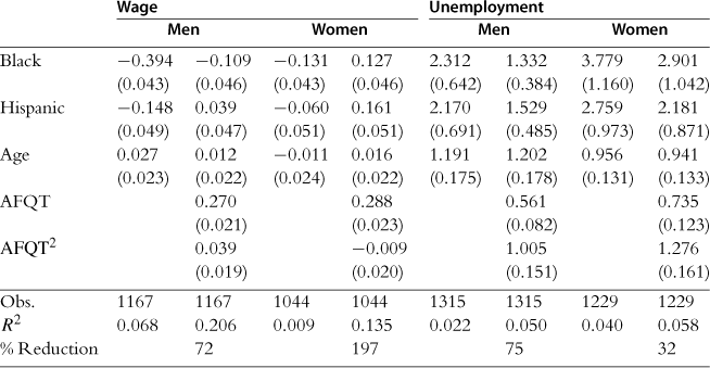
The dependent variable in columns 1 through 4 is the log of hourly wages of workers. The wage observations come from 2006. All wages are measured in 2006 dollars. The wage measure is created by multiplying the hourly wage at each job by the number of hours worked at each job that the person reported as a current job and then dividing that number by the total number of hours worked during a week at all current jobs. Wage observations below $1 per hour or above $115 per hour are eliminated from the data. The dependent variable in columns 5 through 8 is a binary variable indicating whether the individual is unemployed. The unemployment variable is taken from the individual’s reported employment status in the raw data. In both sets of regressions, the sample consists of the NLSY79 cross-section sample plus the supplemental samples of blacks and Hispanics. Respondents who did not take the ASVAB test are included in the sample and a dummy variable is included in the regressions that include AFQT variables to indicate if a person did not have a valid AFQT score. This includes 134 respondents who had a problem with their test according to the records. All included individuals were born after 1961. The percent reduction reported in even-numbered columns represents the reduction in the coefficient on black when controls for AFQT are added. Standard errors are in parentheses.
Labor force participation follows a similar pattern. Black men are more than twice as likely to be unemployed in the raw data and thirty percent more likely after controlling for AFQT. For women, these differences are 3.8 and 2.9 times more likely, respectively. Hispanic-white differences in unemployment with and without controlling for AFQT are strikingly similar to black-white gaps.
Table 2 replicates Table 1 using the NLSY97.8 The NLSY97 includes 8984 youths between the ages of 12 and 16 at the beginning of 1997; these individuals are 21 to 27 years old in 2006–2007, the most recent years for which wage measures are available. In this sample, black men earn 17.9% less than white men and black women earn 15.3% less than white women. When we account for educational achievement, racial differences in wages measured in the NLSY97 are strikingly similar to those measured in NLSY79— 10.9% for black men and 4.4% for black women. The raw gaps, however, are much smaller in the NLSY97, which could be due either to the younger age of the workers and a steeper trajectory for white males (Farber and Gibbons, 1996) or to real gains made by blacks in recent years. After adjusting for age, Hispanic men earn 6.5% less than white men and Hispanic women earn 5.7% less than white women, but accounting for AFQT eliminates the Hispanic-white gap for both men and women.
Table 2
The importance of educational achievement on racial differences in labor market outcomes (NLSY97).
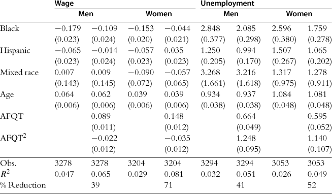
The dependent variable in columns 1 through 4 is the log of hourly wages of workers. The wage observations come from 2006 and 2007. All wages are measured in 2006 dollars. The wage measure for each year is created by multiplying the hourly wage at each job by the number of hours worked at each job that the person reported as a current job and then dividing that number by the total number hours worked during a week at all current jobs. If a person worked in both years, the wage is the average of the two wage observations. Otherwise the reported wage is from the year for which the individual has valid wage data. Wage observations below $1 per hour or above $115 per hour are eliminated from the data. The dependent variable in columns 5 through 8 is a binary variable indicating whether the individual is unemployed. The unemployment variable is taken from the individual’s reported employment status in the raw data. The employment status from 2006 is used for determining unemployment. The coefficients in columns 5 through 8 are odds ratios from logistic regressions. Respondents who did not take the ASVAB test are included in the sample and a dummy variable is included to indicate if a person did not have a valid AFQT score in the regressions that include AFQT variables. The percent reduction reported in even-numbered columns represents the reduction in the coefficient on black when controls for AFQT are added. Standard errors are in parentheses.
Black men in the NLSY97 are almost three times as likely to be unemployed, which reduces to twice as likely when we account for educational achievement. Black women are roughly two and a halftimes more likely to be unemployed than white women, but controlling for AFQT reduces this gap to seventy-five percent more likely. Hispanic men are twenty-five percent more likely to be unemployed in the raw data, but when we control for AFQT, this difference is eliminated. Hispanic women are fifty percent more likely than white women to be unemployed and this too is eliminated by controlling for AFQT. Similar to the NLSY79, controlling for AFQT has less of an impact on racial differences in unemployment than on wages.
Table 3 employs a Neal and Johnson specification on two social outcomes: incarceration and physical health. The NLSY79 asks the “type of residence” in which the respondent is living during each administration of the survey, which allows us to construct a measure of whether the individual was ever incarcerated when the survey was administered across all years of the sample.9 The NLSY97 asks individuals if they have been sentenced to jail, an adult corrections institution, or a juvenile corrections institution in the past year for each yearly follow-up survey of participants. In 2006, the NLSY79 included a 12-Item Short Form Health Survey (SF-12) for all individuals over age 40. The SF-12 consists of twelve self-reported health questions ranging from whether the respondent’s health limits him from climbing several flights of stairs to how often the respondent has felt calm and peaceful in the past four weeks. The responses to these questions are combined to create physical and mental component summary scores.
Table 3
The importance of educational achievement on racial differences in incarceration and health outcomes.

The dependent variable in columns 1 through 8 is a measure of whether the individual was ever incarcerated. In the NLSY79 data, this variable is equal to one if the individual reported their residence as jail during any of the yearly follow-up surveys or if they reported having been sentenced to a corrective institution before the baseline survey and is equal to zero otherwise. In the NLSY97 data, this variable is equal to one if the person reports having been sentenced to jail, an adult corrections institution, or a juvenile corrections institution in the past year during any of the yearly administrations of the survey and is equal to zero otherwise. The coefficients in columns 1 through 8 are odds ratios from logistic regressions. The dependent variable in columns 9 through 12 is the physical component score (PCS) reported in the NLSY79 derived from the 12-Item Short Form Health Survey of individuals over age 40. The PCS is standardized to have a mean of zero and a standard deviation of one. Individuals who do not have valid PCS data are not included in these regressions. In the NLSY79 regressions, included individuals were born after 1961. Respondents who did not take the ASVAB test are included in the sample and a dummy variable is included in the regressions that include AFQT variables to indicate if a person did not have a valid AFQT score. For NLSY79, this includes 134 respondent that had a problem with their test according to the records. The percent reduction reported in even-numbered columns represents the reduction in the coefficient on black when controls for AFQT are added. Standard errors are in parentheses.
Adjusting for age, black males are about three and a half times and Hispanics are about two and a half times more likely to have ever been incarcerated when surveyed.10 Controlling for AFQT, this is reduced to about eighty percent more likely for blacks and fifty percent more likely for Hispanics. Again, the racial differences in incarceration after controlling for achievement is a large and important number that deserves considerable attention in current discussions of racial inequality in the United States. Yet, the importance of educational achievement in the teenage years in explaining racial differences is no less striking.
The final two columns of Table 3 display estimates from similar regression equations for the SF-12 physical health measure, which has been standardized to have a mean of zero and standard deviation of one for ease of interpretation. Without accounting for achievement, there is a black-white disparity of 0.15 standard deviations in self-reported physical health for men and 0.23 standard deviations for women. For Hispanics, the differences are −0.140 for men and 0.030 for women. Accounting for educational achievement eliminates the gap for men and cuts the gap in half for black women [−0.111 (0.076)]. The remaining difference for black women is not statistically significant. Hispanic women report better health than white women with or without accounting for AFQT.
Extending Neal and Johnson (1996) further, we turn our attention to the College and Beyond (C&B) Database, which contains data on 93,660 full-time students who entered thirty-four elite colleges and universities in the fall of 1951, 1976, or 1989. We focus on the cohort from 1976.11 The C&B data contain information drawn from students’ applications and transcripts, Scholastic Aptitude Test (SAT) and the American College Test (ACT) scores, standardized college admissions exams that are designed to assess a student’s readiness for college, as well as information on family demographics and socioeconomic status in their teenage years.12 The C&B database also includes responses to a survey administered in 1995 or 1996 to all three cohorts that provides detailed information on post-college labor market outcomes. Wage data were collected when the respondents were approximately 38 years old, and reported as a series of ranges. We assigned individuals the midpoint value of their reported income range as their annual income.13 The response rate to the 1996 survey was approximately 80%. Table A.3 contains summary statistics used in our analysis.
Table 4 presents racial disparities in income for men and women from the 1976 cohort of the C&B Database.14 The odd-numbered columns present raw racial differences. The even-numbered columns add controls for performance on the SAT and its square.15 Black men from this sample earn 27.3% less than white men, but when we account for educational achievement, the gap shrinks to 15.2%. Black women earn more than white women by 18.6%, which increases to an advantage of 28.6% when accounting for SAT scores. There are no differences in income between Hispanics and whites with or without accounting for achievement.
Table 4
The importance of educational achievement on racial differences in labor market outcomes (C&B 76).
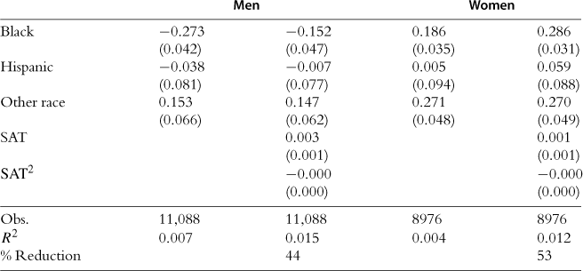
The dependent variable is the log of annual income. Annual income is reported as a series of ranges; each individual is assigned the midpoint of their reported income range as their annual income. Income data were collected for either 1994 or 1995. Individuals who report earning less than $1000 annually or who were students at the time of data collection are excluded from these regressions. Those individuals with missing SAT scores are included in the sample and a dummy variable is included in the regressions that include SAT variables to indicate that a person did not have a valid AFQT score. All regressions use institution weights and standard errors are clustered at the institution level. Standard errors are in parentheses.
In developing countries, eradicating poverty takes a large and diverse set of strategies: battling disease, fighting corruption, building schools, providing clean water, and so on (Schultz and Strauss, 2008). In the United States, important progress toward racial equality can be made if one ensures that black and white children obtain the same skills. This is an enormous improvement over the battles for basic access and equality that were fought in the 20th century, but we must now work to close the racial achievement gaps in education—high-quality education is the new civil rights battleground.16
3 Basic facts about racial differences in achievement before kids enter school
We begin our exploration of the racial achievement gap with data on mental function in the first year of life. This approach has two virtues. First, nine months is one of the earliest ages at which one can reliably test cognitive achievement in infants. Second, data on the first year of life provide us with a rare opportunity to potentially understand whether genetics is an important factor in explaining racial differences later in life.17
There are only two datasets that both are nationally representative and contain assessments of mental function before the first year of life. The first is the US Collaborative Perinatal Project (CPP) (Bayley, 1965), which includes over 31,000 women who gave birth in twelve medical centers between 1959 and 1965. The second dataset is the Early Childhood Longitudinal Study, Birth Cohort (ECLS-B), a nationally representative sample with measures of mental functioning (a shortened version of the Bayley Scale of Infant Development) for over 10,000 children aged one and under. Summary statistics for the variables we use in our core specifications are displayed by race in Table A.4 (CPP) and Table A.5 (ECLS-B).
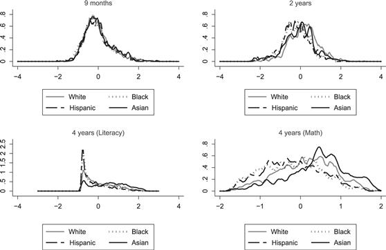
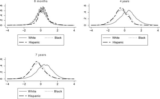
Figures 1 and 2 plot the density of mental test scores by race at various ages in the ECLS-B and CPP data sets, respectively.18 In Fig. 1, the test score distributions on the Bayley Scale at age nine months for children of different races are visually indistinguishable. By age two, the white distribution has demonstrably shifted to the right. At age four, the cognitive score is separated into two components: literacy (which measures early language and literacy skills) and math (which measures early mathematics skills and math readiness). Gaps in literacy are similar to disparities at age two; early math skills differences are more pronounced. Figure 2 shows a similar pattern using the CPP data. At age eight months, all races look similar. By age four, whites are far ahead of blacks and Hispanics and these differences continue to grow over time. Figures 1 and 2 make one of the key points of this section: the commonly observed racial achievement gap only emerges after the first year of life.
To get a better sense of the magnitude (and standard errors) of the change from nine months to seven years old, we estimate least squares models of the following form:
![]() (2)
(2)
where i indexes individuals, a indexes age in years, and Ri corresponds to the racial group to which an individual belongs. The vector Xi captures a wide range of possible control variables including demographics, home and prenatal environment; ε; a is an error term. The variables in the ECLS-B and CPP datasets are similar, but with some important differences.19 In the ECLS-B dataset, demographic variables include the gender of the child, the age of the child at the time of assessment (in months), and the region of the country in which the child lives. Home environment variables include a single socioeconomic status measure (by quintile), the mother’s age, the number of siblings, and the family structure (child lives with: “two biological parents,” “one biological parent,” and so on). There is also a “parent as teacher” variable included in the home environment variables. The “parent as teacher” score is coded based on interviewer observations of parent-child interactions in a structured problem-solving environment and is based on the Nursing Child Assessment Teaching Scale (NCATS). Our set of prenatal environment controls include: the birthweight of the child (in 1000-gram ranges), the amount premature that the child was born (in 7-day ranges), and a set of dummy variables representing whether the child was a single birth, a twin, or one in a birth of three or more.
In the CPP dataset, demographic variables include the age of the child at the time of assessment (in months) and the gender of the child. Our set of home environment variables provides rich proxies of the environment in which children were reared. The set of home variables includes: parental education (both mother’s and father’s, which have been transformed to dichotomous variables ranging from “high school dropout” to “college degree or more”), parental occupation (a set of mutually exclusive and collectively exhaustive dummy variables: “no occupation,” “professional occupation,” or “non-professional occupation”), household income during the first three months of pregnancy (in $500 ranges), mother’s age, number of siblings, and each mother’s reaction to and interactions with the child, which are assessed by the interviewer (we indicate whether a mother is indifferent, accepting, attentive, over-caring, or if she behaves in another manner). The set of prenatal environment controls for the CPP is the same as the set of prenatal environment controls in the ECLS-B dataset. Also included in the analysis of both datasets is interviewer fixed effects, which adjust for any mean differences in scoring of the test across interviewers.20 It is important to stress that a causal interpretation of the coefficients on the covariates is likely to be inappropriate; we view these particular variables as proxies for a broader set of environmental and behavioral factors.
The coefficients on the race variables across the first three waves of ECLS-B and CPP datasets are presented in Table 5. The omitted race category is non-Hispanic white, so the other race coefficients are relative to that omitted group. Each column reflects a different regression and potentially a different dataset. The odd-numbered columns have no controls. The even-numbered columns control for interviewer fixed effects, age at which the test was administered, the gender of the child, region, socioeconomic status, variables to proxy for a child’s home environment (family structure, mother’s age, number of siblings, and parent-as-teacher measure) and prenatal condition (birth weight, premature birth, and multiple births).21 Even-numbered columns for CPP data omit region and the parent-as-teacher measure, which are unique to ECLS-B.22
Table 5
Racial differences in the mental function composite score, ECLS-B and CPP.
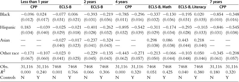
The dependent variable is the mental composite score, which is normalized to have a mean of zero and a standard deviation of one in each wave for the full, unweighted sample in CPP and the full sample with wave 3 weights in ECLS-B. Non-Hispanic whites are the omitted race category in each regression and all race coefficients are relative to that group. The unit of observation is a child. Estimation is done using weighted least squares for the ECLS-B sample (columns 3–6 and 9–12) using sample weights provided in the third wave of the data set. Estimation is done using ordinary least squares for the CPP sample (columns 1–2, 7–8, and 13–14). In addition to the variables included in the table, indicator variables for children with missing values on each covariate are also included in the regressions. Standard errors are in parentheses. Columns 1 through 4 present results for children under one year; Columns 5 and 6 present results for 2-year-olds; Columns 7 through 12 present results for 4-year-olds; Columns 13 and 14 present results for 7-year-olds.
In infancy, blacks lag whites by 0.077 (0.031) standard deviations in the raw ECLS-B data. Hispanics and Asians also slightly trail whites by 0.025 (0.029) and 0.027 (0.040), respectively. Adding our set of controls eliminates these trivial differences. The patterns in the CPP data are strikingly similar. Yet, raw gaps of almost 0.4 standard deviations between blacks and whites are present on the test of mental function in the ECLS-B at age two. Even after including extensive controls, a black-white gap of 0.219 (0.036) standard deviations remains. Hispanics look similar to blacks. Asians lag whites by a smaller margin than blacks or Hispanics in the raw data but after including controls they are the worst-performing ethnic group. By age four, a large test score gap has emerged for blacks and Hispanics in both datasets—but especially in the CPP. In the raw CPP data, blacks lag whites by almost 0.8 standard deviations and Hispanics fare even worse. The inclusion of controls reduces the gap to roughly 0.3 standard deviations for blacks and 0.5 standard deviations for Hispanics. In the ECLS-B, black math scores trail white scores by 0.337 (0.032) in the raw data and trail by 0.130 (0.036) with controls. Black-white differences in literacy are −0.195 (0.031) without controls and 0.020 (0.035) with controls. The identical estimates for Hispanics are −0.311 (0.029) and −0.174 (0.034) in math; −0.293 (0.028) and −0.103 (0.033) in literacy. Asians are the highest-performing ethnic group in both subjects on the age four tests. Racial disparities at age seven, available only in CPP, are generally similar to those at age four.
There are at least three possible explanations for the emergence of racial differences with age. The first is that the skills tested in one-year-olds are not the same as those required of older children, and there are innate racial differences only in the skills that are acquired later. For instance, an infant scores high if she babbles expressively or looks around to find the source of the noise when a bell rings, while older children are tested directly on verbal skills and puzzle-solving ability. Despite these clear differences in the particular tasks undertaken, the outcomes of these early and subsequent tests are correlated by about 0.30, suggesting that they are, to some degree, measuring a persistent aspect of a child’s ability.23 Also relevant is the fact that the Bayley Scales of Infant Development (BSID) score is nearly as highly correlated with measures of parental IQ as childhood aptitude tests.
Racial differences in rates of development are a second possible explanation for the patterns in our data. If black infants mature earlier than whites, then black performance on early tests may be artificially inflated relative to their long-term levels. On the other hand, if blacks are less likely to be cognitively stimulated at home or more likely to be reared in environments that Shonkoff (2006) would label as characterized by “toxic stress,” disruptions in brain development may occur, which may significantly retard cognitive growth.
A third possible explanation for the emerging pattern of racial gaps is that the relative importance of genes and environmental factors in determining test outcomes varies over time. In contrast to the first two explanations mentioned above, under this interpretation, the measured differences in test scores are real, and the challenge is to construct a model that can explain the racial divergence in test scores with age.
To better understand the third explanation, Fryer and Levitt (forthcoming) provide two statistical models that are consistent with the data presented above. Here we provide a briefoverview of the models and their predictions.
The first parameter of interest is the correlation between test scores early on and later in life. Fryer and Levitt (forthcoming) assign a value of 0.30 to that correlation. The measured correlation between test scores early and late in life and parental test scores is also necessary for the analysis. Based on prior research (e.g., Yeates et al., 1983), we take these two correlations as 0.36 and 0.39, respectively.24 The estimated black-white test score gap at young ages is taken as 0.077 based on our findings in ECLS-B, compared to a gap of 0.78 at later ages based on our findings in CPP.
The primary puzzle raised by our results is the following: how does one explain small racial gaps on the BSID test scores administered at ages 8 to 12 months and large racial gaps in tests of mental ability later in life, despite the fact that these two test scores are reasonably highly correlated with one another (ρ = 0.3), and both test scores are similarly correlated with parental test scores (ρ ≥ 0.3)?
The basic building blocks
Let θa denote the measured test score of an individual at age a. We assume that test scores are influenced by an individual’s genetic make-up (G) and his environment (Ea) at age a. The simplest version of the canonical model of genes and environment takes the following form:
![]() (3)
(3)
In this model, the individual’s genetic endowment is fixed over time, but environmental factors vary and their influence may vary. θa, G, and Ea are all normalized into standard deviation units. Initially we will assume that G, Ea, and ∈a are uncorrelated for an individual at any point in time (this assumption will be relaxed below), and that Ea and the error terms for an individual at different ages are also uncorrelated.25 There will, however, be a positive correlation between an individual’s genetic endowment G and the genetic endowment of his or her mother (which we denote Gm). We will further assume, in accord with the simplest models of genetic transmission, that the correlation between G and Gm is 0.50.26
We are interested in matching two different aspects of the data: (1) correlations between test scores, and (2) racial test score gaps at different ages. The test score correlations of interest are those of an individual at the age of one (for which we use the subscript b for baby) and later in childhood (denoted with subscript c).
Under the assumptions above, these correlations are as follows:
![]() (4)
(4)
![]() (5)
(5)
![]() (6)
(6)
where the 0.5 in the first two equations reflects the assumed genetic correlation between mother and child, and the values 0.36, 0.39, and 0.30 are our best estimates of the empirical values of these correlations based on past research cited above.
The racial test score gaps in this model are given by:
![]() (7)
(7)
![]() (8)
(8)
where the symbol Δ in front of a variable signifies the mean racial gap between blacks and whites for that variable. The values 0.077 and 0.854 represent our estimates of the black-white test score gap at ages nine months and seven years from Table 5.27 For Hispanics, these differences are 0.025 and 0.846, respectively.
Solving Eqs (4)–(6), this simple model yields a value of 1.87 for ![]() . Under the assumptions of the model, however, the squared value of the coefficients α and β represent the share of the variance in the measured test score explained by genetic and environmental factors, respectively, meaning that
. Under the assumptions of the model, however, the squared value of the coefficients α and β represent the share of the variance in the measured test score explained by genetic and environmental factors, respectively, meaning that ![]() is bounded at one. Thus, this simple model is not consistent with the observed correlations in the data. The correlation between child and mother test scores observed in the data is too large relative to the correlation between the child’s own test scores at different ages.
is bounded at one. Thus, this simple model is not consistent with the observed correlations in the data. The correlation between child and mother test scores observed in the data is too large relative to the correlation between the child’s own test scores at different ages.
Consequently, we consider two extensions to this simple model that can reproduce these correlations in the data: assortative mating and allowing for a mother’s test score to influence the child’s environment.28
Assortative mating
If women with high G mate with men who also have high G, then the parent child corr(G, Gm) is likely to exceed 0.50. Assuming a value of am = 0.80, which is consistent with prior research, the necessary corr(G, Gm) to solve the system of equations above is roughly 0.76, which requires the correlation between parents on G to be around 0.50, not far from the 0.45 value reported for that coefficient in a literature review (Jensen, 1978).29 With that degree of assortative mating, the other parameters that emerge from the model are αb = 0.53 and αc = 0.57. Using these values of ab and ac, it is possible to generate the observed racial gaps in (7) and (8). If we assume as an upper bound that environments for black and Hispanic babies are the same as those for white babies (i.e., ΔEb = 0) in Eq. (7), then the implied racial gap in G is a modest 0.145 standard deviations for blacks and 0.04 for Hispanics.30
To fit Eq. (8) requires βcΔEc = 0.77. If βc = 0.77 (implying that environmental factors explain about half of the variance in test scores), then a one standard deviation gap in environment between black and white children and a 1.14 standard deviation gap between Hispanic and white children would be needed to generate the observed childhood racial test score gap31. If environmental factors explain less of the variance, a larger racial gap in environment would be needed. Taking a simple non-weighted average across environmental proxies available in the ECLS yields a 1.2 standard deviation gap between blacks and whites32.
Allowing parental test scores to influence the child’s environment
A second class of model consistent with our empirical findings is one in which the child’s environment is influenced by the parent’s test score, as in Dickens and Flynn (2001). One example of such a model would be
![]() (9)
(9)
where Eq. (9) differs from the original Eq. (3) by allowing the child’s environment to be a function of the mother’s test score, as well as factors ![]() that are uncorrelated with the mother’s test score. In addition, we relax the earlier assumption that the environments an individual experiences as a baby and as a child are uncorrelated. We do not, however, allow for assortative mating in this model. Under these assumptions, Eq. (9) produces the following three equations for our three key test score correlations
that are uncorrelated with the mother’s test score. In addition, we relax the earlier assumption that the environments an individual experiences as a baby and as a child are uncorrelated. We do not, however, allow for assortative mating in this model. Under these assumptions, Eq. (9) produces the following three equations for our three key test score correlations
![]() (10)
(10)
![]() (11)
(11)
![]() (12)
(12)
Allowing parental ability to influence the child’s environment introduces extra degrees of freedom; indeed, this model is so flexible that it can match the data both under the assumption of very small and large racial differences in G (e.g., ΔG ≤ 1 standard deviation). In order for our findings to be consistent with small racial differences in G, the importance of environmental factors must start low and grow sharply with age. In the most extreme case (where environment has no influence early in life: βb = 0), solving Eqs (10) and (12) implies αb = 0.80 and αc = 0.37. If βc = 0.77 (as in the assortative mating model discussed above), then a correlation of 0.29 between the mother’s test score and the child’s environment is necessary to solve Eq. (11). The mean racial gap in G implied by Eq. (7) is 0.096 standard deviations. To match the test score gap for children requires a mean racial difference in environmental factors of approximately one standard deviation.
A model in which parents’ scores influence their offspring’s environment is, however, equally consistent with mean racial gaps in G of one standard deviation. For this to occur, G must exert little influence on the baby’s test score, but be an important determinant of the test scores of children. Take the most extreme case in which G has no influence on the baby’s score (i.e., αb = 0). If genetic factors are not directly determining the baby’s test outcomes, then environmental factors must be important. Assuming βb = 0.80, Eq. (10) implies a correlation between the mother’s test score and the baby’s environment of 0.45. If we assume that the correlation between the baby’s environment and the child’s environment is 0.70, then Eq. (12) implies a value of βc = 0.54. If we maintain the earlier assumption of ![]() = 0.80, as well as a correlation between the mother’s test score and the child’s environment of 0.32, then a value of αc = 0.49 is required to close the model. If there is a racial gap of one standard deviation in G, then Eqs (7) and (8) imply 0.096 and 0.67 standard deviation racial gaps in environment factors for babies and children, respectively, to fit our data.
= 0.80, as well as a correlation between the mother’s test score and the child’s environment of 0.32, then a value of αc = 0.49 is required to close the model. If there is a racial gap of one standard deviation in G, then Eqs (7) and (8) imply 0.096 and 0.67 standard deviation racial gaps in environment factors for babies and children, respectively, to fit our data.
Putting the pieces together, the above analysis shows that the simplest genetic models are not consistent with the evidence presented on racial differences in the cognitive ability of infants. These inconsistencies can be resolved in two ways: incorporating assortative mating or allowing parental ability to affect the offspring’s environment. With assortative mating, our data imply a minimal racial gap in intelligence (0.11 standard deviations as an upper bound), but a large racial gap in environmental factors. When parent’s ability influences the child’s environment, our results can be made consistent with almost any value for a racial gap in G (from roughly zero to a full standard deviation), depending on the other assumptions that are made. Thus, despite stark empirical findings, our data cannot resolve these difficult questions—much depends on the underlying model.
4 Interventions to foster human capital before children enter school
In the past five decades there have been many attempts to close the racial achievement gap before kids enter school.33 Table 6 provides an overview of twenty well-known programs, the ages they serve, and their treatment effects (in the cases in which they have been credibly evaluated).
Table 6
Early childhood interventions to increase achievement.
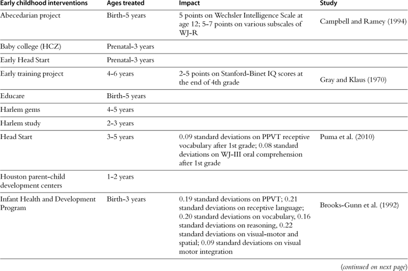

The set of interventions included in this table was generated in two ways. First, we used Heckman (1999) and Heckman et al. (2009) as the basis for a thorough literature review on early childhood intervention programs. We investigated all of the programs included in these papers, and then examined the papers written on this list of programs for additional programs. Second, we examined all of the relevant reports available through the IES What Works Clearinghouse. From this original list, we included twenty of the most credibly evaluated, largest scale programs in our final list.
Perhaps the most famous early intervention program for children involved 64 students in Ypsilanti, Michigan, who attended the Perry Preschool program in 1962. The program consisted of a 2.5-hour daily preschool program and weekly home visits by teachers, and targeted children from disadvantaged socioeconomic backgrounds with IQ scores in the range of 70–85. An active learning curriculum—High/Scope—was used in the preschool program in order to support both the cognitive and non-cognitive development of the children over the course of two years beginning when the children were three years old. Schweinhart et al. (1993) find that students in the Perry Preschool program had higher test scores between the ages of 5 and 27, 21% less grade retention or special services required, 21% higher graduation rates, and halfthe number of lifetime arrests in comparison to children in the control group. Considering the financial benefits that are associated with the positive outcomes of the Perry Preschool, Heckman et al. (2009) estimated that the rate of return on the program is between 7 and 10%, passing a cost-benefit analysis.
Another important intervention, which was initiated three years after the Perry Preschool program is Head Start. Head Start is a preschool program funded by federal matching grants that is designed to serve 3- to 5-year-old children living at or below the federal poverty level.34 The program varies across states in terms of the scope of services provided, with some centers providing full-day programs and others only half-day. In 2007, Head Start served over 900,000 children at an average annual cost of about $7300 per child.
Evaluations of Head Start have often been difficult to perform due to the non-random nature of enrollment in the program. Currie and Thomas (1995) use a national sample of children and compare children who attended a Head Start program with siblings who did not attend Head Start, based on the assumption that examining effects within the family unit will reduce selection bias. They find that those children who attended Head Start scored higher on preschool vocabulary tests but that for black students, these gains were lost by age ten. Using the same analysis method with updated data, Garces et al. (2002) find several positive outcomes associated with Head Start attendance. They conclude that there is a positive effect from Head Start on the probability of attending college and—for whites—the probability of graduating from high school. For black children, Head Start led to a lower likelihood of being arrested or charged with a crime later in life.
Puma et al. (2005), in response to the 1998 reauthorization of Head Start, conduct an evaluation using randomized admission into Head Start.35 The impact of being offered admission into Head Start for three and four year olds is 0.10 to 0.34 standard deviations in the areas of early language and literacy. For 3-year-olds, there were also small positive effects in the social-emotional domain (0.13 to 0.18 standard deviations) and on overall health status (0.12 standard deviations). Yet, by the time the children who received Head Start services have completed first grade, almost all of the positive impact on initial school readiness has faded. The only remaining impacts in the cognitive domain are a 0.08 standard deviation increase in oral comprehension for 3-year-old participants and a 0.09 standard deviation increase in receptive vocabulary for the 4-year-old cohort (Puma et al., 2010).36
A third, and categorically different, program is the Nurse Family Partnership. Through this program, low-income first-time mothers receive home visits from a registered nurse beginning early in the pregnancy that continue until the child is two years old—a total of fifty visits over the first two years. The program aims to encourage preventive health practices, reduce risky health behaviors, foster positive parenting practices, and improve the economic self-sufficiency of the family. In a study of the program in Denver in 1994–95, Olds et al. (2002) find that those children whose mothers had received home visits from nurses (but not those who received home visits from paraprofessionals) were less likely to display language delays and had superior mental development at age two. In a long-term evaluation of the program, Olds et al. (1998) find that children born to women who received nurse home visits during their pregnancy between 1978 and 1980 have fewer juvenile arrests, convictions, and violations of probation by age fifteen than those whose mothers did not receive treatment.
Other early childhood interventions—many based on the early success of the Perry Preschool, Head Start, and the Nurse Family Partnership—include the Abecedarian Project, the Early Training Project, the Infant Health and Development Program, the Milwaukee Project, and Tulsa’s universal pre-kindergarten program. The Abecedarian Project provided full-time, high-quality center-based childcare services for four cohorts of children from low-income families from infancy through age five between 1971 and 1977. Campbell and Ramey (1994) find that at age twelve, those children who were randomly assigned to the project scored 5 points higher on the Wechsler Intelligence Scale and 5–7 points higher on various subscales of the Woodcock-Johnson Psycho-Educational Battery achievement test. The Early Training Project provided children from low-income homes with summertime experiences and weekly home visits during the three summers before entering first grade in an attempt to improve the children’s school readiness. Gray and Klaus (1970) report that children who received these intervention services maintained higher Stanford-Binet IQ scores (2–5 points) at the end of fourth grade. The Infant Health and Development Program specifically targeted families with low birthweight, preterm infants and provided them with weekly home visits during the child’s first year and biweekly visits through age three, as well as enhanced early childhood educational care and bimonthly parent group meetings. Brooks-Gunn et al. (1992) report that this program had positive effects on language development at the end of first grade, with participant children scoring 0.09 standard deviations higher on receptive vocabulary and 0.08 standard deviations higher on oral comprehension. The Milwaukee Project targeted newborns born to women with IQs lower than 80; mothers received education, vocational rehabilitation, and child care training while their children received high-quality educational programming and three balanced meals daily at “infant stimulation centers” for seven hours a day, five days a week until the children were six years old. Garber (1988) finds that this program resulted in an increase of 23 points on the Stanford-Binet IQ test at age six for treatment children compared to control children.
Unlike the other programs described, Tulsa’s preschool program is open to all 4-year-old children. It is a basic preschool program that has high standards for teacher qualification (a college degree and early childhood certification are both required) and a comparatively high rate of penetration (63% of eligible children are served). Gormley et al. (2005) use a birthday cutoff regression discontinuity design to evaluate the program and find that participation improves scores on the Woodcock-Johnson achievement test significantly (from 0.38 to 0.79 standard deviations).
Beyond these highly effective programs, Table 6 demonstrates that there is large variance in the effectiveness of well-known early childhood programs. The Parents as Teachers Program, for instance, shows mixed and generally insignificant effects on initial measures of cognitive development (Wagner and Clayton, 1999). In an evaluation of the Houston Parent-Child Development Centers, Andrews et al. (1982) find no significant impact on children’s cognitive skills at age one and mixed impacts on cognitive development at age two. Even so, the typical early childhood intervention passes a simple cost-benefit analysis.37
There are two potentially important caveats going forward. First, most of the programs are built on the insights gained from Perry and Head Start, yet what we know about infant development in the past five decades has increased dramatically. For example, psychologists used to assume that there was a relatively equal degree of early attachment across children but they now acknowledge that there is a great deal of variance in the stability of early attachment (Thompson, 2000). Tying new programs to the lessons learned from previously successful programs while incorporating new insights from biology and developmental psychology is both the challenge and opportunity going forward.
Second, and more important for our purposes here, even the most successful early interventions cannot close the achievement gap in isolation. If we truly want to eliminate the racial achievement gap, early interventions may or may not be necessary but the evidence forces one to conclude that they are not sufficient.
5 The racial achievement gap in kindergarten through 12th grade
As we have seen, children begin life on equal footing, but important differences emerge by age two and their paths quickly diverge. In this section, we describe basic facts about the racial achievement gap from the time children enter kindergarten to the time they exit high school. Horace Mann famously argued that schools were “the great equalizer,” designed to eliminate differences between children that are present when they enter school because of different background characteristics. As this section will show, if anything, schools currently tend to exacerbate group differences.
Basic facts about racial differences in educational achievement using ECLS-K
The Early Childhood Longitudinal Study, Kindergarten Cohort (ECLS-K) is a nationally representative sample of over 20,000 children entering kindergarten in 1998. Information on these children has been gathered at six separate points in time. The full sample was interviewed in the fall and spring of kindergarten, and the spring of first, third, fifth, and eighth grades. Roughly 1000 schools are included in the sample, with an average of more than twenty children per school in the study. As a consequence, it is possible to conduct within-school or even within-teacher analyses.
A wide range of data is gathered on the children in the study, which is described in detail at the ECLS website http://nces.ed.gov/ecls. We utilize just a small subset of the available information in our baseline specifications, the most important of which are cognitive assessments administered in kindergarten, first, third, fifth, and eighth grades. The tests were developed especially for the ECLS, but are based on existing instruments including Children’s Cognitive Battery (CCB); Peabody Individual Assessment Test—Revised (PIAT-R); Peabody Picture Vocabulary Test-3 (PPVT-3); Primary Test of Cognitive Skills (PTCS); and Woodcock-Johnson Psycho-Educational Battery—Revised (WJ-R). The questions are administered orally through spring of first grade, as it is not assumed that students know how to read until then. Students who are missing data on test scores, race, or gender are dropped from our sample. Summary statistics for the variables we use in our core specifications are displayed by race in Table A.6.
Table 7 presents a series of estimates of the racial test score gap in math (Panel A) and reading (Panel B) for the tests taken over the first nine years of school. Similar to our analysis of younger children in the previous section, the specifications estimated are least squares regressions of the form:
Table 7
The evolution of the achievement gap (ECLS), K-8.
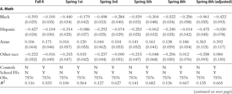
The dependent variable in each column is test score from the designated subject and grade. Odd-numbered columns estimate the raw racial test score gaps and do not include any other controls. Specifications in the even-numbered columns include controls for socioeconomic status, number of books in the home (linear and quadratic terms), gender, age, birth weight, dummies for mother’s age at first birth (less than twenty years old and at least thirty years old), a dummy for being a Women, Infants, Children (WIC) participant, missing dummies for all variables with missing data, and school fixed effects. Test scores are IRT scores, normalized to have mean zero and standard deviation one in the full, weighted sample. Non-Hispanic whites are the omitted race category, so all of the race coefficients are gaps relative to that group. The sample is restricted to students from whom data were collected in every wave from fall kindergarten through spring eighth grade, as well as students who have non-missing race and non-missing gender. Panel weights are used. The unit of observation is a student. Robust standard errors are located in parentheses.
![]() (13)
(13)
where outcomei,g denotes an individual i ’s test score in grade g and Xi, represents an array of student-level social and economic variables describing each student’s environment. The variable Ri, is a full set of race dummies included in the regression, with non-Hispanic white as the omitted category. In all instances, we use sampling weights provided in the dataset.
The vector Xi, contains a parsimonious set of controls—the most important of which is a composite measure of socio-economic status constructed by the researchers conducting the ECLS survey. The components used in the SES measure are parental education, parental occupational status, and household income. Other variables included as controls are gender, child’s age at the time of enrollment in kindergarten, WIC participation (a nutrition program aimed at relatively low income mothers and children), mother’s age at first birth, birth weight, and the number of children’s books in the home.38 When there are multiple observations of social and economic variables (SES, number of books in the home, and so on), for all specifications, we only include the value recorded in the fall kindergarten survey.39 While this particular set of covariates might seem idiosyncratic, Fryer and Levitt (2004) have shown that results one obtains with this small set of variables mirror the findings when they include an exhaustive set of over 100 controls. Again, we stress that a causal interpretation is unwarranted; we view these variables as proxies for a broader set of environmental and behavioral factors. The odd-numbered columns of Table 7 present the differences in means, not including any covariates. The even-numbered columns mirror the main specification in Fryer and Levitt (2004).
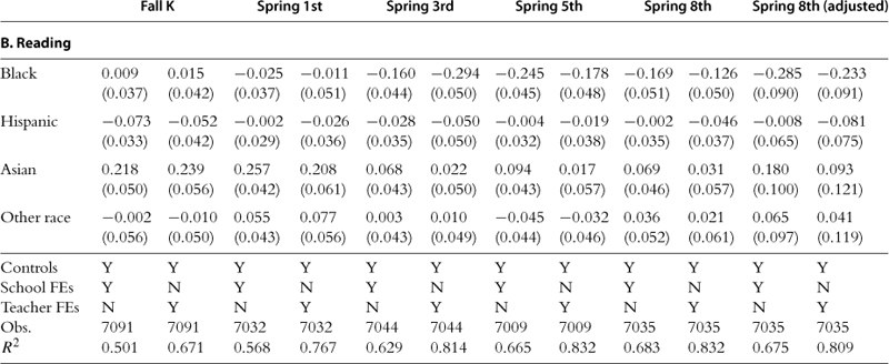
The raw black-white gap in math when kids enter school is 0.393 (0.029), shown in column one of Panel A. Adding our set of controls decreases this difference to 0.100 (0.035). By fifth grade, Asians outperform other racial groups and Hispanics have gained ground relative to whites, but blacks have lost significant ground. The black-white achievement gap in fifth grade is 0.539 (0.033) standard deviations without controls and 0.304 (0.048) with controls. Disparities in eighth grade look similar, but a peculiar aspect of ECLS-K (very similar tests from kindergarten through eighth grade with different weights on the components of the test) masks potentially important differences between groups. If one restricts attention on the eighth grade exam to subsections of the test which are not mastered by everyone (eliminating the counting and shapes subsection, for example), a large racial gap emerges. Specifically, blacks are trailing whites by 0.961 (0.055) in the raw data and 0.422 (0.093) with the inclusion of controls.
The black-white test score gap grows, on average, roughly 0.60 standard deviations in the raw data and 0.30 when we include controls between the fall of kindergarten and spring of eighth grade. The table also illustrates that the control variables included in the specification shrink the gap a roughly constant amount of approximately 0.30 standard deviations regardless of the year of testing. In other words, although blacks systematically differ from whites on these background characteristics, the impact of these variables on test scores is remarkably stable over time. Whatever factor is causing blacks to lose ground is likely operating through a different channel.40
In contrast to blacks, Hispanics gain substantial ground relative to whites, despite the fact that they are plagued with many of the social problems that exist among blacks— low socioeconomic status, inferior schools, and so on. One explanation for Hispanic convergence is an increase in English proficiency, though we have little direct evidence on this question.41 Calling into question that hypothesis is the fact that after controlling for other factors Hispanics do not test particularly poorly on reading, even upon school entry. Controlling for whether or not English is spoken in the home does little to affect the initial gap or the trajectory of Hispanics.42 The large advantage enjoyed by Asians in the first two years of school is maintained. We also observe striking losses by girls relative to boys in math—over two-tenths of a standard deviation over the four-year period— which is consistent with other research (Becker and Forsyth, 1994; Fryer and Levitt, forthcoming).
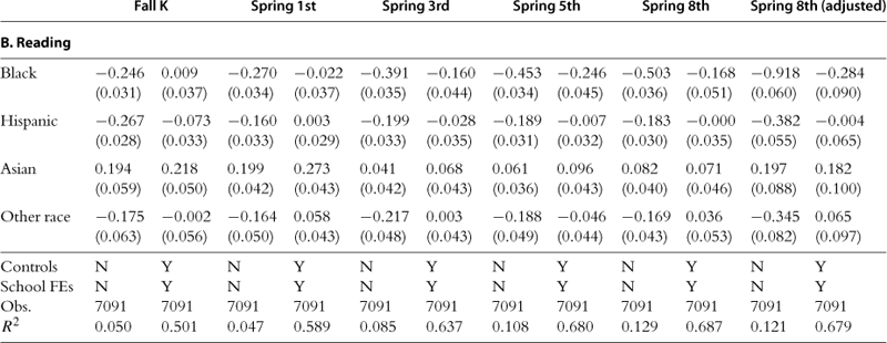
Panel B of Table 7 is identical to Panel A, but estimates racial differences in reading scores rather than math achievement. After adding our controls, black children score very similarly to whites in reading in the fall of kindergarten. As in math, however, blacks lose substantial ground relative to other racial groups over the first nine years of school. The coefficient on the indicator variable black is 0.009 standard deviations above whites in the fall of kindergarten and 0.246 standard deviations below whites in the spring of fifth grade, or a loss of over 0.25 standard deviations for the typical black child relative to the typical white child. In eighth grade, the gap seems to shrink to 0.168 (0.051), but accounting for the fact that a large fraction of students master the most basic parts of the exam left over from the early elementary years gives a raw gap of 0.918 (0.060) and 0.284 (0.090) with controls. The impact of covariates—explaining about 0.2 to 0.25 of a standard deviation gap between blacks and whites across most grades—is slightly smaller than in the math regressions. Hispanics experience a much smaller gap relative to whites, and it does not grow over time. The early edge enjoyed by Asians diminishes by third grade.
One potential explanation for such large racial achievement gaps, even after accounting for differences in the schools that racial minorities attend, is the possibility that they are assigned inferior teachers within schools. If whites and Asians are more likely to be in advanced classes with more skilled teachers then this sorting could exacerbate differences and explain the divergence over time. Moreover, with such an intense focus on teacher quality as a remedy for racial achievement gaps, it useful to understand whether and the extent to which gaps exist when minorities and non-minorities have the same teacher. This analysis is possible in ECLS-K—the data contain, on average, 3.3 students per teacher within each year of data collection (note that because the ECLS surveys subsamples within each classroom, this does not reflect the true student-teacher ratios in these classrooms).
Table 8 estimates the racial achievement gap in math and reading over the first nine years of school including teacher fixed effects. For each grade, there are two columns. The first column estimates racial differences with school fixed effects on a sample of students for whom we have valid information on their teacher. This restriction reduces the sample approximately one percent from the original sample in Table 7. Across all grades and both subjects, accounting for sorting into classrooms has very little marginal impact on the racial achievement gap beyond including school fixed effects. The average gain in standard deviations from including teacher fixed effects is only about 0.014. The minimum marginal gain from including the teacher controls is 0.006 and the maximum difference is 0.072; however, in several cases the gap is not actually reduced by including teacher fixed effects. There are two important takeaways. First, differential sorting within schools does not seem to be an important contributor to the racial achievement gap. Second, although much has been made of the importance of teacher quality in eliminating racial disparities (Levin and Quinn, 2003; Barton, 2003), the above analysis suggests that racial gaps among students with the same teacher are stark.
Table 8
The evolution of the achievement gap (ECLS), K-8: accounting for teachers.
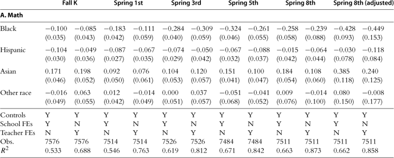
The dependent variable in each column is test score from the designated subject and grade. All specifications include controls for race, socioeconomic status, number of books in the home (linear and quadratic terms), gender, age, birth weight, dummies for mother’s age at first birth (less than twenty years old and at least thirty years old), a dummy for being a Women, Infants, Children (WIC) participant, and missing dummies for all variables with missing data. Odd-numbered columns include school fixed effects, whereas even-numbered columns include teacher fixed effects. Test scores are IRT scores, normalized to have mean zero and standard deviation one in the full, weighted sample. Non-Hispanic whites are the omitted race category, so all of the race coefficients are gaps relative to that group. The sample is restricted to students from whom data were collected in every wave from fall kindergarten through spring eighth grade and students for whom teacher data was available in the relevant grade, as well as students who have non-missing race and non-missing gender. Panel weights are used. The unit of observation is a student. Robust standard errors are located in parentheses.
In an effort to uncover the factors that are associated with the divergent trajectories of blacks and whites, Table 9 explores the sensitivity of these “losing ground” estimates across a wide variety of subsamples of the data. We report only the coefficients on the black indicator variable and associated standard errors in the table. The top row of the table presents the baseline results using a full sample and our parsimonious set of controls (the full set of controls used in Tables 7 and 8, but omitting fixed effects). For the eighth grade scores, we restrict the test to components that are not mastered by all students.43 In that specification, blacks lose an average of 0.356 (0.047) standard deviations in math and 0.483 (0.060) in reading relative to whites over the first nine years of school.
Table 9
Sensitivity analysis for losing ground, ECLS (Fall K vs. Spring 8th).
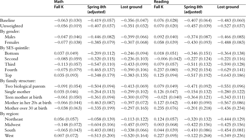

Specifications in this table include controls for race, socioeconomic status, number of books in the home (linear and quadratic terms), gender, age, birth weight, dummies for mother’s age at first birth (less than twenty years old and at least thirty years old), a dummy for being a Women, Infants, Children (WIC) participant, and missing dummies for all variables with missing data. Only the coefficients on black are reported. The sample is restricted to students from whom data were collected in every wave from fall kindergarten through spring eighth grade, as well as students who have non-missing race and non-missing gender. Panel weights are used (except in the specification). The top row shows results from the baseline specification across the entire sample, the second row shows the results when panel weights are omitted, and the remaining rows correspond to the baseline specification restricted to particular subsets of the data.
Surprisingly, blacks lose similar amounts of ground across many subsets of the data, including by sex, location type, and whether or not a student attends private schools. The results vary quite a bit across the racial composition of schools, quintiles of the socioeconomic status distribution, and by family structure. Blacks in schools with greater than fifty percent blacks lose substantially more ground in math than do blacks in greater than fifty percent white schools. In reading, their divergence follows similar paths. The top three SES quintiles lose more ground than the lower two quintiles in both math and reading, but the differences are particularly stark in reading. The two largest losing ground coefficients in the table are for the fourth and fifth quintile of SES in reading. Black students in these categories lose ground at an alarming rate—roughly 0.6 standard deviations over 9 years. This latter result could be related to the fact that, in the ECLS-K, a host of variables which are broad proxies for parenting practices differ between blacks and whites. For instance, black college graduates have the same number of children’s books for their kids as white high school graduates. A similar phenomenon emerges with respect to family structure; the most ground is lost, relative to whites, by black students who have both biological parents. Investigating within-race regressions, Fryer and Levitt (2004) show that the partial correlation between SES and test scores are about half the magnitude for blacks relative to whites. In other words, there is something that higher income buys whites that is not fully realized among blacks. The limitation of this argument is that including these variables as controls does not substantially alter the divergence in black-white achievement over the first nine years of school. This issue is beyond the scope of this chapter but deserves further exploration.
We conclude our analysis of ECLS-K by investigating racial achievement gaps on questions assessing specific skills in kindergarten and eighth grade. Table 10 contains unadjusted means on questions tested in each subsample of the test. The entries in the table are means of probabilities that students have mastered the material in that subtest. Math sections include: counting, numbers, and shapes; relative size; ordinality and sequence; adding and subtracting; multiplying and dividing; place value; rate and measurement; fractions; and area and volume. Reading sections include: letter recognition, beginning sounds, ending sounds, sight words, words in context, literal inference, extrapolation, evaluation, nonfiction evaluation, and complex syntax evaluation. In kindergarten, the test excluded fractions and area and volume (in math) as well as nonfiction evaluation and complex syntax evaluation (in reading).
Table 10
Unadjusted means on questions assessing specific sets of skills, ECLS.
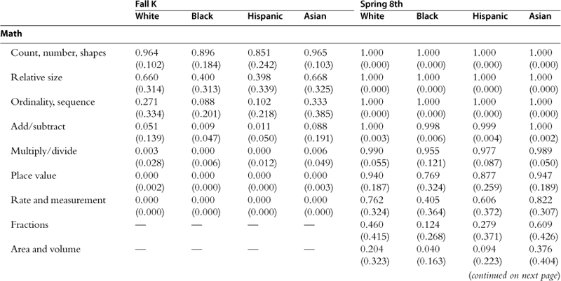
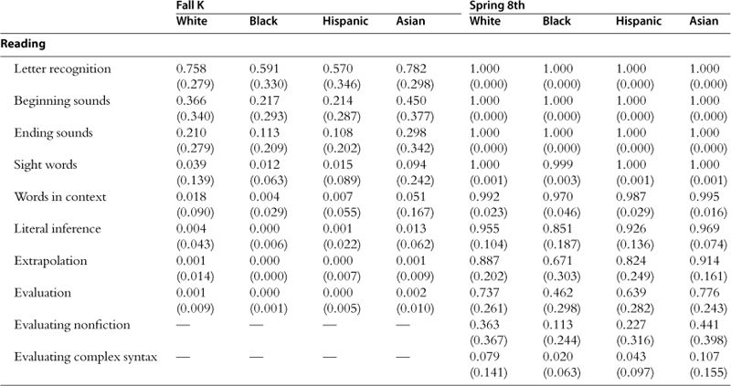
Entries are unadjusted mean scores on specific areas of questions in kindergarten fall and eighth grade spring. They are proficient probability scores, which are constructed using IRT scores and provide the probability of mastery of a specific set of skills. Dashes indicate areas that were not included in kindergarten fall exams. Standard deviations are located in parentheses.
All students enter kindergarten with a basic understanding of counting, numbers, and shapes. Black students have a probability of 0.896 (0.184) of having mastered this material and the corresponding probability for whites is 0.964 (0.102). Whites outpace blacks on all other dimensions. Hispanics are also outpaced by whites on all dimensions, while Asians actually fare better than whites on all dimensions. By eighth grade, students have essentially mastered six out of the nine areas tested in math, and six out of the ten in reading. Interestingly, on every dimension where there is room for growth, whites outpace blacks—and by roughly a constant amount. Blacks only begin to close the gap after white students have demonstrated mastery of a specific area and therefore can improve no more. While it is possible that this implies that blacks will master the same material as whites but on a longer timeline, there is a more disconcerting possibility—as skills become more difficult, a non-trivial fraction of black students may never master the skills. If these skills are inputs into future subject matter, then this could lead to an increasing black-white achievement gap. The same may apply to Hispanic children, although they are closer to closing the gap with white students than blacks are.
In summary, using the ECLS-K—a recent and remarkably rich nationally representative dataset of students from the beginning of kindergarten through their eighth grade year—we demonstrate an important and remarkably robust racial achievement gap that seems to grow as children age. Blacks underperform whites in the same schools, the same classrooms, and on every aspect of each cognitive assessment. Hispanics follow a similar, though less stark, pattern.
Basic facts about racial differences in educational achievement using CNLSY79
Having exhausted possibilities in the ECLS-K, we now turn to the Children of the National Longitudinal Survey of Youth 1979 (CNLSY79). The CNLSY79 is a survey of children born to NLSY79 female respondents that began in 1986. The children of these female respondents are estimated to represent over 90% of all the children ever to be born to this cohort of women. As of 2006, a total of 11,466 children have been identified as having been born to the original 6283 NLSY79 female respondents, mostly during years in which they were interviewed. In addition to all the mother’s information from the NLSY79, the child survey includes assessments of each child as well as additional demographic and development information collected from either the mother or child. The CNLSY79 includes the Home Observation for Measurement of Environment (HOME), an inventory of measures related to the quality of the home environment, as well as three subtests from the full Peabody Individual Achievement Test (PIAT) battery: the Mathematics, Reading Recognition, and Reading Comprehension assessments. We use the Mathematics and Reading Recognition assessments for our analysis.44
Most children for whom these assessments are available are between the ages of five and fourteen. Administration of the PIAT Mathematics assessment is relatively straightforward. Children enter the assessment at an age-appropriate item (although this is not essential to the scoring) and establish a “basal” by attaining five consecutive correct responses. If no basal is achieved then a basal of “1” is assigned. A “ceiling” is reached when five of seven items are answered incorrectly. The non-normalized raw score is equivalent to the ceiling item minus the number of incorrect responses between the basal and the ceiling scores. The PIAT Reading Recognition subtest measures word recognition and pronunciation ability, essential components of reading achievement. Children read a word silently, then say it aloud. PIAT Reading Recognition contains 84 items, each with four options, which increase in difficulty from preschool to high school levels. Skills assessed include matching letters, naming names, and reading single words aloud. Table A.7 contains summary statistics for variables used in our analysis.
To our knowledge, the CNLSY is the only large nationally representative sample that contains achievement tests both for mothers and their children, allowing one to control for maternal academic achievement in investigating racial disparities in achievement. Beyond the simple transmission of any genetic component of achievement, more educated mothers are more likely to spend time with their children engaging in achievement-enhancing activities such as reading, using academically stimulating toys, encouraging young children to learn the alphabet and numbers, and so on (Klebanov, 1994).
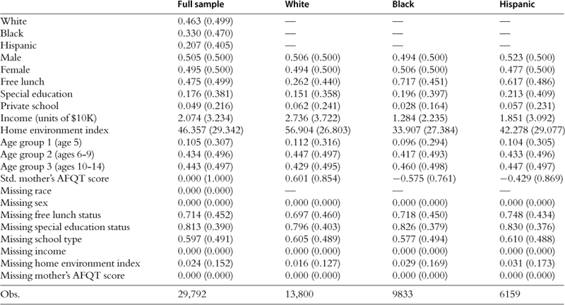
Tables 11 and 12 provide estimates of the racial achievement gap, by age, for children between the ages of five and fourteen.45 Table 11 provides estimates for elementary school ages and Table 12 provides similar estimates for middle school aged children. Both tables contain two panels: Panel A presents results for math achievement and Panel B presents results for reading achievement. The first column under each age presents raw racial differences (and includes dummies for the child’s age in months and for the year in which the assessment was administered). The second column adds controls for race, gender, free lunch status, special education status, whether the child attends a private school, family income, the HOME inventory, mother’s standardized AFQT score, and dummies for the mother’s birth year. Most important of these controls, and unique relative to other datasets, is maternal AFQT.
Table 11
Determinants of PIAT math and reading recognition scores, elementary school (CNLSY79).
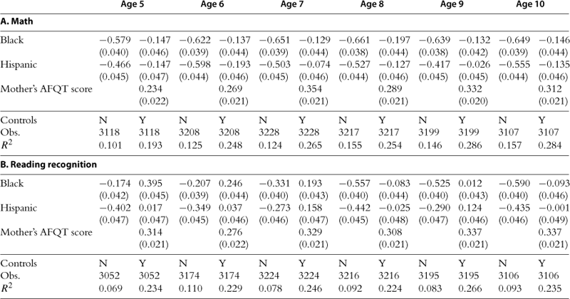
The dependent variable in each column is the Peabody Individual Achievement Test (PIAT) score for the designated subject and age. All specifications include dummies for the child’s age in months and dummies for the year in which the assessment was administered. Odd-numbered columns estimate the raw racial test score gaps and also include a dummy for missing race. Non-black, non-Hispanic respondents are the omitted race category, so all of the race coefficients are gaps relative to that group. Specifications in the even-numbered columns include controls for gender, free lunch status, special education status, a dummy for attending a private school, parents’ income, the Home Observation for Measurement of Environment (HOME) inventory, which is an inventory of measures related to the quality of the home environment, mother’s AFQT score (standardized across the entire sample of mothers in our dataset), and dummies for the mother’s birth year. Also included are missing dummies for all variables with missing data. Robust standard errors are located in parentheses. See data appendix for details of the sample construction.
Table 12
Determinants of PIAT math and reading recognition scores, middle school (CNLSY79).
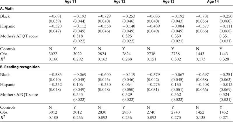
The dependent variable in each column is the Peabody Individual Achievement Test (PIAT) score for the designated subject and age. All specifications include dummies for the child’s age in months and dummies for the year in which the assessment was administered. Odd-numbered columns estimate the raw racial test score gaps and also include a dummy for missing race. Non-black, non-Hispanic respondents are the omitted race category, so all of the race coefficients are gaps relative to that group. Specifications in the even-numbered columns include controls for gender, free lunch status, special education status, a dummy for attending a private school, parents’ income, the Home Observation for Measurement of Environment (HOME) inventory, which is an inventory of measures related to the quality of the home environment, mother’s AFQT score (standardized across the entire sample of mothers in our dataset), and dummies for the mother’s birth year. Also included are missing dummies for all variables with missing data. Robust standard errors are located in parentheses. See data appendix for details regarding sample construction.
Two interesting observations emerge. First, gaps in reading are large and positive for blacks relative to whites for children under the age of seven. At age five, blacks are 0.174 (0.042) standard deviations behind whites. Controlling for maternal IQ, blacks are 0.395 (0.045) standard deviations ahead of whites. The black advantage, after controlling for maternal AFQT, tends to decrease as children age. At age fourteen, blacks are one-quarter standard deviation behind whites even after controlling for maternal achievement—a loss of roughly 0.650 standard deviations in ten years.
A second potentially important observation is that, in general, the importance of maternal achievement is remarkably constant over time. Independent of the raw data, maternal achievement demonstrably shifts the black coefficient roughly 0.4 to 0.5 standard deviations relative to whites. At age five, the raw difference between blacks and whites is −0.579 (0.040) in math and −0.174 (0.042) in reading. Accounting for maternal AFQT, these differences are −0.147 (0.046) and 0.395 (0.045)—a 0.432 standard deviation shift in math and 0.569 shift in reading. At age fourteen, maternal achievement explains 0.531 standard deviations in math and 0.446 in reading despite the fact that the raw gaps on both tests increased substantially. The stability of the magnitudes in the shift of the gap once one controls for maternal AFQT suggests that whatever is causing blacks to lose ground relative to whites is operating through a different channel.
Basic facts about racial differences in achievement using district administrative files
Thus far we have concentrated on nationally representative samples because of their obvious advantages. Yet, using the restricted-use version of ECLS-K, we discovered that some large urban areas with significant numbers of chronically underperforming schools may not be adequately represented. For instance, New York City contains roughly 3.84% of black school children, but is only 1.46% of the ECLS-K Sample. Chicago has 2.42% of the population of black students and is only 1.13% of the ECLS-K sample. Ideally, sample weights would correct for this imbalance, but if schools with particular characteristics (i.e., predominantly minority and chronically poor performing) are not sampled or refuse to participate for any reason, weights will not necessarily compensate for this imbalance.
To understand the impact of this potential sampling problem, we collected administrative data from four representative urban school districts: Chicago, Dallas, New York City, and Washington, DC. The richness of the data varies by city, but all data sets include information on student race, gender, free lunch eligibility, behavioral incidents, attendance, matriculation with course grades, whether a student is an English Language Learner (ELL), and special education status. The data also include a student’s first and last names, birth date, and address. We use address data to link every student to their census block group and impute the average income of that block group to every student who lives there. In Dallas and New York we are able to link students to their classroom teachers. New York City administrative files also contain teacher value-added data for teachers in grades four through eight and question-level data for each student’s state assessment.
The main outcome variable in these data is an achievement assessment unique to each city. In May of every school year, students in Dallas public elementary schools take the Texas Assessment of Knowledge and Skills (TAKS) if they are in grades three through eight. New York City administers mathematics and English Language Arts tests, developed by McGraw-Hill, in the winter for students in third through eighth grade. In Washington, DC, the DC Comprehensive Assessment System (DC-CAS) is administered each April to students in grades three through eight and ten. All Chicago students in grades three through eight take the Illinois Standards Achievement Test (ISAT). See the data appendix for more details on each assessment.
One drawback of using school district administrative files is that individual-level controls only include a mutually exclusive and collectively exhaustive set of race dummies, indicators for free lunch eligibility, special education status, and whether a student is an ELL student. A student is income-eligible for free lunch if her family income is below 130% of the federal poverty guidelines, or categorically eligible if (1) the student’s household receives assistance under the Food Stamp Program, the Food Distribution Program on Indian Reservations (FDPIR), or the Temporary Assistance for Needy Families Program (TANF); (2) the student was enrolled in Head Start on the basis of meeting that program’s low-income criteria; (3) the student is homeless; (4) the student is a migrant child; or (5) the student is a runaway child receiving assistance from a program under the Runaway and Homeless Youth Act and is identified by the local educational liaison. Determination of special education and ELL status varies by district. For example, in Washington, DC, special education status is determined through a series of observations, interviews, reviews of report cards and administration of tests. In Dallas, any student who reports that his or her home language is not English is administered a test and ELL status is based on the student’s score. Tables A.8—A.11 provide summary statistics used in our analysis in Chicago, Dallas, New York, and Washington, DC, respectively.
Table 13 presents estimates of the racial achievement gap in math (Panel A) and reading (Panel B) for New York City, Washington, DC, Dallas, and Chicago using the standard least squares specification employed thus far. Each city contains three columns. The first column reports the raw racial gap with no controls. The second column adds a small set of individual controls available in the administrative files in each district and the final column under each city includes school fixed effects.
Table 13
Racial achievement gap in urban districts.
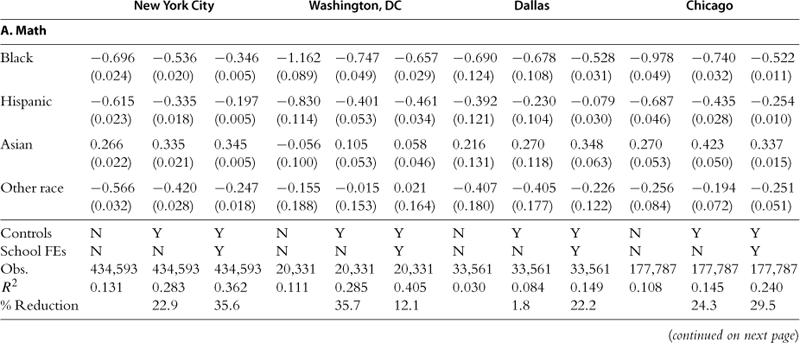
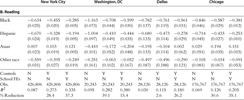
The dependent variable in each column is the state assessment in that subject taken during the 2008–09 school year. For New York City, these are the New York State mathematics and English Language Arts (ELA) exams. For Washington, DC, these are the District of Columbia Comprehensive Assessment System (DC-CAS) mathematics and reading exams. For Dallas, these are the Texas Assessment of Knowledge and Skills (TAKS) mathematics and reading exams (English versions). For Chicago, these are the Illinois Standards Achievement Test (ISAT) mathematics and reading exams. All test scores are standardized to have mean zero and standard deviation one within each grade. Non-Hispanic whites are the omitted race category, so all of the race coefficients are gaps relative to that group. The New York City and Chicago specifications include students in grades three through eight. Washington, DC, includes students in grades three through eight and ten. Dallas includes students in grades three through five. The first specification for each city estimates the raw racial test score gap in each city and does not include any other controls. The second specification for each city includes controls for gender, free lunch status, English language learner (ELL) status, special education status, age in years (linear, quadratic, and cubic terms), census block group income quintile dummies, and missing dummies for all variables with missing data. The third specification includes the same set of controls as well as school fixed effects. Age, special education status, and income data are not available in the Chicago data. Standard errors, located in parentheses, are clustered at the school level. Percent reduction refers to the percent by which the magnitude of the coefficient on black is reduced relative to the coefficient on black in the preceding column. See data appendix for details regarding sample and variable construction.
In NYC, blacks trail whites by 0.696 (0.024) standard deviations, Hispanics trail whites by 0.615 (0.023), and Asians outpace whites by 0.266 (0.022) in the raw data. Adding sex, free lunch status, ELL status, special education status, age (including quadratic and cubic terms), and income quintiles reduces these gaps to 0.536 (0.020) for blacks and 0.335 (0.018) for Hispanics. Asians continue to outperform other racial groups. Including school fixed effects further suppresses racial differences for blacks and Hispanics—yielding gaps of 0.346 (0.005) and 0.197 (0.005), respectively. The Asian gap increases modestly with the inclusion of school fixed effects.
Dallas follows a pattern similar to NYC—there is a black-white gap of 0.690 (0.124) in the raw data which decreases to 0.678 (0.108) with the inclusion of controls, and 0.528 (0.031) with school fixed effects. Asians and Hispanics in Dallas follow a similar pattern to that documented in NYC. Both Chicago and Washington, DC, have raw racial gaps that hover around one standard deviation for blacks and 0.75 for Hispanics. Accounting for differences in school assignment reduces the black-white gaps to 0.657 (0.029) in DC and 0.522 (0.011) in Chicago—roughly half of the original gaps. Asians continue to outpace all racial groups in Chicago and are on par with whites in Washington, DC.
Panel B of Table 13 estimates racial differences in reading achievement across our four cities. Similar to the results presented earlier using nationally representative samples, racial gaps on reading assessments are smaller than those on math assessments. In NYC, the raw gap is 0.634 (0.025) and the gap is 0.285 (0.005) with controls and school fixed effects. Dallas contains gaps of similar magnitude to those in NYC and adding school fixed effects has little effect on racial disparities. Chicago and Washington, DC, trail the other cities in the raw gaps—0.846 (0.046) and 1.163 (0.073) respectively—but these differences are drastically reduced after accounting for the fact that blacks and whites attend different schools. The Chicago gap, with school fixed effects, is 0.381 (0.012) (45% of the original gap) and the corresponding gap in DC is 0.599 (0.030). These gaps are strikingly similar in magnitude to racial differences in national samples such as ELCS-K and CNLSY79, suggesting that biased sampling is not a first-order problem.
Thus far, we have concentrated on average achievement across grades three through eight in NYC, Chicago, and DC, and grades three through five in Dallas. Our analysis of ECLS suggests that racial gaps increase over time. Krueger and Whitmore (2001) and Phillips et al. (1998b) also find that the black-white achievement gap widens as children get older, which they attribute to the differential quality of schools attended by black and white students. Figure 3 plots the raw black-white achievement gap in math (Panel A) and reading (Panel B) for all grades available in each city. In math, DC shows a remarkable increase in the gap as children age—increasing from 0.990 (0.077) in third grade to 1.424 (0.174) in eighth grade. The gap in NYC also increased with age, but much less dramatically. Racial disparities in Chicago are essentially flat across grade levels, and, if anything, racial differences decrease in Dallas. A similar pattern is observed in reading: the gap in DC is increasing over time whereas the gap in other cites is relatively flat. The racial achievement gap in reading in DC is roughly double that in any other city. Figure 4 provides similar data for Hispanics. Hispanics follow a similar, but less consistent, pattern as blacks.
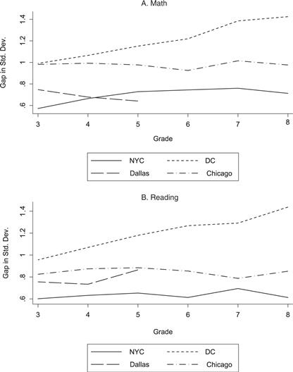
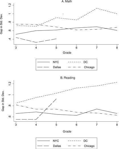
In NYC and Dallas, we were able to obtain data on classroom assignments that allow us to estimate models with teacher fixed effects. In elementary school, we assign the student’s main classroom teacher. In middle schools we assign teachers according to subject: for math (resp. ELA) assessment scores, we compare students with the same math (resp. ELA) teacher. In Dallas, there are 1950 distinct teachers in the sample, with an average of 14 students per teacher. In New York City, there are 16,398 ELA teachers and 16,069 math teachers, with an average of about 25 students per teacher (note that in grades three through five, the vast majority of students have the same teacher for both ELA and math, so the actual number of distinct teachers in the dataset is 20,064.)
Table 14 supplements our analysis by including teacher fixed effects in NYC (Panel A) and Dallas (Panel B) for both math and reading. Each city contains four columns, two for math and two for reading. For comparison, the odd-numbered columns are identical to the school fixed effects specifications in Table 13, but estimated on a sample of students for which we have valid information on their classroom teacher. This restricted sample is 92% of the original for NYC and 99% of the original for Dallas. The even-numbered columns contain teacher fixed effects. Consistent with the analysis in ECLS-K, accounting for sorting into classrooms has a modest marginal effect on the racial achievement gap beyond the inclusion of school fixed effects. The percent reduction in the black coefficient in NYC is 20.0% in math and 25.0% in reading. In Dallas, these reductions are 0.9% and 3.0%, respectively.
Table 14
Racial achievement gap in urban districts: accounting for teachers.
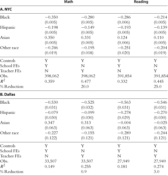
The dependent variable in each column is the state assessment in that subject taken during the 2008–09 school year. For New York City, these are the New York State mathematics and English Language Arts (ELA) exams. For Dallas, these are the Texas Assessment of Knowledge and Skills (TAKS) mathematics and reading exams (English versions). All test scores are standardized to have mean zero and standard deviation one within each grade. Non-Hispanic whites are the omitted race category, so all of the race coefficients are gaps relative to that group. The New York City specifications include students in grades three through eight. The Dallas specifications include students in grades three through five. All specifications include controls for gender, free lunch status, English language learner (ELL) status, special education status, age in years (linear, quadratic, and cubic terms), census block group income quintile dummies, and missing dummies for all variables with missing data. Odd-numbered columns include school fixed effects, whereas even-numbered columns include teacher fixed effects. The samples are restricted to students for whom teacher data in the relevant subject are available. Standard errors are located in parentheses. Percent reduction refers to the percent by which the magnitude of the coefficient on black is reduced relative to the coefficient on black in the preceding column. See data appendix for details regarding sample and variable construction.
Table 15 concludes our analysis of our school district administrative files by investigating the source of the racial achievement gap in NYC across particular skills tested. The math section of the NYC state assessment is divided into five strands: number sense and operations, algebra, geometry, measurement, and statistics and probability. ELA exams are divided into three standards for grades three through eight: (1) information and understanding; (2) literary response and expression; and (3) critical analysis and evaluation. The information and understanding questions measure a student’s ability to gather information from spoken language and written text and to transmit knowledge orally and textually. Literary response and expression refers to a student’s ability to make connections to a diverse set of texts and to speak and write for creative expression. Critical analysis and evaluation measures how well a student can examine an idea or argument and create a coherent opinion in response. There is no clear pattern in the emphasizing or deemphasizing of particular topics between third and eighth grades. The ELA exams focus more heavily on information and understanding and literary response and expression than on critical analysis and evaluation across all years tested. The math exams focus heavily on number sense until eighth grade, when the focus shifts to algebra and geometry. There are also segments of geometry in fifth grade and statistics and probability in seventh grade.
Table 15
Unadjusted means on questions assessing specific sets of skills, NYC.
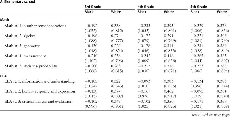
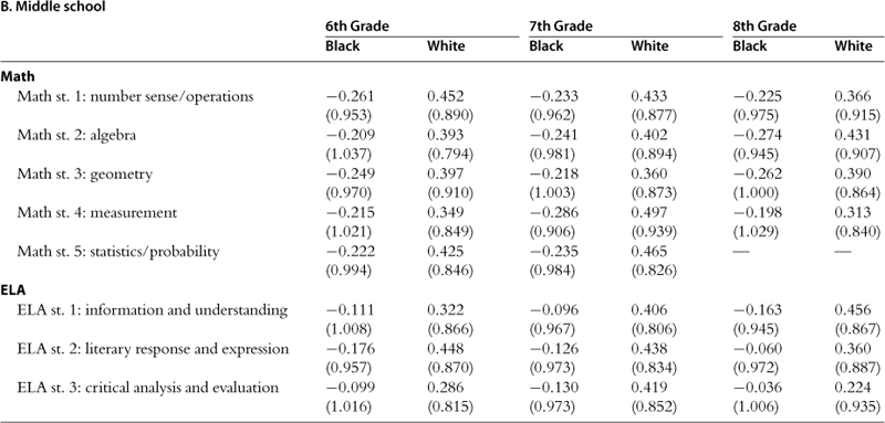
Entries are unadjusted mean percentage of items correct on specific areas of questions on the New York State assessments in mathematics and English Language Arts (ELA) in third through eighth grades in New York City, which are then standardized across the entire sample of test takers for each grade, so that units are standard deviations relative to the mean. Dashes indicate that Statistics/Probability was not included in the eighth grade mathematics exam. Standard deviations are located in parentheses.
The most striking observation about Table 15 is how remarkably robust the racial achievement gap in NYC is across grade levels and sets of skills tested. There are substantial racial gaps on every skill at every grade level. The disparities in reading achievement are roughly halfas large as the disparities in math.
Putting the pieces together, there are four insights gleaned from our analysis in this section. First, racial achievement gaps using district administrative files, which contain all students in a school district, are similar in magnitude to those estimated using national samples. Second, the evidence as to whether gaps increase over time is mixed. Washington, DC, provides the clearest evidence that black and white paths diverge in school. Patterns from other cities are less clear. Third, school fixed effects explain roughly fifty percent of the gap; adding teacher fixed effects explains about twenty-three percent more in NYC and only about two percent more in Dallas. Fourth, and perhaps most troubling, black students are behind on every aspect of the achievement tests at every grade.
6 The racial achievement gap in high school
We conclude our descriptive analysis of the racial achievement gap with high school-aged students using the National Education Longitudinal Survey (NELS).46 The NELS consists of a nationally representative group of students who were in eighth grade in 1988 when the baseline survey and achievement test data were collected. Students were resurveyed in 1990 at the end of their tenth grade year and again in 1992 at the anticipated end of their high school career. All three waves consist of data from a student questionnaire, achievement tests, a school principal questionnaire, and teacher questionnaires; 1990 and 1992 follow-ups also include a dropout questionnaire, the baseline and 1992 follow-up also surveyed parents, and the 1992 follow-up contains student transcript information. NELS contains 24,599 students, in 2963 schools and 5351 math, science, English, and history classrooms initially surveyed in the baseline year. Eighty-two percent of these students completed a survey in each of the first three rounds.
The primary outcomes in the NELS data are four exams: math, reading comprehension, science, and social studies (history/citizenship/government). In the base year (eighth grade), all students took the same set of tests, but in order to avoid problematic “ceiling” and “floor” effects in the follow-up testing (tenth and twelfth grades for most participants) students were given test forms tailored to their performance in the previous test administration. There were two reading test forms and three math test forms; science and social studies tests remained the same for all students. Test scores were determined using Item Response Theory (IRT) scoring, which allowed the difficulty of the test taken by each student to be taken into account in order to estimate the score a student would have achieved for any arbitrary set of test items. Table A.12 provides descriptive statistics.
Table 16 provides estimates of the racial achievement gap in high school across four subjects. For each grade, we estimate four empirical models. We begin with raw racial differences, which are displayed in the first column under each grade. Then, we add controls for race, gender, age (linear, quadratic, and cubic terms), family income, and dummies for parents’ levels of education. The third empirical model includes school fixed effects and the fourth includes teacher fixed effects. The raw black-white gap in eighth grade math is 0.754 (0.025) standard deviations. Adding controls reduces the gap to 0.526 (0.021), and adding school fixed effects reduces the gap further to 0.400 (0.021), which is similar to the eighth grade disparities reported in ECLS. Including teacher fixed effects reduces the gap to 0.343 (0.031) standard deviations. In 10th and 12th grade, black-white disparities range from 0.734 (0.038) in the raw data to 0.288 (0.060) with teacher fixed effects in 10th grade, and 0.778 (0.045) to 0.581 (0.089) in 12th grade. Hispanics follow a similar trend, but the achievement gaps are nearly 40% smaller. In the raw data, Asians are the highest-performing ethnic group in eighth through twelfth grades. Including teacher fixed effects, however, complicates the story. Asians are 0.127 standard deviations ahead of whites in eighth grade. This gap diminishes over time and, by twelfth grade, Asian students trail whites when they have the same teachers.
Table 16
Evolution of the achievement gap overtime, NELS.
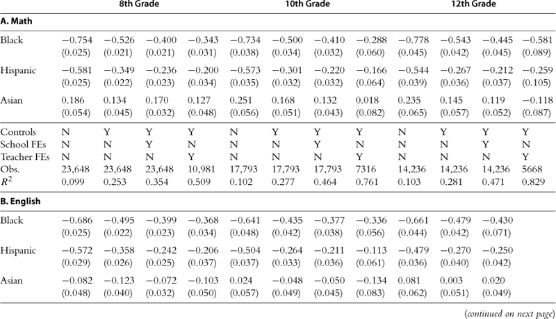
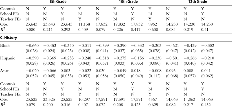
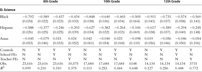
The dependent variable in each column is the NELS test score in the designated subject and grade. Test scores are IRT scores, normalized to have mean zero and standard deviation one in each grade. Non-Hispanic whites are the omitted race category, so all of the race coefficients are gaps relative to that group. The first specification for each grade and subject estimates the raw racial test score gap in that grade and only include race dummies and a dummy for missing race. The second specification for each grade and subject includes controls for gender, age (linear, quadratic, and cubic terms), family income, and dummies that indicate parents’ level of education, as well as missing dummies for all variables with missing data. The third specification includes the same set of controls as well as school fixed effects. For grades eight through twelve of math and science, and for grades eight and ten of English and history, the fourth specification includes the same set of controls as well as teacher fixed effects. For grade twelve of English and history, teacher data were not collected in the second follow-up year of the NELS, so teacher fixed effects cannot be included. Standard errors, located in parentheses, are clustered at the school level.
Panels B, C, and D of Table 16, which estimate racial achievement gaps in English, history, and science, respectively, all show magnitudes and trends similar to those documented above in math. Averaging across subjects, the black-white gap in eighth grade is roughly 0.7 standard deviations. An identical calculation for Hispanics yields a gap of just under 0.6 standard deviations. Asians are ahead in math and on par with whites in all other subjects. In twelfth grade, black students significantly trail whites in science and math (0.911 (0.041) and 0.778 (0.045) standard deviations, respectively) and slightly less so in history and English. Hispanics and Asians demonstrate patterns in twelfth grade that are very similar to their patterns in eighth grade.
To close our analytic pipeline from nine months old to high school graduation, we investigate racial differences in high school graduation or GED acquisition within five years of their freshman year in high school [not shown in tabular form]. In the raw data, blacks are twice as likely as whites to not graduate from high school or receive a GED within five years of entering high school. Accounting for math and reading achievement scores in eighth grade explains all of the racial gap in graduation rates. Hispanics are 2.2 times more likely not to graduate and these differences are reduced to thirty percent more likely after including eighth grade achievement.
We learn four points from NELS. First, achievement gaps continue their slow divergence in the high school years. Second, gaps are as large in science and history as they are in subjects that are tested more often, such as math and reading. Third, similarly as in the preceding analysis, a substantial racial achievement gap exists after accounting for teacher fixed effects. Fourth, the well-documented disparities in graduation rates can be explained by eighth grade test scores. The last result is particularly striking.
7 Interventions to foster human capital in school-aged
CHILDREN
In an effort to increase achievement and narrow differences between racial groups, school districts have become laboratories of innovative reforms, including smaller schools and classrooms (Nye, 1995; Krueger, 1999), mandatory summer school (Jacob and Lefgren, 2004), merit pay for principals, teachers, and students (Podgursky and Springer, 2007; Fryer, 2010), after-school programs (Lauer et al., 2006), budget, curricula, and assessment reorganization (Borman et al., 2007), policies to lower the barrier to teaching via alternative paths to accreditation (Decker et al., 2004; Kane et al., 2008), single-sex education (Shapka and Keating, 2003), data-driven instruction (Datnow et al., 2008), ending social promotion (Greene and Winters, 2006), mayoral/state control of schools (Wong and Shen, 2002, 2005; Henig and Rich, 2004), instructional coaching (Knight, 2009), local school councils (Easton et al., 1993), reallocating per-pupil spending (Mar-low, 2000; Guryan, 2001), providing more culturally sensitive curricula (Protheroe and Barsdate, 1991; Thernstrom, 1992; Banks, 2001, 2006), renovated and more technologically savvy classrooms (Rouse and Krueger, 2004; Goolsbee and Guryan, 2006), professional development for teachers and other key staff (Boyd et al., 2008; Rockoff, 2008), and getting parents to be more involved (Domina, 2005).
The evidence on the efficacy of these investments is mixed. Despite their intuitive appeal, school choice, summer remediation programs, and certain mentoring programs show no effect on achievement (Krueger and Zhu, 2002; Walker and Vilella-Velez, 1992; Bernstein et al., 2009). Financial incentives for students, smaller class sizes, and bonuses for teachers in hard-to-staff schools show small to modest gains that pass a cost-benefit analysis (Fryer, 2010; Schanzenbach, 2007; Jacob and Ludwig, 2008). It is imperative to note: these programs have not been able to substantially reduce the achievement gap even in the most reform-minded school systems.
Even more aggressive strategies that place disadvantaged students in better schools through busing (Angrist and Lang, 2004) or significantly alter the neighborhoods in which they live (Jacob, 2004; Kling et al., 2007; Sanbonmatsu et al., 2006; Turney et al., 2006) have left the racial achievement gap essentially unchanged.
Table 17 describes seventeen additional interventions designed to increase achievement in public schools.47 The first column lists the program name, the second column reports the grades treated, and the third column provides a brief description of each intervention. The final two columns provide information on the magnitude of the reported effect and a reference. The bulk of the evidence finds little to no effect of these interventions. Three programs seem to break this mold: Mastery Learning, Success for All, and self-affirmation essay writing. Mastery learning is a group-based, teacher-paced instructional model that is based on the idea that students must attain a level of mastery on a particular objective before moving on to a new objective. Guskey and Gates (1985) perform a meta-analysis of thirty-five studies on this instructional strategy and find that the average achievement effect size from mastery learning programs was 0.78 standard deviations. The effect sizes from within individual studies, however, ranged from 0.02 to 1.70 and varied significantly depending on the age of the students and the subject tested (Guskey and Gates, 1985).
Table 17
School-age interventions to increase achievement.
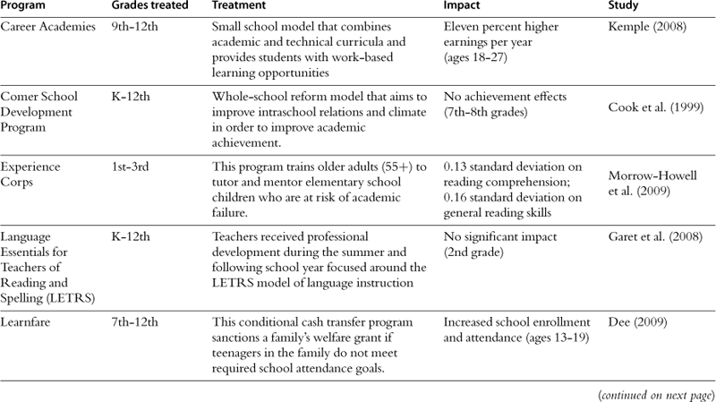

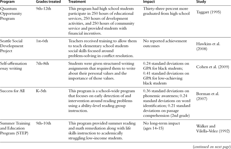
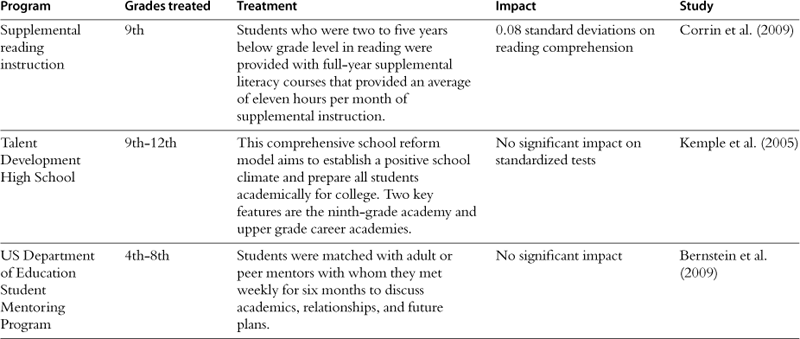
The set of interventions included in this table were generated using a two-step search process. First, a keyword search for for “school-aged interventions” was performed in Google Scholar, JSTOR, and the National Bureau of Economic Research database. Second, we examined all of the available reports for the appropriate age groups from the What Works Clearinghouse of IES. From the original list, we narrowed our focus to those programs that contained credible identification and were large enough in scale to possibly impact achievement gaps overall.
Success for All is a school-level elementary school intervention that focuses on improving literacy outcomes for all students in order to improve overall student achievement that is currently used in 1200 schools across the country (Borman et al., 2007). The program is designed to identify and address deficiencies in reading skills at a young age using a variety of instruction strategies, ranging from cooperative learning to data-driven instruction. Borman et al. (2007) use a cluster randomized trial design to evaluate the impacts of the Success for All model on student achievement. Forty-one schools from eleven states volunteered and were randomly assigned to either the treatment or control groups. Borman et al. (2007) find that Success for All increased student achievement by 0.36 standard deviations on phonemic awareness, 0.24 standard deviations on word identification, and 0.21 standard deviations on passage comprehension.
The self-affirmation essay writing intervention was intended specifically to improve the academic achievement of minorities by reducing the impact of stereotype threat. Seventh grade students were randomly assigned to either a treatment or control group. Both groups were given structured writing assignments three to five times over the course of two school years, but the treatment group was instructed to write about their personal values and why they were important, while the control group was given neutral essay topics. Cohen et al. (2009) find that for black students, this intervention increased GPA by 0.24 points and that the impact was even greater for low-achieving black students (0.41 GPA points). They also find that the program reduced the probability of being placed in remedial classes or being retained in a grade for low-achieving black students. It is unclear what the general equilibrium effects of such psychological interventions are.
Despite trillions spent, there is not one urban school district that has ever closed the racial achievement gap. Figures 5 and 6 show the achievement gap in percentage of students proficient for their grade level across eleven major US cities who participate in the National Assessment of Educational Progress (NAEP)—a nationally representative set of assessments administered every two years to fourth, eighth, and twelfth graders that covers various subject areas, including mathematics and reading.48
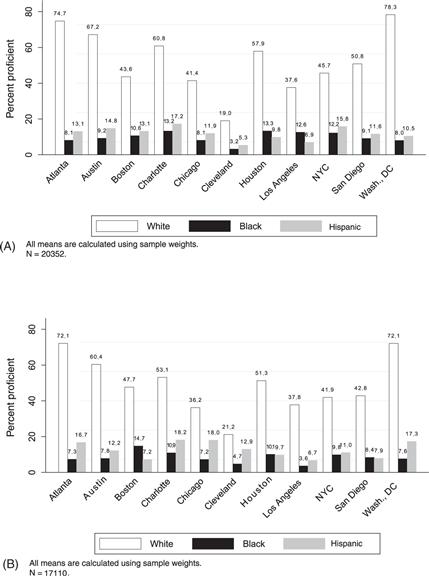
Figure 5 (A) NAEP 2007 proficiency levels by city and race: 4th grade reading. (B) NAEP 2007 proficiency levels by city and race: 8th grade reading.
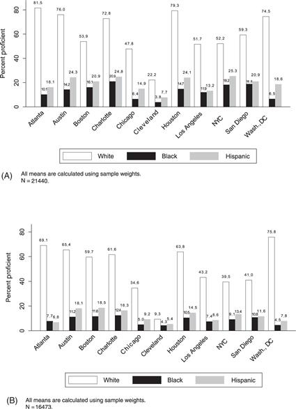
Figure 6 (A) NAEP2007 proficiency levels by city and race: 4th grade math. (B) NAEP2007 proficiency levels by city and race: 8th grade math.
In every city there are large racial differences. In the Trial Urban District Assessment, among fourth graders, 43.2% of whites, 12% of blacks, and 16% of Hispanics are proficient in reading. In math, these numbers are 50.9, 14, and 20.9, respectively. Similarly, among eighth graders, 40.4% of whites, 10.6% of blacks, and 13.2% of Hispanics score proficient in reading. Math scores exhibit similarly marked racial differences. Washington, DC, has the largest achievement gap of participating cities in NAEP; there is a roughly seventy percent difference between blacks and whites on both subjects and both grade levels. At the other end of the spectrum, Cleveland has the smallest achievement gap—less than seventeen percentage points separate racial groups. Unfortunately, Cleveland’s success in closing the achievement gap is mainly due to the dismal performance of whites in the school district and not due to increased performance of black students. Remarkably, there is very little variance in the achievement of minority students across NAEP districts. There is not one school district in NAEP in which more than twenty-one percent of black students are proficient in reading or math.
The lack of progress has fed into a long-standing and rancorous debate among scholars, policymakers, and practitioners as to whether schools alone can close the achievement gap, or whether the issues children bring to school as a result of being reared in poverty are too much for even the best educators to overcome. Proponents of the school-centered approach refer to anecdotes of excellence in particular schools or examples of other countries where poor children in superior schools outperform average Americans (Chenoweth, 2007). Advocates of the community-focused approach argue that teachers and school administrators are dealing with issues that actually originate outside the classroom, citing research that shows racial and socioeconomic achievement gaps are formed before children ever enter school (Fryer and Levitt, 2004, 2006) and that one-third to one-half of the gap can be explained by family-environment indicators (Phillips et al., 1998a,b; Fryer and Levitt, 2004).49 In this scenario, combating poverty and related social ills directly and having more constructive out-of-school time may lead to better and more focused instruction in school. Indeed, Coleman et al. (1966), in their famous report on equality of educational opportunity, argue that schools alone cannot solve the problem of chronic underachievement in urban schools.
The Harlem Children’s Zone (HCZ)—a 97-block area in central Harlem, New York, that combines reform-minded charter schools with a web of community services designed to ensure the social environment outside of school is positive and supportive for children from birth to college graduation—provides an extremely rare opportunity to understand whether communities, schools, or a combination of the two are the main drivers of student achievement.
Dobbie and Fryer (2009) use two separate statistical strategies to estimate the causal impact of attending the charter schools in the HCZ. First, they exploit the fact that HCZ charter schools are required to select students by lottery when the number of applicants exceeds the number of available slots for admission. In this scenario, the treatment group is composed of students who are lottery winners and the control group consists of students who are lottery losers. The second identification strategy explored in Dobbie and Fryer (2009) uses the interaction between a student’s home address and her cohort year as an instrumental variable. This approach takes advantage of two important features of the HCZ charter schools: (1) anyone is eligible to enroll in HCZ’s schools, but only students living inside the Zone are actively recruited by HCZ staff; and (2) there are cohorts of children that are ineligible due to the timing of the schools’ opening and their age. Both statistical approaches lead to the same result: HCZ charter schools are effective at increasing the achievement of the poorest minority children.
Figure 7A and B provide a visual representation of the basic results from Dobbie and Fryer (2009). Figure 7A plots yearly, raw, mean state math test scores, from fourth to eighth grade, for four subgroups: lottery winners, lottery losers, white students in New York City public schools and black students in New York City public schools. Lottery winners are comprised of students who either won the lottery or who had a sibling who was already enrolled in the HCZ Promise Academy. Lottery losers are individuals who lost the lottery and did not have a sibling already enrolled. These represent reduced form estimates.
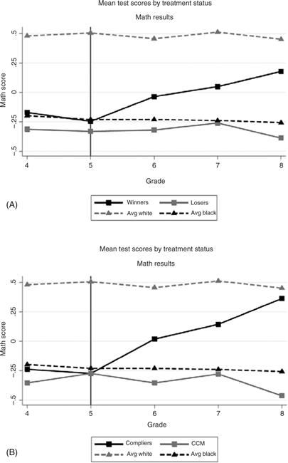
Figure 7 Student achievement in HCZ-math. (A) Reduced Form result. (B) TOT results. Notes: Lottery winners are students who receive a winning lottery number or who are in the top ten of the waitlist. Test scores are standardized by grade to have mean zero and standard deviation one in the entire New York City sample. The CCM is the estimated test score for those in the control group who would have complied if they had received a winning lottery number.
In fourth and fifth grade, before they enter the middle school, math test scores for lottery winners, losers, and the typical black student in New York City are virtually identical, and roughly 0.75 standard deviations behind the typical white student.50 Lottery winners have a modest increase in sixth grade, followed by a more substantial increase in seventh grade and even larger gains by their eighth-grade year.
The “Treatment-on-Treated” (TOT) estimate, which is the effect of actually attending the HCZ charter school, is depicted in Panel B of Fig. 7. The TOT results follow a similar pattern, showing remarkable convergence between children in the middle school and the average white student in New York City. After three years of “treatment,” HCZ Promise Academy students have nearly closed the achievement gap in math—they are behind their white counterparts by 0.121 standard deviations (p-value = 0.113). If one adjusts for gender and free lunch, the typical eighth grader enrolled in the HCZ middle school outscores the typical white eighth grader in New York City public schools by 0.087 standard deviations, though the difference is not statistically significant (p-value = 0.238).
Figure 8A plots yearly state ELA test scores, from fourth to eighth grade. Treatment and control designations are identical to those in Fig. 7A. In fourth and fifth grades, before they enter the middle school, ELA scores for lottery winners, losers, and the typical black student in NYC are not statistically different, and are roughly 0.65 standard deviations behind the typical white student.51 Lottery winners and losers have very similar ELA scores from fourth through seventh grade. In eighth grade, HCZ charter students distance themselves from the control group. These results are statistically meaningful, but much less so than the math results. The TOT estimate, depicted in Panel B of Fig. 8, follows an identical pattern with marginally larger differences between enrolled middle-school students and the control group. Adjusting for gender and free lunch pushes the results in the expected direction.52
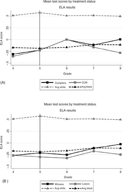
Figure 8 Student achievement in HCZ-ELA. (A) Reduced Form Results. (B) TOT Results. Notes: Lottery winners are students who receive a winning lottery number or who are in the top ten of the waitlist. Test scores are standardized by grade to have mean zero and standard deviation one in the entire New York City sample. The CCM is the estimated test score for those in the control group who would have complied if they had received a winning lottery number.
7.1 What do the results from HCZ tell us about interventions to close the achievement gap?
There are six pieces of evidence that, taken together, suggest schools alone can dramatically increase the achievement of the poorest minority students—other community and broader investments may not be necessary. First, Dobbie and Fryer (2009) find no correlation between participation in community programs and academic achievement. Second, the IV strategy described above compares children inside the Zone’s boundaries relative to other children in the Zone who were ineligible for the lottery, so the estimates are purged of the community bundle. Recall that IV estimates are larger than the lottery estimates, however, suggesting that communities alone are not the answer. Third, Dobbie and Fryer (2009) report that children inside the Zone garnered the same benefit from the schools as those outside the Zone, suggesting that proximity to the community programs is unimportant. Fourth, siblings of HCZ students who are in regular public schools, but likely have better-than-average access and information about HCZ community programs, have marginally lower absence rates but their achievement is unchanged (Dobbie and Fryer, 2009).
The final two pieces of evidence are taken from interventions outside of HCZ. The Moving to Opportunity experiment, which relocated individuals from high-poverty to low-poverty neighborhoods while keeping the quality of schools roughly constant, showed small positive results for girls and negative results for boys (Sanbonmatsu et al., 2006; Kling et al., 2007). This suggests that a better community, as measured by poverty rate, does not significantly raise test scores if school quality remains essentially unchanged.
The last pieces of evidence stem from the rise of a new literature on the impact of charter schools on achievement. While the bulk of the evidence finds only modest success (Hanushek et al., 2005; Hoxby and Rockoff, 2004; Hoxby and Murarka, 2009), there are growing examples of success that is similar to that achieved in HCZ—without community or broader investments. The Knowledge is Power Program (KIPP) is the nation’s largest network of charter schools. Anecdotally, they perform at least as well as students from HCZ on New York state assessments.53 Angrist et al. (2010) perform the first quasi-experimental analysis of a KIPP school, finding large impacts on achievement. The magnitude of the gains are strikingly similar to those in HCZ. Figure 9 plots the reduced form effect of attending KIPP in Lynn, Massachusetts. Similar to the results of KIPP, Abdulkadiroglu et al. (2009) find that students enrolled in oversubscribed Boston charter schools with organized lottery files gain about 0.17 standard deviations per year in ELA and 0.53 standard deviations per year in math.54
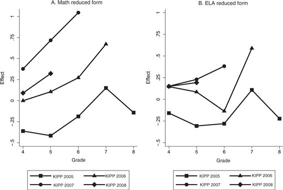
Figure 9 Student achievement in KIPP Lynn.55
8 Conclusion
In 1908, W.E.B Dubois famously noted that “the problem of the 20th century is the problem of the color line.” America has undergone drastic changes in 102 years. The problem of the 21st century is the problem of the skill gap. As this chapter attempts to make clear, eliminating the racial skill gap will likely have important impacts on income inequality, unemployment, incarceration, health, and other important social and economic indices. The problem, to date, is that we do not know how to close the achievement gap.
Yet, there is room for considerable optimism. A key difference between what we know now and what we knew even two years ago lies in a series of ”existence proofs” in which poor black and Hispanic students score on par with more affluent white students. That is, we now know that with some combination of investments, high achievement is possible for all students. That is an important step forward. Ofcourse, there are many questions as to how one can use these examples to direct interventions that have the potential to close the achievement gap writ large.56 An economist’s solution might be to create a market for gap-closing schools with high-powered incentives for entrepreneurs to enter. The government’s role would not be to facilitate the daily workings of the schools; it would simply fund those schools that close the achievement gap and withhold funds from those that do not. The non-gap-closing schools would go out of business and would be replaced by others that are more capable. In a rough sense, this is what is happening in Louisiana post-Hurricane Katrina, what cities such as Boston claim to do, and what reform-minded school leaders such as Chancellor Joel Klein in New York City have been trying accomplish within the constraints of the public system.
A second, potentially more politically expedient, way forward is to try and understand what makes some schools productive and others not. Hoxby and Murarka (2009) and Abdulkadiroglu et al. (2009) show that there is substantial variance in the treatment effect of charter schools—even though all are free from most constraints of the public system and the vast majority do not have staffs under collective bargaining agreements. Investigating this variance and its causes could reveal important clues about measures that could be taken to close the racial achievement gap.
Independent of how we get there, closing the racial achievement gap is the most important civil rights battle of the twenty-first century.
Appendix Data description
A.1 National longitudinal survey of youth 1979(NLSY79)
The National Longitudinal Survey of Youth, 1979 Cohort (NLSY79) is a panel data set with data from 12,686 individuals born between 1957 and 1964 who were first surveyed in 1979 when they were between the ages of 14 and 22. The survey consists of a nationally representative cross-section sample as well as a supplemental over-sample of blacks, Hispanics, and low-income whites. In our analysis, we include only the nationally representative cross-section and the over-samples of blacks and Hispanics. We drop 2923 people from the military and low-income white oversamples and 4 more who have invalid birth years (before 1957 or after 1964). The 5386 individuals who were born before 1962 are also not included in our analysis.
AFQT score
The Armed Forces Qualification Test (AFQT) is a subset of four tests given as part of the Armed Services Vocational Aptitude Battery (ASVAB). AFQT scores as reported in the 1981 survey year are used. Scores for an individual were considered missing if problems were reported, if the procedures for the test were altered, or if no scores are reported (either valid or invalid skip) on the relevant ASVAB subtests.
The AFQT score is the sum of the arithmetic reasoning score, the mathematics knowledge score, and two times the verbal composite score. This composite score is then standardized by year of birth (in order to account for natural score differences arising because of differences in age when the test was taken) and then across the whole sample, excluding those with missing AFQT scores.
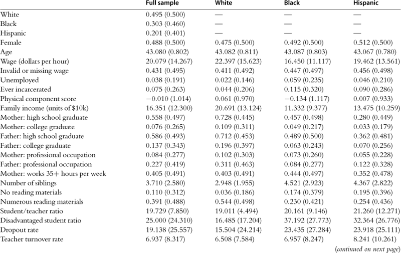
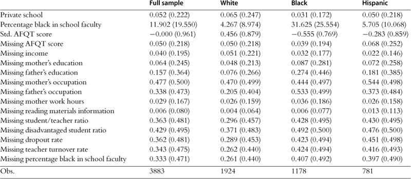
The variable AFQT2 is simply constructed by squaring the standardized AFQT score.
Age
In order to determine an individual’s age, we use the person’s year of birth. The birth year given in 1981 (the year participants took the AFQT) is used if available; otherwise the year of birth given at the beginning of the data collection in 1979 is used. Those who report birth years earlier than 1957 or later than 1964 are dropped from our sample, as these birth years do not fit into the reported age range of the survey.
Additionally, those who were born after 1961 were excluded from analyses. Those born in 1961 or earlier were at least 18 at the time of taking the AFQT and therefore were more likely to have already entered the labor force, which introduces the potential for bias in using AFQT to measure achievement. See Neal and Johnson (1996) for a full explanation.
Ever incarcerated
In order to construct this variable, we use the fact that the residence of a respondent is recorded each time they are surveyed. One of the categories for type of residence is “jail”. Therefore, the variable “ever incarcerated” is equal to one if for any year of the survey the individual’s type of residence was “jail”. We also include in our measure those who were not incarcerated at any point during the survey but who had been sentenced to a corrective facility before the initial 1979 survey.
Family income
To construct family income, we use the total net family income variables from 1979, 1980, and 1981. We convert all incomes into 1979 dollars, and then use the most recent income available.
Numerous reading materials
We classify a person as having “numerous reading materials” if they had magazines, newspapers, and a library card present in their home environment at age 14.
Parent occupation
To construct the dummies for having a mother (father) with a professional occupation, we use the variable which gives the occupational code of the adult female (male) present in the household at age 14. We classify mothers (fathers) as professionals if they have occupational codes between 1 and 245. This corresponds to the following two occupational categories: professional, technical, and kindred; and managers, officials, and proprietors.
Physical health component score
This variable is constructed within the data set using the questions asked by the SF-12 portion of the 2006 administration of the surveys. For the analysis, the physical component score (PCS) is standardized across all individuals for whom a score is available. Those without a valid PCS are not included in the analysis.
Race
A person’s race is coded using a set of mutually exclusive dummy variables from the racial/ethnic cohort of the individual from the screener. Individuals are given a value of one in one of the three dummy variables—white, black, or Hispanic. All respondents have a value for this race measure.
Sex
A person’s sex was coded as a dummy variable equal to one if the person is male and zero if the person is female. Preference was given for the reported sex in 1982; if this was unavailable, the sex reported in 1979 was used.
Unemployed
The variable “unemployed” is a binary variable that is equal to one if the person’s employment status states that they are unemployed. Those whose employment status states that they are not in the labor force are excluded from labor force participation analyses.
Wage
Job and wage information are given for up to five jobs per person in 2006, which was the latest year for which published survey results were available. The data contains the hourly compensation and the number of hours worked for each of these jobs, as well as an indicator variable to determine whether each particular job is a current job. The hourly wage from all current jobs is weighted by the number of hours worked at that job in order to determine an individual’s overall hourly wage.
Neal and Johnson (1996) considered wage reports invalid if they were over $75. We do the same, but adjust this amount for inflation; therefore, wages over $115 (the 2006 equivalent of $75 in 1990) are considered to be invalid. Wage is also considered to be missing/invalid if the individual does not have a valid job class for any of the five possible jobs. Individuals with invalid or missing wages are not included in the wage regressions, which use the log of the wage measure as the dependent variable.
A.2 National longitudinal survey of youth 1997 (NLSY97)
The National Longitudinal Survey of Youth, 1997 Cohort (NLSY97) is a panel data set with data from approximately 9000 individuals born between 1980 and 1984 who were first surveyed in 1997 when they were between the ages of 13 and 17.
AFQT score
The Armed Forces Qualification Test (AFQT) is a subset of four tests given as part of the Armed Services Vocational Aptitude Battery (ASVAB). In the NLSY97 data set, an ASVAB math-verbal percent score was constructed. The NLS staff states that the formula they used to construct this score is similar to the AFQT score created by the Department of Defense for the NLSY79, but that it is not the official AFQT score.
The AFQT percentile score created by the NLS was standardized by student age within three-month birth cohorts. We then standardized the scores across the entire sample of valid test scores.
The variable AFQT2 is simply constructed by squaring the standardized AFQT score.
Age
Because wage information was collected in either 2006 or 2007 (discussed below), the age variable needed to be from the year in which the wage data was collected. The age variable was constructed first as two separate age variables—the person’s age in 2006 and the person’s age in 2007—using the person’s birth year as reported in the baseline (1997) survey. The two age variables are then combined, with the age assigned to be the one from the year in which the wage was collected.
All age cohorts were included in the labor force analyses. Because participants were younger during the baseline year of the survey when the AFQT data were collected—all were under the age of 18—they were unlikely to have entered the labor force yet.
Ever incarcerated
In the NLSY97, during each yearly administration of the survey, individuals are asked what their sentence was for any arrests (up to 9 arrests are asked about). Individuals who reported that they were sentenced to “jail”, an “adult corrections institution”, or a “juvenile corrections institution” for any arrest in any of the surveys were given a value of one for this variable; otherwise this variable was coded as zero.
Race
A person’s race is coded using a set of mutually exclusive dummy variables from the racial/ethnic cohort of the individual from the screener. Individuals are given a value of one in one of the four dummy variables—white, black, Hispanic, or mixed race. All respondents have a value for this race measure.
Sex
A person’s sex was coded as a dummy variable equal to one if the person is male and zero if the person is female.
Unemployed
The variable “unemployed” is a binary variable that is equal to one if the person’s employment status states that they are unemployed. Those whose employment status states that they are not in the labor force are excluded from labor force participation analyses.
Wage
Jobs and wage information is given for up to 9 jobs in 2007 and up to 8 jobs in 2007. We are given the hourly compensation and the number of hours worked for each of these jobs, as well as a variable to determine whether each particular job is a current job. The hourly wage from all current jobs is weighted by the number of hours worked at that job in order to determine an individual’s overall hourly wage.
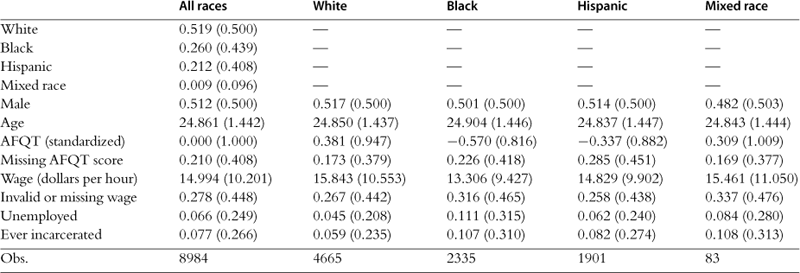
Once again, wages over $115 in 2006 and $119 in 2007 (the equivalent of $75 in 1990) are considered to be invalid. Wage is also considered to be missing/invalid if the individual does not have a valid job class for any of the possible jobs. Individuals with invalid or missing wages are not included in the wage regressions, which use the log of the wage measure as the dependent variable.
Wage in 2007 is converted to 2006 dollars so that the two wage measures are comparable. We use the 2007 wage measure for any individuals for whom it is available; otherwise, we use the 2006 wage measure.
A.3 College & Beyond, 1976 Cohort (C&B)
The College and Beyond Database contains data on 93,660 full-time students who entered thirty-four colleges and universities in the fall of 1951, 1976, or 1989. For this analysis, we focus on the cohort from 1976. The C&B data contain information drawn from students’ applications and transcripts, SAT and ACT scores, as well as information on family demographics and socioeconomic status. The C&B database also includes responses to a survey administered in 1996 to all three cohorts that provides detailed information on post-college labor market outcomes. The response rate to the 1996 survey was approximately 80%.
Income
Income information is reported as fitting into one of a series of income ranges, but these ranges were different in the 1995 and 1996 surveys. For all the possible ranges in each survey year, the individual’s income was assigned to the midpoint of the range (i.e. $40,000 for the $30,000-50,000 range); for less than $10,000, income was assigned to be $5000 (1995 survey). Income less than $1000 income was assigned to be missing because an individual could not have made this sum of money working full-time (1996 survey). For more than $200,000, income was assigned to be $250,000. If available, income reported for 1995 (the 1996 survey) was used; otherwise 1994 annual income (collected in 1995) was used. Individuals with invalid or missing wages are not included in the income regressions, which use the log of the income measure as the dependent variable.
Race
A person’s race is coded using a set of mutually exclusive dummy variables from the racial/ethnic cohort of the individual from the screener. Individuals are given a value of one in one of the five dummy variables—white, black, Hispanic, other race, or missing the race variable.
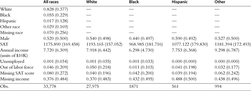
SAT score
The SAT score of an individual is coded as the true value of the combined math and verbal scores, with possible scores ranging between 400 (200 per section) and 1600 (800 per section). Individuals with missing scores are assigned a score of zero and are accounted for using a missing score dummy variable. The square of SAT score was also included in regressions that controlled for educational achievement.
Sex
A person’s sex was coded as a dummy variable equal to one if the person is male and zero if the person is female.
Unemployed
Determining who was unemployed in this data set required a few steps. First, we had to determine who was not working at the time of the survey. This is coded within two variables, one for each survey (1995 and 1996). If an individual reports that they are not working because they are retired or for another reason, we then consider a later question, where they are asked about any times at which they were out of work for 6 months or longer. For those people who stated that they were not currently working, we considered any period of time that included the year of the survey in which they stated they were not working. We then considered the reason they gave for being out of work during that period. If the person stated that they were retired, a student, had family responsibilities, had a chronic illness, or did not need/want to work, we considered them out of the labor force. If a person was not out of the labor force but was not currently working because they were laid off or suitable work was not available, we considered that individual unemployed. Because only 39 people from the entire sample could be considered unemployed, we did not perform analyses using this variable.
A.4 early childhood longitudinal study, birth cohort (ECLS-B)
The Early Childhood Longitudinal Study, Birth Cohort (ECLS-B) is a nationally representative sample of over 10,000 children born in 2001. The first wave of data collection was performed when most of the children were between eight and twelve months of age. The second wave interviewed the same set of children around their second birthday; the third wave was conducted when the children were of preschool age (approximately 4 years old). The data set includes an extensive array of information from parent surveys, interviewer observation or parent-child interactions, and mental and motor proficiency tests. Further details on the study design and data collection methods are available at the ECLS website (http://nces.ed.gov/ecls).
From the total sample, 556 children had no mental ability test score in the first wave. Test scores are missing for an additional 1326 children in the second wave and 1338 children in the third wave. All subjects with missing test scores are dropped from the analysis. This is the only exclusion we make from the sample.57 Throughout the analysis, the results we report are weighted to be nationally representative using sampling weights included in the data set.58
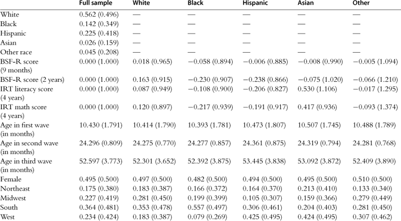
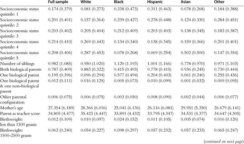
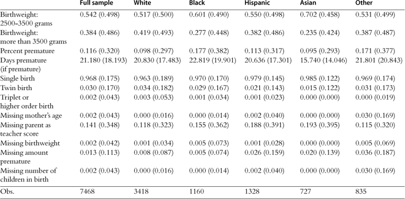
Bayley Short Form—Research Edition (BSF-R)
The BSF-R is an abbreviated version of the Bayley Scale of Infant Development (BSID) that was designed for use in the ECLS to measure the development of children early in life in five broad areas: exploring objects (e.g., reaching for and holding objects), exploring objects with a purpose (e.g., trying to determine what makes the ringing sound in a bell), babbling expressively, early problem solving (e.g., when a toy is out of reach, using another object as a tool to retrieve the toy), and naming objects.59 The test is administered by a trained interviewer and takes twenty-five to thirty-five minutes to complete. A child’s score is reported as a proficiency level, ranging from zero to one on each of the five sections. These five proficiency scores have also been combined into an overall measure of cognitive ability using standard scale units. Because this particular test instrument is newly designed for ECLS-B, there is little direct evidence regarding the correlation between performance on this precise test and outcomes later in life. For a discussion of the validity of this instrument, see Fryer and Levitt (2010, forthcoming). The BSF-R scores have been standardized across the population of children with available scores to have a mean of zero and a standard deviation of one.
Early reading and math scores
As the BSF-R is not developmentally appropriate for preschool-aged children, in order to measure mental proficiency in the third wave (4 years old), a combination of items were used from several assessment instruments. The test battery was developed specifically for use in the ECLS-B and included items from a number of different assessments, including the Peabody Picture Vocabulary Test (PPVT), the Preschool Comprehensive Test of Phonological and Print Processing (Pre-CTOPPP), the PreLAS 2000, and the Test of Early Mathematics Ability-3 (TEMA-3), as well as questions from other studies, including the Family and Child Experiences Study (FACES), the Head Start Impact Study, and the ECLS-K. The assessment battery was designed to test language and literacy skills (including English language skills, emergent literacy, and early reading), mathematics ability, and color knowledge. The cognitive battery was available in both English and Spanish; children who spoke another language were not assessed using the cognitive battery.
The preschool cognitive scores are estimated using Item Response Theory (IRT) modeling based on the set of questions that was administered to each student. The study used IRT modeling to create skill-specific cluster scores that estimate what a student’s performance within a given cluster would have been had the entire set of items been administered. Additionally, scores have been converted to a proficiency probability score that measures a child’s proficiency within a given skill domain and standardized T-scores that measure a child’s ability in comparison to his peers.
Age
Child’s age is coded in three sets of variables, one for each wave of the survey. For the 9-month wave, dummy variables were created for each of the possible one-month age ranges between 8 months and 16 months (inclusive). Children who were younger than 8 months were included in the 8-month variable and children who were older than 16 months were included in the 16-month variable. For the 2-year wave, dummy variables were created for each of the possible one-month age ranges between 23 months and 26 months (inclusive). Children who were younger than 23 months were included in the 23-month variable, while children who were older than 26 months were included in the 26-month variable. For the preschool wave, dummy variables were created for each of the possible one-month age ranges between 47 months and 60 months (inclusive). Children who were younger than 47 months were included in the 47-month variable and children who were older then 60 months were included in the 60-month variable.
Race
Race is defined in a mutually exclusive set of dummy variables, with a child being assigned a value of one for one of white, black, Hispanic, Asian, or other race.
Region
Dummy variables were created for each of four regions of the country: Northeast, Midwest, South, and West.
Sex
The variable for a child’s sex is a binary variable that is equal to one if the child is female and zero if the child is male.
Family structure
This is coded as a set of four dummy variables, each representing a different possible set of parents with whom the child lives: two biological parents, one biological parent, one biological parent and one non-biological parent, and other.
Mother’s age
A continuous variable was created for the age of the child’s mother. Analyses including this variable also included squared, cubic, quartic, and quintic terms. The cubic, quartic, and quintic terms were divided by 100,000 before their inclusion in the regressions.
Number of siblings
Number of siblings is coded as a set of dummy variables, each one representing a different number of siblings. All children with 6 or more siblings are coded in the same dummy variable.
Parent as teacher score
The “parent as teacher” score is coded based on interviewer observations of parent-child interactions in a structured problem-solving environment and is based on the Nursing Child Assessment Teaching Scale (NCATS). The NCATS consists of 73 binary items that are scored by trained observers. The parent component of the NCATS system has 50 items that focus on the parent’s use of a “teaching loop,” which consists of four components: (1) getting the child’s attention and setting up expectations for what is about to be done; (2) giving instructions; (3) letting the child respond to the teaching; and (4) giving feedback on the child’s attempts to complete the task. The parent score ranges from 0 to 50. Analyses including this variable also included squared, cubic, quartic, and quintic terms. The cubic, quartic, and quintic terms were divided by 100,000 before their inclusion in the regressions.
Socioeconomic status
Socioeconomic status is constructed by ECLS and includes parental income, occupation, and education. It is coded as a set of five mutually exclusive and exhaustive dummy variables, each one representing a different socioeconomic status quintile.
Birthweight
The birthweight of the child was coded in a set of four dummy variables: under 1500 grams, 1500–2500 grams, 2500–3500 grams, and over 3500 grams.
Multiple birth indicator
A set of dummy variables were created to indicate how many children were born at the same time as the child: single birth, twin birth, or triplet or higher order birth.
Premature births
Premature births are considered in two different ways. First, a dummy variable is created to classify the child as being born prematurely or not. Then a set of dummy variables were created to capture how early the child was born: less than 7 days, 8–14 days, 15–21 days, etc. in seven day increments up to 77 days premature. Any births more than 77 days premature are coded in the 71 −77 days premature dummy variable.
A.5 collaborative perinatal project (CPP)
The Collaborative Perinatal Project (CPP) consists of over 31,000 women who gave birth in twelve medical centers between 1959 and 1965. All medical centers were in urban areas; six in the Northeast, four in the South, one in the West, and one in the north-central region of the US. Some institutions selected all eligible women, while others took a random sample.60 The socioeconomic and ethnic composition of the participants is representative of the population qualifying for medical care at the participating institutions. These women were re-surveyed when their children were eight months, four years, and seven years old. Follow-up rates were remarkably high: eighty-five percent at eight months, seventy-five percent at four years, and seventy-nine percent at seven years. We only include students in our analysis that had score results for all three tests.61 Our analysis uses data on demographics, measures of home environment, and prenatal factors. In all cases, we use the values collected in the initial survey for these background characteristics.62
Bayley Scales of Infant Development (BSID)
The Bayley Scales of Infant Development (BSID) can be used to measure the motor, language, and cognitive development of infants and toddlers (under three years old). It is therefore used only in the first wave of the CPP. The assessment consists of 45–60 minutes of developmental play tasks administered by a trained interviewer. For use in this analysis, scores were standardized across the entire population. Individuals with scores lower than ten standard deviations below the mean are considered to have missing scores.
Stanford-Binet intelligence scales
The Stanford-Binet Intelligence Scales were used as the main measure of cognitive ability for the second wave of the CPP when the children were four years-old. The scores are standardized across the entire sample of available scores.
Wechsler Intelligence Scale for Children (WISC)
The Wechsler Intelligence Scale for Children (WISC) was used as the main measure of cognitive ability for the third wave of the CPP when the children were seven years-old. The scores are standardized across the entire sample of available scores.
Age
For the first wave of the study (8 months), age is coded as a set of dummy variables representing 5 age ranges: less than 7.5 months, 7.5-8.5 months, 8.5-9 months, 9–10 months, and over 10 months.
In the second (4 years) and third (7 years) waves of the study, age is coded as a continuous variable and given as age of the child in months at the time of the follow-up survey and testing.
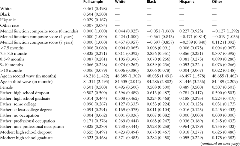
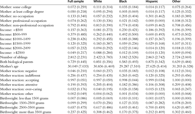
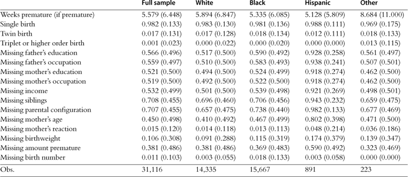
Race
Race is defined in a mutually exclusive set of dummy variables, with a child being assigned a value of one for one of white, black, Hispanic, or other race. Preference is given for the race reported when the child is 8 months; if no race is reported then, race is used as reported at 7 years, then at 3 years, then at 4 years.
Sex
The variable for a child’s sex is a binary variable that is equal to one if the child is female and zero if the child is male. Preference is given for the sex reported when the child is 8 months; if no sex is reported then, sex is used as reported at 7 years, then at 3 years, then at 4 years.
Family structure
A dummy variable is created to indicate whether both the biological mother and biological father are present.
Income
The cumulative income of the family during the first three months of pregnancy is coded as a set of dummy variables representing a range of incomes. Each family is coded within one of the following income ranges: less than $500, $500-1000, $1000-1500, $15002000, $2000-2500, or more than $2500.
Mother’s age
A continuous variable was created for the age of the child’s mother. Analyses including this variable also included squared, cubic, quartic, and quintic terms. The quartic and quintic terms were divided by 1000 before their inclusion in the regressions.
Mother’s reaction to child
A set of dummy variables for the mother’s reaction to the child are included, indicating if the mother is indifferent, accepting, attentive, or over-caring toward the child, or if she behaves in another manner. These dummy variables are constructed by considering the mother’s reaction to and interactions with the child, which are assessed by the interviewer. These dummy variables are not mutually exclusive, as a mother is coded as fitting into each category (negative, indifferent, accepting, attentive, caring, or other) if she fits into that category for any of the measures. Therefore, any mother who falls into different categories for the different measures will be coded with a value of one for multiple dummy variables in this set.
Number of siblings
Number of siblings is coded as a set of dummy variables, each one representing a different number of siblings from zero to six-plus siblings. All children with 6 or more siblings are coded in the same dummy variable.
Parents’ education
A separate set of dummy variables are coded to represent the educational attainment of the child’s mother and father. Each parent’s education is coded as one of : high school dropout (less than 12 years of schooling), high school graduate (12 years of schooling), some college (more than 12 years of schooling but less than 16 years of schooling), or at least college degree (16 or more years of schooling).
Parents’ occupation
A separate set of dummy variables are coded to represent the field of work done by the mother and father of the child. Each parent’s occupational status is coded as one of : no occupation, professional occupation, or non-professional occupation.
Birthweight
The birthweight of the child was given as an amount in pounds and ounces. This measure was first converted to an amount in ounces and the weight in ounces was then converted to a weight in grams. The birthweight of the child was coded in a set of four dummy variables: under 1500 grams, 1500–2500 grams, 2500–3500 grams, and over 3500 grams.
Multiple birth indicator
A set of dummy variables were created to indicate how many children were born at the same time as the child: single birth, twin birth, or triplet or higher order birth.
Prematurity
Premature births are considered in two different ways. First, a dummy variable is created to classify the child as being born prematurely or not. Then a set of dummy variables were created to capture how early the child was born, in weekly increments up to 11 weeks. Any children born more than 11 weeks premature were included in the dummy variable for 11 weeks premature. The amount of time that a child was born prematurely was determined by subtracting the gestation length of the child from 37, which is the earliest gestation period at which a birth is considered full-term.
A.6 early childhood longitudinal study, kindergarten cohort (ECLS-K)
The Early Childhood Longitudinal Study kindergarten cohort (ECLS-K) is a nationally representative sample of 21,260 children entering kindergarten in 1998. Thus far, information on these children has been gathered at seven separate points in time. The full sample was interviewed in the fall and spring of first grade. All of our regressions and summary statistics are weighted, unless otherwise noted, and we include dummy variables for missing data. We describe below how we combined and recoded some of the ECLS variables used in our analysis.
Math and reading standardized test scores
The primary outcome variables in this data set were math and reading standardized test scores from tests developed especially for the ECLS, but based on existing instruments including Children’s Cognitive Battery (CCB), Peabody Individual Achievement Test—Revised (PIAT-R), Peabody Picture Vocabulary Test-3 (PPVT-3), Primary Test of Cognitive Skills (PTCS), and Woodcock-Johnson Psycho-Educational Battery— Revised (WJ-R). The test questions were administered to students orally, as an ability to read is not assumed.63 The values used in the analyses are IRT scores provided by ECLS that we have standardized to have a mean of zero and standard deviation of one for the overall sample on each of the tests and time periods.64 In all instances sample weights provided in ECLS-K are used.65
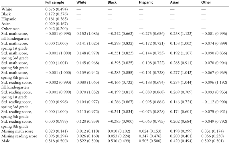
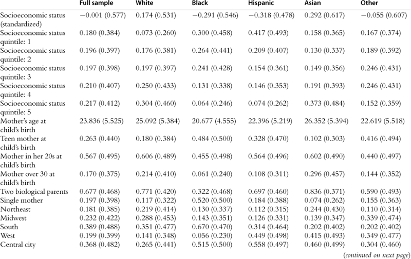
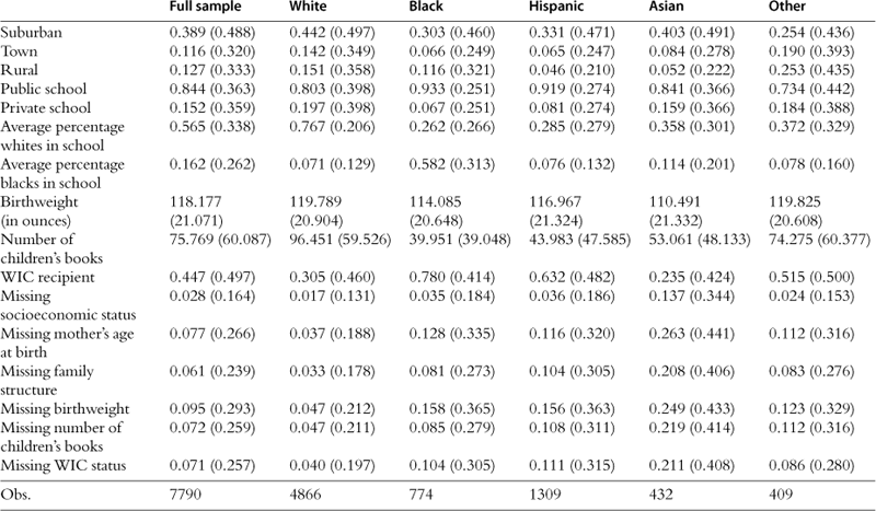
Socioeconomic composite measure
The socioeconomic scale variable (SES) was computed by ECLS at the household level for the set of parents who completed the parent interview in fall kindergarten or spring kindergarten. The SES variable reflects the socioeconomic status of the household at the time of data collection for spring kindergarten. The components used for the creation of SES were: father or male guardian’s education, mother or female guardian’s education, father or male guardian’s occupation, mother or female guardian’s occupation, and household income.
Number of children’s books
Parents or guardians were asked, “How many books does your child have in your home now, including library books?” Answers ranged from 0 to 200.
Child’s age
We used the composite variable child’s age at assessment provided by ECLS. The child’s age was calculated by determining the number of days between the child assessment date and the child’s date of birth. The number was then divided by 30 to calculate the age in months.
Birth weight
Parents were asked how much their child weighed when they were born. We multiplied the number of pounds by 16 and added it to the ounces to calculate birth weight in ounces.
Mother’s age at first birth
Mothers were asked how old they were at the birth of their first child.
A.7 Children of the national longitudinal survey of youth (CNLSY)
There are 11,469 children in the original sample. We drop 2413 children who do not have valid scores for an assessment. We drop 4 more children whose mothers have invalid birth years (before 1957 or after 1964), 459 more children whose mothers have invalid AFQT scores (or whose mothers had recorded problems with the test administration), and 568 more children whose mothers are from the military or low-income white oversamples, for an overall sample of 8025 children.
We define the age group with 5-year-olds as those children between 60 and 71 months old (3375 children). We define the age group with 6–10-year-olds as those children who are between 72 and 119 months old (7699 children). We define the age group with 10–14-year-olds as those children who are between 120 and 179 months old (7107 children). Note that many children have observations in multiple age groups because they participated in multiple assessments.
Income
We construct income as follows: For each child, we look at all of the incomes that the child’s mother had between 1979 and 2006 which are available in the dataset. We use the income that is closest to the assessment year and convert it to 1979 dollars. If two incomes are equally close to the assessment year, then we use the earlier one.
Demographic variables
Free lunch, special education, and private school are defined as follows: The variable is 1 if the child was in the program in either the 1994 or 1995 school survey. The variable is 0 if the child was never in the program and if the child was recorded as not being in the program in the 1994 or 1995 school survey. The variable is missing otherwise.
Test scores
Test scores are standardized within the sample by age group. Mother’s AFQT score is standardized within the sample.
A.8 National assessment of educational progress (NAEP)
All data is derived from the 2007 NAEP data. Note that there is a different sample of students for each of the 4 tests. In the full NAEP sample, there are 191,040 children who took the 4th grade reading test, 197,703 who took the 4th grade math test, 160,674 who took the 8th grade reading test, and 153,027 who took the 8th grade math test. Within the Trial Urban District Assessment (TUDA) subsample, there are 20,352 students who took the 4th grade reading test, 17,110 who took the 8th grade reading test, 21,440 who took the 4th grade math test, and 16,473 who took the 8th grade math test.
Test scores
To calculate the overall test score, we take the mean of the 5 plausible test score values. For analysis that includes the entire NAEP sample, test scores are standardized across the entire sample. For analysis that includes only the district sample, test scores are standardized across the district (TUDA) subsample.
A.9 Chicago public schools
We use Chicago Public Schools (CPS) ISAT test score administrative data from the 2008–09 school year. In our data file, there are 177,001 students with reading scores and 178, 055 students with math scores (grades 3–8). We drop 273 students for whom we are missing race information. This leaves us with 176,767 students with non-missing reading scores and 177,787 students with non-missing math scores.
Demographic variables
We use 4 different CPS administrative files to construct demographic data. These files are the 2009–10 enrollment file, and 2008–09 enrollment file, a file from 2008–09 with records of all students in the school district, and a file from 2008–09 containing records for students in bilingual education. For the demographic variables that should not change over time (race, sex, age), we give use the variables from the 2009–10 enrollment file to construct these and then fill in missing values using the other three files in the order of precedence listed above. For the demographic variables that may vary from year to year (free lunch and ELL status), we use the same process but exclude the 2009–10 enrollment file since it is from a year that is not the same as the year in which the ISAT test score was administered. Note that we include both “free” and “reduced” lunch statuses for our construction of the free lunch variable.
School ID
In order to construct school ID, we use the school ID from the 2008–09 enrollment file but fill in missing values with the 2008–09 with records of all students in the school district. For the purposes of analysis, we assign a common school ID to the 928 students (about 0.5% of the sample) for whom we are still missing school ID information.
Test scores
Illinois Standards Achievement Test (ISAT) scores for math, reading, science, and writing were pulled from a file listing scores for all students in Chicago Public Schools. Eighth graders do not take the science portion of the test and we decided to use only math and reading scores to keep the analysis consistent across districts. ISAT test scores are standardized to have mean 0 and standard deviation 1 within each grade.
A.10 Dallas independent school district
We pull our Dallas TAKS scores from files provided by the Dallas Independent School District (DISD). There are 33,881 students for whom we have non-missing TAKS score data. We use two files to construct grade and school ID information for these students: the 2008–09 DISD enrollment file and the 2008–09 DISD transfers file (containing students who were either not in the school district at the time the enrollment file information was compiled or who ever transferred schools during the school year). We drop 15 students (about 0.04% of the sample) whose grade at the time of the tests cannot be definitively determined either because they skipped a grade during the school year or because their grade levels in the enrollment and transfers files conflict. This leaves us with a sample of 33,866 students in grades 3–5 with non-missing TAKS score data. Within this sample, there are no students with missing race data. This leaves us with 28,126 students in grades 3–5 with non-missing TAKS reading scores and 33,561 students in grades 3–5 with non-missing TAKS math scores.
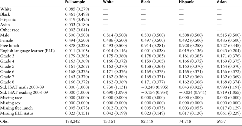
Age
To calculate age in months, we calculate the exact number of days old each student was as of August 25, 2008 (the first day of the 2008–09 school year) and then divide by 30 and round down to the nearest integer number of months.
Demographic variables
In order to construct demographic data, we use the demographic information from the 2008–09 enrollment file. For the race, sex, and age variables, we fill in missing information using the enrollment files from 2002–03 through 2007–08, giving precedence to the most recent files first.
Income
In order to construct the income variable, we use ArcGIS software to map each student’s address from the 2008–09 enrollment file to a 2000 census tract block group. Then we assign each student’s income as the weighted average income of all those who were surveyed in that census tract block group in 2000.
School ID
We construct school ID as follows: For students who attended only one school during the 2008–09 school year, we assign them to that school. For students who attended more than one school according to the transfers file, we assign the school that they attended for the greatest number of days. If a student attended more than one school for equally long numbers of days, we use the school among these with the lowest school identification number.
Test scores
Students in grades three through five take the Texas Assessment of Knowledge and Skills (TAKS). TAKS has a variety of subjects. We use scores from the reading and math sections of this exam. Unlike the Iowa Test of Basic Skills (ITBS) scores, the TAKS data that we have are not grade-equivalent scores. In order to ease interpretation of these scores, we standardize them by, for every subject and year, subtracting the mean and dividing by the standard deviation.
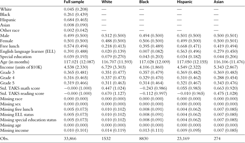
A.11 New york city department of education
We pull our NYC math and ELA scores from NYC Public Schools (NYCPS) test score administrative files. There are 427,688 students (in grades 3–8) with non-missing ELA score data and 435,560 students (in grades 3–8) with non-missing math score data. We drop 1230 students for whom we are missing race information (about 0.3% of the sample). This leaves us with a sample of 426,806 students with non-missing ELA score data and 434,593 students with non-missing math score data.
Age
To calculate age in months, we calculate the exact number of days old each student was as of September 2, 2008 (the first day of the 2008–09 school year) and then divide by 30 and round down to the nearest integer number of months.
Demographic variables
In order to construct demographic data, we use the demographic information from the 2008–09 enrollment file. For the race, sex, and age variables, we fill in missing information using the enrollment files from 2003–04 through 2007–08, giving precedence to the most recent files first.
Income
In order to construct the income variable, we use ArcGIS software to map each student’s address from the 2008–09 enrollment file to a 2000 census tract block group. Then we assign each student’s income as the weighted average income of all those who were surveyed in that census tract block group in 2000.
School ID
We assign school ID for each subject as the school ID recorded in the 2008–09 test score file for that subject. We use Human Resources files provided by NYCPS to link students to their teachers for ELA and math.
Test scores
The New York state math and ELA tests, developed by McGraw-Hill, are high-stakes exams conducted in the winters of third through eighth grades. Students in third, fifth, and seventh grades must score proficient or above on both tests to advance to the next grade. The math test includes questions on number sense and operations, algebra, geometry, measurement, and statistics. Tests in the earlier grades emphasize more basic content such as number sense and operations, while later tests focus on advanced topics such as algebra and geometry. The ELA test is designed to assess students on three learning standards—information and understandings, literary response and expression, and critical analysis and evaluation—and includes multiple-choice and short-response sections based on a reading and listening section, along with a briefediting task.
In our analysis ELA and math scores are standardized by subject and by grade level to have mean 0 and standard deviation 1.
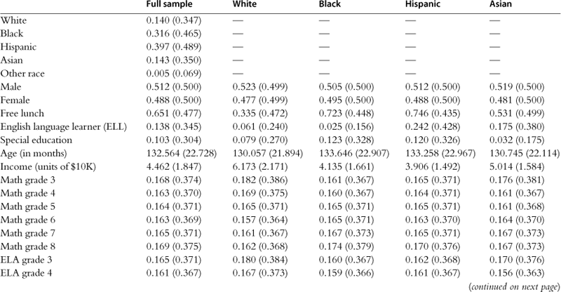
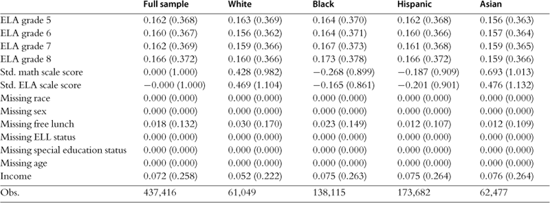
A.12 District data: washington, DC
We pull our DCCAS test scores from DC Public Schools (DCPS) test score administrative files from 2008–09. There are 20,249 students with non-missing reading scores and 20,337 students with non-missing math scores. We drop 6 observations because the students have two observations with conflicting test scores. This leaves us with a sample of 20,243 students with non-missing reading scores and 20,331 students with non-missing math scores, all from grades 3–8 and 10 (the full set of grades for which the DCCAS tests are administered).
Age
To calculate age in months, we calculate the exact number of days old each student was as of August 25, 2008 (the first day of the 2008–09 school year) and then divide by 30 and round down to the nearest integer number of months.
Demographic variables
In order to construct demographic data, we use the demographic information from the 2008–09 enrollment file and use the DCCAS test score file from 2008–09 to fill in missing demographic information. For the race, sex, and age variables, we fill in missing information using the enrollment files from 2005–06 through 2007–08, giving precedence to the most recent files first.
Income
In order to construct the income variable, we use ArcGIS software to map each student’s address from the 2008–09 enrollment file to a 2000 census tract block group. Then we assign each student’s income as the weighted average income of all those who were surveyed in that census tract block group in 2000.
School ID
We assign school ID as the school ID recorded in the 2008–09 DCCAS test score file.
Test scores
The DC CAS is the DC Comprehensive Assessment System and is administered each April to students in grades three through eight as well as tenth graders. It measures knowledge and skills in reading and math. Students in grades four, seven, and ten also take a composition test; students in grades five and eight also take a science test; and students in grades nine through twelve who take biology also take a biology test
DCCAS scores are standardized by subject and by grade level to have mean 0 and standard deviation 1.
A.13 National education longitudinal study of 1988 (NELS)
We use the first three waves (1988, 1990, and 1992) of the NELS panel dataset for our analysis, when respondents were in 8th, 10th, and 12th grade, respectively. There were 19,645 students in the 8th grade cohort, 18,176 students in the 10th grade cohort, and 17,161 students in the 12th grade cohort. We use IRT-estimated number right scores for the analysis. In the base year, there are 23,648 students with non-missing math scores, 23,643 students with non-missing English scores, 23,616 students with non-missing science scores, and 23,525 students with non-missing history scores. In the first follow-up year, there are 17,793 students with non-missing math scores, 17,832 students with non-missing English scores, 17,684 students with non-missing science scores, and 17,591 students with non-missing history scores. In the second follow-up year, there are 14,236 students with non-missing math scores, 14,230 students with non-missing English scores, 14,134 students with non-missing science scores, and 14,063 students with non-missing history scores. If first follow-up and second follow-up scores are missing, we impute them from one another.
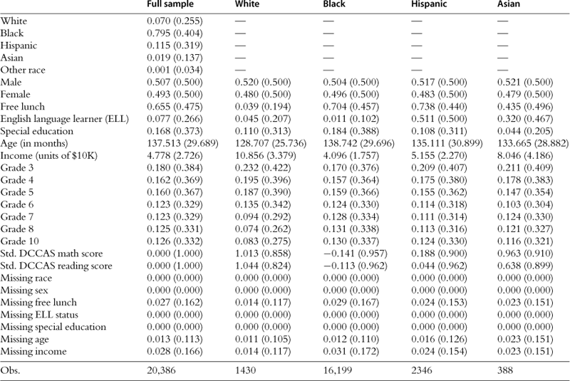
Age
We use birth year and birth month to calculate each student’s age as of September 1988.
Income
The income variable is constructed using the income reported in the base year parent questionnaire. The variable in the dataset categorizes income into different ranges, and our income variable is coded as the midpoint of each range, with the exception of the lowest income category (which corresponds to no income), which we code as $0, and the highest income category (which corresponds to an income of $200,000 or more), which we code as $200,000. We divide income by $10,000.
Parent’s education
Parents’ education refers to the highest level of education obtained by either parent.
School ID
In order to construct the base year school ID, we use the base year school ID variable but supplement it using the student ID when it is missing. The base year school ID is embedded in the student ID as all but the last two digits of the student ID.
Socioeconomic status
We take the SES quartile variable directly from the dataset.
References
1. Abdulkadiroglu Atila, Angrist Joshua, Dynarski Susan, Kane Thomas J, Pathak Parag. Accountability and flexibility in public schools: evidence from Boston’s charters and pilots Working paper no 15549. Cambridge, MA: NBER; 2009.
2. Administration for Children and Families. Preliminary Findings from the Early Head Start Prekindergarten Followup. Washington, DC: US Department of Health and Human Services Report; 2006.
3. Andrews Susan Ring, Blumenthal Janet Berstein, Johnson Dale L, et al. The skills of mothering: a study of parent child development centers. Monographs of the Society for Research in Child Development. 1982;47(6):1–83.
4. Angrist Joshua D, Lang Kevin. Does school integration generate peer effects? Evidence from Boston’s Metco program. The American Economic Review. 2004;94(5):1613–1634.
5. Angrist Joshua D, Dynarski Susan M, Kane Thomas J, Pathak Parag A, Walters Christopher R. Who benefits from KIPP? Working paper no 15740. Cambridge, MA: NBER; 2010.
6. Banks James A. Approaches to multicultural curriculum reform. In: Banks James A, Banks Cherry AM, eds. Multicultural Education: Issues and Perspectives. New York: John Wiley & Sons, Inc., 2001; fourth ed.
7. Banks James A. Cultural Diversity and Education: Foundations, Curriculum, and Teaching. Boston, MA: Pearson Education, Inc., 2006.
8. Barton Paul E. Parsing the achievement gap: baselines for tracking progress. Princeton, NJ: Policy Information Report, Educational Testing Service Policy Information Report; 2003.
9. Bayley Nancy. Comparisons of mental and motor test scores for ages 1 to 15 months by sex, birth order, race, geographical location, and education of parents. Child Development. 1965;36:379–411.
10. Becker Douglas F, Forsyth Robert A. Gender differences in mathematics problem solving and science: a longitudinal analysis. International Journal of Educational Research. 1994;21(4):407–416.
11. Bernstein Lawrence, Dun Rappaport Catherine, Olsho Lauren, Hunt Dana, Levin Magorie, et al. Impact evaluation of the US Department of Education’s Student Mentoring Program: final report. Institute of Education Sciences, Washington, DC: US Department of Education; 2009.
12. Bethel, James, Green, James L., Kalton, Graham, Nord, Christine, 2004. Early childhood longitudinal study, birth cohort (ECLS-B), sampling. Volume 2 of the ECLS-B Methodology Report for the 9-Month Data Collection, 2001–02, US Department of Education, NCES, Washington, DC.
13. Bloom, Dan, Gardenhire-Crooks, Alissa, Mandsager, Conrad, 2009. Reengaging high school dropouts: early results of the National Guard Youth Challenge Program evaluation, MDRC Report, New York.
14. Borman Geoffrey D, Slavin Robert E, Cheung Alan CK, Chamberlain Anne M, Madden Nancy A, Chambers Bette. Final reading outcomes of the national randomized field trial of Success for all. American Educational Research Journal. 2007;44(3):701–731.
15. Bornstein Marc H, Sigman Marian D. Continuity in mental development from infancy. Child Development. 1986;57(2):251–274.
16. Boyd Donald, Grossman Pamela, Lankford Hamilton, Loeb Susanna, Wyckoff James. Teacher preparation and student achievement Working paper no 14314. Cambridge, MA: NBER; 2008.
17. Brooks-Gunn Jeanne, Liaw Fong-ruey, Klebanov Pamela Kato. Effects of early intervention on cognitive function of low birth weight preterm infants. Journal of Pediatrics. 1992;120(3):350–359.
18. Campbell Frances A, Ramey Craig T. Cognitive and school outcomes for high-risk African-American students at Middle Adolescence: positive effects of early intervention. American Educational Research Journal. 1994;32(4):743–772.
19. Campbell Jay R, Hombo Catherine M, Mazzeo John. NAEP 1999 trends in academic progress: three decades of student performance. NCES, Washington, DC: US Department of Education; 2000.
20. Carneiro Pedro, Heckman James. Human capital policy Working paper no 9495. Cambridge, MA: NBER; 2003.
21. Chenoweth Karin. It’s Being Done: Academic Success in Unexpected Schools. Cambridge, MA: Harvard University Press; 2007.
22. Cohen Geoffrey L, Garcia Julio, Purdie-Vaughns Valerie, Apfel Nancy, Brzutoski Patricia. Recursive processes in self-affirmation: intervening to close the minority achievement gap. Science. 2009;324(5925):400–403.
23. Coleman James S, Campbell Ernest Q, Hobson Carol J, et al. Equality of educational opportunity. Washington, DC: US Department of Health, Education, and Welfare, Office of Education; 1966.
24. Congressional Record, No. 11, p. H417 (daily ed. Jan. 27, 2010) (statement of The President).
25. Cook Thomas D, Habib Farah-Naaz, Phillips Meredith, Settersten Richard A, Shagle Shobha C, Degirmencioglu Serdar M. Comer’s School Development Program in Prince George’s county, Maryland: a theory-based evaluation. American Educational Research Journal. 1999;36(3):543–597.
26. Corrin William, Somers Marie-Andree, Kemple James J, Nelson Elizabeth, Sepanik Susan, et al. The enhanced reading opportunities study: findings from the second year of implementation. Washington, DC: US Department of Education, Institute of Education Sciences; 2009.
27. Currie Janet, Thomas Duncan. Does Head Start make a difference? American Economic Review. 1995;85(3):341–364.
28. Curto Vilsa E, Fryer Roland G, Howard Meghan L. It may not take a village: increasing achievement among the poor. Harvard University: Unpublished paper; 2010.
29. Darity Jr. William A, Mason Patrick L. Evidence on discrimination in employment: codes of color, codes of gender. Journal of Economic Perspectives. 1998;12(2):63–90.
30. Datnow Amanda, Park Vicki, Kennedy Brianna. Acting on data: how urban high schools use data to improve instruction. USC Rossier School of Education, Los Angeles: Center on Educational Governance; 2008.
31. Decker Paul, Mayer Daniel, Glazerman Steven. The effects of teach for America on students: findings from a national evaluation. Princeton, NJ: Mathematica Policy Research, Inc., Report; 2004.
32. Dee Thomas. Conditional cash penalties in education: evidence from the learnfare experiment Working paper no 15126. Cambridge, MA: NBER; 2009.
33. Dickens William T, Flynn James R. Heritability estimates versus large environmental effects: the IQ paradox resolved. Psychological Review. 2001;108(2):346–369.
34. Dickens William T, Flynn James R. Black Americans reduce the racial IQ gap: evidence from standardization samples. Psychological Science. 2006;17(10):913–920.
35. Dobbie Will, Fryer Jr Roland G. Are high quality schools enough to close the achievement gap? Evidence from a social experiment in Harlem Working paper no 15473. Cambridge, MA: NBER; 2009.
36. Domina Thurston. Leveling the home advantage: assessing the effectiveness of parental involvement in elementary school. Sociology of Education. 2005;78(3):233–249.
37. Easton John Q, Flinspach Susan Leigh, O’Connor Carla, Paul Mark, Qualls Jesse, Ryan Susan P. Local school council governance: the third year of Chicago school reform. Chicago, IL: Chicago Panel on Public School Policy and Finance; 1993.
38. Farber Henry S, Gibbons Robert. Learning and wage dynamics. Quarterly Journal of Economics. 1996;111(4):1007–1047.
39. Franzini L, Ribble JC, Keddie AM. Understanding the Hispanic paradox. Ethnicity and Disease. 2001;11:496–518.
40. Fryer Roland G, Levitt Steven D. Understanding the black-white test score gap in the first two years of school. Review of Economics and Statistics. 2004;86(2):447–464.
41. Fryer Roland G, Levitt Steven D. The black-white test score gap through third grade. American Law and Economics Review. 2006;8(2):249–281.
42. Fryer Roland G, Levitt Steven D. An empirical analysis of the gender gap in mathematics. American Economic Journal: Applied Economics. 2010;2(2):210–240.
43. Fryer, Roland G., Levitt, Steven D., Testing for racial differences in the mental ability of young children. American Economic Review (forthcoming).
44. Fryer Roland G. Financial incentives and student achievement: evidence from randomized trials. Harvard University: Unpublished paper; 2010.
45. Garber Howard L. The Milwaukee Project: preventing mental retardation in children at risk. Washington, DC: National Institute of Handicapped Research Report; 1988.
46. Garces Eliana, Thomas Duncan, Currie Janet. Longer-term effects of Head Start. American Economic Review. 2002;92(4):999–1012.
47. Garet Michael S, Cronen Stephanie, Eaton Marian, et al. The impact of two professional development interventions on early reading instruction and achievement. Washington, DC: US Department of Education, Institute of Education Sciences; 2008.
48. Goolsbee Austan, Guryan Jonathan. The impact of Internet subsidies in public schools. Review of Economics and Statistics. 2006;88(2):336–347.
49. Gormley Jr. William T, Gayer Ted, Phillips Deborah, Dawson Brittany. The effects of universal Pre-K on cognitive development. Developmental Psychology. 2005;41(6):872–884.
50. Gray Susan W, Klaus Rupert A. The early training project: a seventh-year report. Child Development. 1970;41:909–924.
51. Greene Jay P, Winters Marcus A. Getting ahead by staying behind: an evaluation of Florida’s program to end social promotion. Education Next. 2006;6(2):65–69.
52. Guryan Jonathan. Does money matter? Regression-discontinuity estimates from education finance reform in Massachusetts Working paper no 8269. Cambridge, MA: NBER; 2001.
53. Guskey Thomas R, Gates Sally L. A synthesis of research on group-based mastery learning programs. Chicago, IL: American Educational Research Association Presentation; 1985.
54. Hanushek Eric A, Kain John, Rivkin Steven, Branch Gregory. Charter school quality and parental decision making with school choice Working paper no 11252. Cambridge, MA: NBER; 2005.
55. Hart Betty, Risley Todd R. Meaningful Differences in the Everyday Experience of Young American Children. Baltimore, MD: Brookes; 1995.
56. Hawkins J, David Kosterman, Rick Catalano, Hill Richard F, Karl Abbott G, Robert D. Effects of social development intervention in childhood fifteen years later. Archives of Pediatrics & Adolescent Medicine. 2008;162(12):1133–1141.
57. Heckman James J, Moon Seong Hyeok, Pinto Rodrigo, Savelyev Peter A, Yavitz Adam. The rate of return to the High/Scope Perry Preschool program Working paper no 15471. Cambridge, MA: NBER; 2009.
58. Heckman James J. Detecting discrimination. Journal of Economic Perspectives. 1998;12(2):101–116.
59. Heckman James J. Policies to foster human capital Working paper no 7288. Cambridge, MA: NBER; 1999.
60. Henig Jeffrey R, Rich Wilbur C. Mayors in the Middle: Politics, Race, and Mayoral Control of Urban Schools. Princeton, NJ: Princeton University Press; 2004.
61. Hoxby Caroline M, Murarka Sonali. Charter schools in New York City: who enrolls and how they affect their students’ achievement Working paper no 14852. Cambridge, MA: NBER; 2009.
62. Hoxby Caroline M, Rockoff Jonah E. The impact of charter schools on student achievement. Harvard University: Unpublished paper; 2004.
63. Jacob Brian A, Lefgren Lars. Remedial education and student achievement: a regression- discontinuity analysis. Review of Economics and Statistics. 2004;86(1):226–244.
64. Jacob Brian A, Ludwig Jens. Improving educational outcomes for poor children Working paper no 14550. Cambridge, MA: NBER; 2008.
65. Jacob Brian A. Public housing, housing vouchers, and student achievement: evidence from public housing demolitions in Chicago. American Economic Review. 2004;94(1):233–258.
66. Jacob Brian A. Accountability, incentives and behavior: the impact of high-stakes testing in the Chicago public schools. Journal of Public Economics. 2005;89:761–796.
67. James-Burdumy Susanne, Mansfield Wendy, Deke John, et al. Effectiveness of Selected Reading Comprehension Interventions: Impacts on a First Cohort of Fifth-Grade Students. Institute of Education Sciences, Washington, DC: US Department of Education; 2009.
68. Jencks Christopher. Racial bias in testing. In: Jencks Christopher, Phillips Meredith, eds. The Black-White Test Score Gap. Washington, DC: The Brookings Institution Press; 1998;55–85.
69. Jensen Arthur R. Educability and Group Differences. New York: The Free Press; 1973.
70. Jensen Arthur R. Genetic and behavioral effects of nonrandom mating. In: Noble Clyde E, ed. Human Variation: Biogenetics of Age, Race, and Sex. New York: Academic Press; 1978.
71. Jensen Arthur R. The G Factor: The Science of Mental Ability. Westport, CT: Praeger; 1998.
72. Kane Thomas J, Rockoff Jonah E, Staiger Douglas O. What does certification tell us about teacher effectiveness? Evidence from New York City Working paper no 12155. Cambridge, MA: NBER; 2008.
73. Kemple James J. Career academies: long-term impacts on labor market outcomes, educational attainment, and transitions to adulthood. New York: MDRC Report; 2008.
74. Kemple James J, Herlihy Corinne M, Smith Thomas J. Making progress toward graduation: evidence from the talent development high school model. New York: MDRC Report; 2005.
75. Klebanov Pamelo Kato. Does neighborhood and family poverty affect mothers’ parenting, mental health, and social Support? Journal of Marriage and Family. 1994;56(2):441–455.
76. Kling Jeffrey R, Liebman Jeffrey B, Katz Lawrence F. Experimental analysis of neighborhood effects. Econometrica. 2007;75(1):83–119.
77. Knight Jim (Ed). Coaching: Approaches and Perspectives. Thousand Oaks, CA: Corwin Press; 2009.
78. Krieger Nancy, Sidney Stephen. Racial discrimination and blood pressure: the CARDIA study of young black and white adults. American Journal of Public Health. 1996;86(10):1370–1378.
79. Krueger Alan B. Experimental estimates of education production functions. Quarterly Journal of Economics. 1999;114(2):497–532.
80. Krueger Alan B, Whitmore Diane. Would smaller classes help close the black white achievement gap? Working paper no 451. Princeton University: Industrial Relations Section; 2001.
81. Krueger Alan B, Zhu Pei. Another look at the New York City school voucher experiment Working paper no 9418. Cambridge, MA: NBER; 2002.
82. Lally J Ronald, Mangione Peter L, Honig Alice S. The Syracuse University Family Development Research Program: Long-Range Impact of an Early Intervention with Low-Income Children and their Families. San Francisco, CA: Center for Child & Family Studies, Far West Laboratory for Educational Research & Development; 1987.
83. Lang Kevin, Manove Michael. Education and labor-market discrimination Working paper no 12257. Cambridge, MA: NBER; 2006.
84. Lauer Patricia A, Akiba Motoko, Wilkerson Stephanie B, Apthorp Helen S, Snow David, Martin-Glenn Mya L. Out-of-school-time programs: a meta-analysis of effects for at-risk students. Review of Educational Research. 2006;76(2):275–313.
85. Levin Jessica, Quinn Meredith. Missed opportunities: how we keep high-quality teachers out of urban classrooms. The New Teacher Project: Unpublished paper; 2003.
86. Lewis Michael, McGurk Harry. Evaluation of infant intelligence. Science. 1972;178(December 15):1174–1177.
87. List John A. The behavioralist meets the market: measuring social preferences and reputation effects in actual transactions Working paper no 11616. Cambridge, MA: NBER; 2005.
88. Lochner Lance, Moretti Enrico. The effect of education on crime: evidence from prison inmates, arrests, and self-reports. American Economic Review. 2004;94(1):155–189.
89. Marlow Michael L. Spending, school structure, and public education quality: evidence from California. Economics of Education Review. 2000;19(1):89–106.
90. McCall Robert B, Carriger Michael S. A meta-analysis of infant habituation and recognition memory performance as predictors of later IQ. Child Development. 1993;64(1):57–79.
91. Morrow-Howell Nancy, Jonson-Reid Melissa, McCrary Stacey, Lee YungSoo, Spitznagel Ed. Evaluation of experience corps: student reading outcomes. St. Louis, MO: Unpublished paper, Center for Social Development, George Warren Brown School of Social Work, Washington University; 2009.
92. Neal Derek A, Johnson William R. The role of premarket factors in black-white wage differences. Journal of Political Economy. 1996;104(5):869–895.
93. Neal Derek. Why has black-white skill convergence stopped? Working paper no. NBER, Cambridge, MA: 11090; 2005.
94. Neisser Ulric, Boodoo Gwyneth, Bouchard Jr. Thomas J, et al. Intelligence: knowns and unknowns. American Psychologist. 1996;51(2):77–101.
95. Nelson Charles A. The neurobiological bases of early intervention. In: Shonkoff Jack P, Meisels Samuel J, eds. Handbook of Early Childhood Intervention. New York: Cambridge University Press; 2000.
96. Nisbett Richard E. Race, genetics, and IQ. In: Jencks Christopher, Phillips Meredith, eds. The Black-White Test Score Gap. Washington, DC: The Brookings Institution Press; 1998;86–102.
97. Niswander KR, Gordon M. The Women and their Pregnancies: The Collaborative Perinatal Study of the National Institute of Neurological Diseases and Stroke. Washington, DC: US Government Print Office; 1972.
98. Nord Christine, Andreassen Carol, Branden Laura, et al. Early Childhood Longitudinal Study, Birth cohort (ECLS-B), user’s manual for the ECLS-B nine-month public-use data file and electronic code book. NCES, Washington, DC: US Department of Education; 2005.
99. Nye KE. The effect of school size and the interaction of school size and class type on selective student achievement measures in Tennessee elementary schools. University of Tennessee, Knoxville, TN: Unpublished doctoral dissertation; 1995.
100. Olds David, Henderson Charles R, Cole Robert, et al. Long-term effects of nurse home visitation on children’s criminal and antisocial behavior. Journal of the American Medical Association. 1998;280(14):1238–1244.
101. Olds David L, Robinson JoAnn, O’Brien Ruth, et al. Home visiting by paraprofessionals and by nurses: a randomized, controlled trial. Pediatrics. 2002;110(3):486–496.
102. O’Neill June. The role of human capital in earnings differences between black and white men. Journal of Economic Perspectives. 1990;4(4):25–45.
103. r Devah. The use of field experiments for studies of employment discrimination: contributions, critiques, and directions for the future. Annals of the American Academy of Political and Social Science. 2007;609(1):104–133.
104. Phillips Meredith, Brooks-Gunn Jeanne, Duncan Greg J, Klebanov Pamela, Crane Jonathan. Family background, parenting practices, and the black-white test score gap. In: Jencks Christopher, Phillips Meredith, eds. The Black-White Test Score Gap. Washington, DC: The Brookings Institution Press; 1998a;103–147.
105. Phillips Meredith, Crouse James, Ralph John. Does the black-white test score gap widen after children enter school? In: Jencks Christopher, Phillips Meredith, eds. The Black-White Test Score Gap. Washington, DC: The Brookings Institution Press; 1998b;229–272.
106. Plomin Robert, DeFries John C, McClearn Gerald E, McGuffin Peter. Behavioral Genetics. New York: Worth; 2000.
107. Podgursky Michael J, Springer Matthew G. Teacher performance pay: a review. Journal of Policy Analysis and Management. 2007;26(4):909–949.
108. Protheroe Nancy J, Barsdate Kelly J. Culturally Sensitive Instruction and Student Learning. Arlington, VA: Educational Research Center; 1991.
109. Puma Michael, Bell Stephen, Cook Ronna, Heid Camilla, Lopez Michael, et al. Head Start Impact Study: First Year Findings. Washington, DC: US Department of Health and Human Services; 2005.
110. Puma Michael, Bell Stephen, Cook Ronna, Heid Camilla, et al. Head Start Impact Study: Final Report. Washington, DC: US Department of Health and Human Services; 2010.
111. Reuter EB. Racial theory. American Journal of Sociology. 1945;50(6):452–461.
112. Rock Donald A, Stenner Jackson. Assessment issues in the testing of children at school entry. The Future of Children. 2005;15(1):15–34.
113. Rockoff Jonah E. The impact of individual teachers on student achievement: evidence from panel data. American Economic Review. 2004;94(2):247–252.
114. Rockoff Jonah E. Does mentoring reduce turnover and improve skills of new employees? Evidence from teachers in New York City Working paper no 13868. Cambridge, MA: NBER; 2008.
115. Rouse Cecilia E, Krueger Alan B. Putting computerized instruction to the test: a randomized evaluation of a ‘scientifically based’ reading program. Economics of Education Review. 2004;23(4):323–338.
116. Rushton J Philippe, Jensen Arthur. Thirty years of research on race differences in cognitive ability. Psychology, Public Policy, and Law. 2005;11(2):235–294.
117. Rushton J Philippe. Race and crime: international data for 1989–1990. Psychological Reports. 1995;76(1):307–312.
118. Sanbonmatsu Lisa, Kling Jeffrey R, Duncan Greg J, Brooks-Gunn Jeanne. Neighborhoods and academic achievement: results from the moving to opportunity experiment. The Journal of Human Resources. 2006;41(4):649–691.
119. Schanzenbach Diane Whitmore. What have researchers learned from project STAR? Brookings Papers on Education Policy 2006/07: 2007;205–228.
120. Schultz T Paul, Strauss John. Handbook of Development Economics, vol 4. Amsterdam, New York: North-Holland; 2008.
121. Schweinhart Lawrence J, Barnes Helen V, Weikart David P. Significant benefits: the High/Scope Perry Preschool study through age 27. Ypsilanti, MI: High Scope Press; 1993.
122. Shapka Jennifer D, Keating Daniel P. Effects of a girls-only curriculum during adolescence: performance, persistence, and engagement in mathematics and science. American Educational Research Journal. 2003;40(4):929–960.
123. Shonkoff Jack P. A promising opportunity for developmental and behavioral pediatrics at the interface of neuroscience, psychology, and social policy: remarks on receiving the 2005 C. Anderson Aldrich Award Pediatrics. 2006;118:2187–2191.
124. Shukla S. Priorities in educational policy. Economic and Political Weekly. 1971;6(30–32):1649–1651 1653–1654.
125. Taggart Robert. Quantum Opportunity Program Opportunities. Philadelphia, PA: Industrialization Center of America; 1995.
126. Thernstrom Abigail. The drive for racially inclusive schools. Annals of the American Academy of Political and Social Science. 1992;523:131–143.
127. Thompson Ross A. The legacy of early achievements. Child Development. 2000;71(1):145–152.
128. Turney Kristin, Edin Kathryn, Clampet-Lundquist Susan, Kling Jeffrey R, Duncan Greg J. Neighborhood effects on barriers to employment: results from a randomized housing mobility experiment in Baltimore. Brookings-Wharton Papers on Urban Affairs. 2006;2006:137–187.
129. Wagner Mary M, Clayton Serena L. The parents as teachers program: results from two demonstrations. The Future of Children. 1999;9(1):91–115.
130. Walker Gary, Vilella-Velez Frances. Anatomy of a Demonstration: The Summer Training and Education Program (STEP) from Pilot through Replication and Postprogram Impacts. Philadelphia, PA: Public/Private Ventures; 1992.
131. Wigdor Alexandra K, Green Bert F. Performance Assessment for the Workplace, vol 1. Washington, DC: National Academies Press; 1991.
132. Wilson William Julius. More than Just Race: Being Black and Poor in the Inner City (Issues of Our Time). New York: W.W. Norton & Company; 2010.
133. Wong Kenneth L, Shen Francis X. Do school district takeovers work? Assessing the effectiveness of city and state takeovers as school reform strategy. State Education Standard. 2002;3(2):19–23.
134. Wong Kenneth L, Shen Francis X. When mayors lead urban schools: assessing the effects of takeover. In: Howell William G, ed. Beseiged: School Boards and the Future of Education Politics. Washington, DC: The Brookings Institution Press; 2005;81–101.
135. Yeates Keith Owen, MacPhee David, Campbell Frances A, Ramey Craig T. Maternal IQ and home environment as determinants of early childhood intellectual competence: a developmental analysis. Developmental Psychology. 1983;19(5):731–739.
136. Ziedenberg Jason, Schiraldi Vincent. Cellblocks or classrooms? The funding of higher education and corrections and its impact on African American men. Justice Policy Institute: Unpublished paper; 2002.
55Thanks to Josh Angrist for providing his data to construct this figure.
1I am enormously grateful to Lawrence Katz, Steven Levitt, Derek Neal, William Julius Wilson and numerous other colleagues whose ideas and collaborative work fill this chapter. Vilsa E. Curto and Meghan L. Howard provided truly exceptional research assistance. Support from the Education Innovation Laboratory at Harvard University (EdLabs), is gratefully acknowledged.
2The Hispanic-white life expectancy gap actually favors Hispanics in the United States. This is often referred to as the “Hispanic Paradox” (Franzini et al., 2001).
3List (2005), which examines whether social preferences impact outcomes in the actual market through field experiments in the sportscard market, is a notable exception.
4For details on the treatment effects of these programs, see Jacob and Ludwig (2008), Guskey and Gates (1985), and Fryer (2010).
5Lang and Manove (2006) show that including years of schooling in the Neal and Johnson (1996) specification causes the gap to increase—arguing that when one controls for AFQT performance, blacks have higher educational attainment than whites and that the labor market discriminates against blacks by not financially rewarding them for their greater education.
6Summary statistics for NLSY79 are displayed, by race, in Table A.1.
7This may be due, in part, to differential selection out of the labor market between black and white women. See Neal (2005) for a detailed account of this.
8Summary statistics for NLSY97 are displayed, by race, in Table A.2.
9Lochner and Moretti (2004) use a similar approach to determine incarceration rates, using type of residence in Census data and in the NLSY79.
10We focus on the estimates from NLSY79 because we have many more years of observations for these individuals than for those in the NLSY97, which gives us a more accurate picture of incarceration.
11There are two reasons for this. First, the 1976 College & Beyond cohort can be reasonably compared to the NLSY79 cohort because they are all born within a seven-year period. Second, there are issues with using either the 1951 or the 1989 data. The 1951 cohort presents issues of selection bias—black students who entered top colleges in this year were too few in number and those who did were likely to be incredibly motivated and intelligent students, in comparison to both their non-college-going black peers and their white classmates. The 1989 cohort is problematic because the available wage data for that cohort was obtained when that cohort was still quite young. Wage variance is likely to increase a great deal beyond the levels observed in the available wage data. Additionally, some individuals who have high expected earnings were pursuing graduate degrees at the time wage data were gathered, artificially depressing their observed wages.
12Ninety-two percent of the sample has valid SAT scores.
13Individuals in the wage range “less than $1000” are excluded from the analysis as they cannot have made this wage as full-time workers and therefore should not be compared to the rest of the sample.
14A measure of current unemployment for the individuals surveyed was also created. However, only 39 out of 19,257 with valid answers as to employment status could be classified as unemployed, making an analysis of unemployment by race infeasible. Although 1876 reported that they were not currently working for reasons other than retirement, the vast majority of these individuals were out of the labor force rather than unemployed. More details on this variable can be found in the data appendix.
15The SAT is presently called the SAT Reasoning Test and the letters “SAT” no longer stand for anything. At the time these SAT scores were gathered, however, the test was officially called the “Scholastic Aptitude Test” and was believed to function as a valid intelligence test. The test also had a substantially different format and included a different range of question types.
16This argument requires an important leap of faith. We have demonstrated that educational achievement is correlated with better economic and social outcomes, but we have not proven that this relationship is causal. We will come back to this in the conclusion.
17Some scholars have argued that the combination of high heritability of innate ability (typically above 0.6 for adults, but somewhat lower for children, e. g., Neisser et al. (1996) or Plomin et al. (2000), and persistent racial gaps in test scores is evidence of genetic differences across races (Jensen, 1973,1998; Rushton and Jensen, 2005). As Nisbett (1998) and Phillips et al. (1998a,b) argue, however, the fact that blacks, whites, and Asians grow up in systematically different physical and social environments makes it difficult to draw strong, causal, genetically-based conclusions.
18This analysis is a replication and extension of Bayley (1965) and Fryer and Levitt (2004).
19For more information on the coding of these variables, see the data appendix.
20In ECLS, each of the 13 regions was staffed by one field supervisor and between 14 and 19 interviewers, for a total of 256 field staff (243 interviewers), who conducted an average of 42 child assessments each. The number of interviews per interviewer ranges from 1 to 156. Almost all interviewers assessed children from different races (Bethel et al., 2004). There are 184 interviewers in CPP for eight-month-olds, 305 for four-year-olds, and 217 for seven-year-olds. In the CPP, there are many interviewers for whom virtually all of the children assessed were of the same race.
21Because the age at which the test is taken is such an important determinant of test performance, we include separate indicators for months of age in our specification.
22It should also be noted that in the CPP dataset, there is not a single SES measure, but the set of variables including parental education, parental occupation, and family income provides a rich proxy for socioeconomic status.
23Nonetheless, Lewis and McGurk (1972) are pessimistic about the generalizability of these infant test scores. Work focusing on infant attention and habituation is also predictive of future test scores (e. g., Bornstein and Sigman, 1986; McCall and Carriger, 1993), but unfortunately our data do not include such information.
24It is important to note that substantial uncertainty underlies these correlations, which are based on a small number of studies carried out on a non-representative sample.
25Allowing for an individual’s environment to be positively correlated at different points in time causes this simple model to show even greater divergence from what is observed in the data. We relax the assumption that environment is not correlated across ages for an individual when we introduce a correlation between parental test scores and the child’s environment below.
26As noted below, factors such as assortative mating can cause that correlation to be higher.
27Note that the racial gap at age seven is based on earlier CPP data. The evidence suggests that racial gaps have diminished over time (Dickens and Flynn, 2006). Thus, a value of 0.854 in Eq. (7) may be too large. The only implication this has for solving our model is to reduce the black-white differences in environment that are necessary to close the model. We use the raw racial gaps in this analysis, rather than the estimates controlling for covariates, because our goal in this section is to decompose the differences into those driven by genes versus environments. Many of the covariates included in our specifications could be operating through either of those channels.
28A third class of models that we explored has multiple dimensions of intelligence (e. g., lower-order and higher-order thinking) that are weighted differently by tests administered to babies versus older children. We have not been able to make such a model consistent with the observed correlations without introducing either assortative mating or allowing the mother’s test score to influence the child’s environment.
29The correlation of 0.5 can be derived as follows. Let G = 0.5G(M) + 0.5G(F). Taking the correlation of both sides with respect to G(M) and assuming unit variance, corr(G, G(M)) = 0.76 only if corr(G(M), G(F)) = 0.5.
30Allowing black babies to have worse environments makes the implied racial gap in G even smaller.
31Estimates from Fryer and Levitt (2004) on racial differences in achievement when black, white, Asian, and Hispanic students enter kindergarten, along with the assortative mating model above, imply that even smaller differences in environment explain later test scores.
32Fryer and Levitt (2004) find a 0.75 standard deviation difference between blacks and whites in socioeconomic status, a 0.83 standard deviation gap in the number of children’s books in the home, a 1.30 standard deviation difference in female-headed households, a 1.51 standard deviation difference in whether or not one feels safe in their neighborhood, a 1.5 standard deviation difference in the percentage of kids in their school who participate in the free lunch program, and a 1.31 difference in the amount of loitering reported around the school by non-students. All estimates are derived by taking the difference in the mean of a variable between blacks and whites and dividing by the standard deviation for whites. The socioeconomic composite measure contains parental income, education, and occupation.
33See Carneiro and Heckman (2003) for a nice review of policies to foster human capital.
34Local Head Start agencies are able to extend coverage to those meeting other eligibility criteria, such as those with disabilities and those whose families report income between 100 and 130% of the federal poverty level.
35Students not chosen by lottery to participate in Head Start were not precluded from attending other high-quality early childhood centers. Roughly ninety percent of the treatment sample and forty-three percent of the control sample attended center-based care.
36The Early Head Start program, established in 1995 to provide community-based supplemental services to low-income families with infants and toddlers, has similar effects (Administration for Children and Families, 2006).
37Researchers consider a variety of outcomes in determining the monetary value of the benefits of such programs, including the program’s impact on need for special education services, grade retention, incarceration rates, and wages. Heckman et al. (2009) estimate that the long-term return on investment of the Perry Preschool program is between seven and ten percent.
38A more detailed description of each of the variables used is provided in the data appendix.
39Including all the values of these variables from each survey or only those in the relevant years does not alter the results.
40The results above are not likely a consequence of the particular testing instrument used. If one substitutes the teachers’ assessment of the student’s ability as the dependent variable, virtually identical results emerge. Results are available from the author upon request.
41Hispanics seem to increase their position relative to whites in states where English proficiency is known to be a problem (Arizona, California, and Texas).
42One interesting caveat: Hispanics are also less likely to participate in preschool, which could explain their poor initial scores and positive trajectory. However, including controls for the type of program/care children have prior to entering kindergarten does nothing to explain why Hispanics gain ground.
43Using the full eighth grade test reduces the magnitude of losing ground by roughly half, but the general patterns are the same.
44Results from analysis of the Reading Comprehension assessment are qualitatively very similar to results from using the Reading Recognition assessment and are available from the author upon request.
45This corresponds, roughly, to kindergarten entry through ninth grade. To avoid complications due to potential differences in grade retention by race, we analyze CNLSY data by age.
46Similar results are obtained from the National Longitudinal Survey of Adolescent Health (Add Health)—a nationally representative sample of over 90,000 students in grades six through twelve. We chose NELS because it contains tests on four subject areas. Add Health only contains the results from the Peabody Picture Vocabulary Test. Results from Add Health are available from the author upon request.
47This list was generated by typing in “school-aged interventions” into Google Scholar, National Bureau of Economic Research, and JSTOR. From the (much larger) original list, we narrowed our focus to those programs that contained credible identification.
48Individual schools are first selected for participation in NAEP in order to ensure that the assessments are nationally representative, and then students are randomly selected from within those schools. Both schools and students have the option to not participate in the assessments. Tests are given in multiple subject areas in a given school in one sitting, with different students taking different assessments. Assessments are conducted between the last week of January and the first week in March every year. The same assessment is given to all students within a subject and a grade during a given administration.
49The debate over communities or schools often seems to treat these approaches as mutually exclusive, evaluating policies that change one aspect of the schools or a student’s learning environment. This approach is potentially informative on the various partial derivatives of the educational production function but is uninformative on the net effect of many simultaneous changes. The educational production function may, for example, exhibit either positive or negative interactions with respect to various reforms. Smaller classes and more time-on-task matter more (or less) if the student has good teachers; good teachers may matter more (or less) if the student has a good out-of-school environment, and so on.
50This is similar in magnitude to the math racial achievement gap in nationally representative samples [0.082 in Fryer and Levitt (2006) and 0.763 in Campbell et al. (2000)].
51This is smaller than the reading racial achievement gap in some nationally representative samples [0.771 in Fryer and Levitt (2006) and 0.960 in Campbell et al. (2000)].
52Interventions in education often have larger impacts on math scores compared to reading or ELA scores (Decker et al., 2004; Rockoff, 2004; Jacob, 2005). This may be because it is relatively easier to teach math skills, or because reading skills are more likely to be learned outside of school. Another explanation is that language and vocabulary skills may develop early in life, making it difficult to impact reading scores in adolescence (Hart and Risley, 1995; Nelson, 2000).
53On the New York state assessments in the 2008–09 school year, KIPP charter schools had student pass rates that were at least as high as those at the HCZ Promise Academy. This information can be accessed through the New York State Report Cards at https://www.nystart.gov/publicweb/CharterSchool.do?year=2008.
54However, the typical middle school applicant in Abdulkadiroglu et al (2009) starts 0 286 and 0 348 standard deviations higher in fourth grade math and reading than the typical Boston student, and the typical high school applicant starts 0. 380 standard deviations higher on both eighth grade math and reading tests.
56See Curto et al. (2010) for more discussion on caveats to taking strategies from charter schools to scale.
57In cases where there are missing values for another of these covariates, we set these missing observations equal to zero and add an indicator variable to the specification equal to one if the observation is missing and equal to zero otherwise. We obtain similar results for the first wave when we include all children with an initial test score, including those who subsequently are not tested.
58A comparison of the ECLS-B sample characteristics with known national samples, such as the US Census and the Center for Disease Control’s Vital Statistics, confirms that the sample characteristics closely match the national average.
59See Nord et al. (2005) for further details.
60Detailed information on the selection methods and sampling frame from each institution can be found in Niswander and Gordon (1972). Over 400 publications have emanated from the CPP; for a bibliography, see http://www.niehs.nih.gov/research/atniehs/labs/epi/studies/dde/biblio.cfm. The most relevant of these papers is Bayley (1965), which, like our reanalysis, finds no racial test score gaps among infants.
61Analyzing each wave of the data’s test scores, not requiring that a student have all three scores, yields similar results.
62It must be noted, however, that there are a great deal of missing data on covariates in CPP; in some cases more than half of the sample has missing values. We include indicator variables for missing values for each covariate in the analysis.
63A “general knowledge” exam was also administered. The general knowledge test is designed to capture “children’s knowledge and understanding of the social, physical, and natural world and their ability to draw inferences and comprehend implications.” We limit the analysis to the math and reading scores, primarily because of the comparability of these test scores to past research in the area. In addition, there appear to be some peculiarities in the results of the general knowledge exam. See Rock and Stenner (2005) for a more detailed comparison of ECLS to previous testing instruments.
64For more detail on the process used to generate the IRT scores, see Chapter 3 of the ECLS-K Users Guide. Our results are not sensitive to normalizing the IRT scores to have a mean of zero and standard deviation of one.
65Because of the complex manner in which the ECLS-K sample is drawn, different weights are suggested by the providers of the data depending on the set of variables used (BYPW0). We utilize the weights recommended for making longitudinal comparisons. None of our findings are sensitive to other choices of weights, or not weighting at all.