
Imperfect Competition in the Labor Market
Manning Alan1, Centre for Economic Performance, London School of Economics, Houghton Street, London WC2A 2AE
Abstract
It is increasingly recognized that labor markets are pervasively imperfectly competitive, that there are rents to the employment relationship for both worker and employer. This chapter considers why it is sensible to think of labor market as imperfectly competitive, reviews estimates on the size of rents, theories of and evidence on the distribution of rents between worker and employer, and the areas of labor economics where a perspective derived from imperfect competition makes a substantial difference to thought.
Keywords
Imperfect competition; Labor markets; Rents; Search; Matching; Monopsony
Introduction
In recent years, it has been increasingly recognized that many aspects of labor markets are best analyzed from the perspective that there is some degree of imperfect competition. At its most general, “imperfect competition” should be taken to mean that employer or worker or both get some rents from an existing employment relationship. If an employer gets rents, then this means that the employer will be worse off if a worker leaves i.e. the marginal product is above the wage and worker replacement is costly. If a worker gets rents then this means that the loss of the current job makes the worker worse off—an identical job cannot be found at zero cost. If labor markets are perfectly competitive then an employer can find any number of equally productive workers at the prevailing market wage so that a worker who left could be costlessly replaced by an identical worker paid the same wage. And a worker who lost their job could immediately find another identical employer paying the same wage so would not suffer losses.
A good reason for thinking that there are rents in the employment relationship is that people think jobs are a “big deal”. For example, when asked open-ended questions about the most important events in their life over the past year, employment-related events (got job, lost job, got promoted) come second after “family” events (births, marriages, divorces and death)—see Table 1 for some British evidence on this. This evidence resonates with personal experience and with more formal evidence—for example, the studies of Jacobson et al. (1993) and Von Wachter, Manchester and Song (2009) all suggest substantial costs of job loss. And classic studies like Oi (1962) suggest non-trivial costs of worker replacement.
Table 1
Self-reported important life events in past year: UK data.
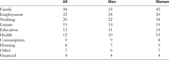
Source: British household panel study.
This chapter reviews some recent developments in thinking about imperfect competition in labor markets. The plan is as follows. The next section outlines the main sources of rents in the employment relationship. The second section discusses some estimates of the size of rents in the employment relationship. The third section then consider theoretical models of how the rents in the employment relationship are split between worker and employer (the question of wage determination) and the fourth section considers evidence on rent-splitting. I argue that this all adds up to a persuasive view that imperfect competition is pervasive in labor markets. But, up to this point, we have not considered the “so what” question—how does the perspective of imperfect competition alter our views on substantive labor market issues?—that is the subject of the fifth section. The sixth section then reviews a number of classic topics in labor economics—the law of one wage, the effect of regulation, the gender pay gap, human capital accumulation and economic geography—where the perspective of imperfect competition can be shown to make a difference.
This chapter is rather different in style from other excellent surveys of this area (e.g. Rogerson et al., 2005 or Mortensen and Pissarides, 1999 or Mortensen, 1986). Much work in this area is phrased in terms of canonical models—one might mention the search and matching models of Pissarides (1985, 2000) or Mortensen and Pissarides (1994) or the wage-posting model of Burdett and Mortensen (1998). New developments are often thought of as departures from these canonical models. Although the use of very particular models encourages precise thinking, that precision relates to the models and not the world and can easily become spurious precision when the models are very abstract with assumptions designed more for analytical tractability than realism. So, a model-based approach to the topic is not always helpful and this survey is based on the beliefthat it can be useful to think in very broad terms about general principles and that one can say useful things without having to couch them in a complete but necessarily very particular model.
1 The sources of imperfect competition
As will be discussed below there are different ways in which economists have sought to explain why there are rents in the employment relationship. This section will argue they are best understood as having a common theme—that, from the worker perspective, it takes time and/or money to find another employer who is a perfect substitute for the current one and that, from an employer perspective, it is costly to find another worker who is a perfect substitute for the current one. And, that, taken individually, these explanations of the sources of rents often do not seem particularly plausible but, taken together, they add up to a convincing description of the labor market.
1.1 Frictions and idiosyncracies
First, consider search models (for relatively recent reviews see Mortensen and Pissarides, 1999; Rogerson et al., 2005). In these models it is assumed that it takes time for employers to be matched with workers because workers’ information about the labor market is imperfect (an idea first put forward by Stigler, 1961, 1962)—in some versions, the job offer arrival rate can be influenced by the expenditure of time and/or money (see Section 2.2.1 below for such a model). These models have become the workhorse model in much of macroeconomics (see Rogerson and Shimer, 2011) because one cannot otherwise explain the dynamics of unemployment. But, taken literally, this model is not very plausible. It is not hard to find an employer—I can probably see 10 from my office window. But, what is hard is to find an employer who is currently recruiting2 who is the same as my current one i.e. a perfect substitute for my current job. This is because there is a considerable idiosyncratic component to employers across a vast multitude of dimensions that workers care about. This idiosyncratic component might come from non-monetary aspects of the job (e.g. one employer has a nice boss, another a nasty one, one has convenient hours, another does not) or from differences in commuting distances or from many other sources. A good analogy is our view of the heavens: the stars appear close together but this is an illusion caused by projecting three dimensions onto two. Neglecting the multitude of dimensions along which employers differ that matter to workers will seriously overestimate our impression of the extent to which jobs are perfect substitutes for each other from the perspective of workers.
One other commonly given explanation for why there may be rents in the employment relationship is “specific human capital”. Although this is normally thought of as distinct from the reasons given above, it is better thought of as another way in which employers may not be perfect substitutes for each other—in this case in terms of the quality of the match or the marginal product of the worker. This comes out clearly in the discussion of specific human capital provided by Lazear (2003). He struggles with the problem of what exactly are specific skills, coming up with the answer that “it is difficult to generate convincing examples where the firm-specific component [of productivity] approaches the general component”. He goes on to argue that all skills are general skills but that different employers vary in how important those skills are in their particular situation. So, a worker with a particular package of general skills will not be faced with a large number of employers requiring exactly that package. As Lazear (2003, p. 2) makes clear, this relies on employers being thin on the ground otherwise a large supply of employers demanding exactly your mix of skills would be available and the market would be perfectly competitive. Again, it is the lack of availability of employers who are perfect substitutes that can be thought of as the source of the rents.
A key and eminently sensible idea in the specific human capital literature originating in Becker (1993) is that specific human capital accumulates over time. This means that rents in the employment relationship are likely to be higher for those workers who have been in their current job for a long time—very few labor economists would dissent from this position. The very fact that we turn up to the same employer day after day strongly suggests there are some rents from that relationship. More controversial is whether, on a worker’s first day in the job, there are already rents because the employer has paid something to hire them and the worker could not get another equivalent job immediately. This paper is predicated on the view that there are rents from the first day3 – that the worker would be disappointed if they turned up for work to be told there was no longer a need for them and that the employer would be irritated if the new hire does not turn up on the first morning.
One interesting question to think about is whether the rapid decline in the costs of supplying and acquiring information associated with the Internet is going to make labor markets more like the competitive ideal in the future than the past. There is no doubt that the Internet (and earlier communication technologies) have transformed job search. In late 19th century London an unemployed worker would have trudged from employer to employer, knocking on doors and enquiring whether there were any vacancies, often spending the whole day on it and walking many miles. In contrast, a worker today can, with access to the Internet, find out about job opportunities throughout the globe. Using the Internet as a method of job search has rapidly become near-universal. For example, in the UK Labour Force Survey the percentage of employed job-seekers using the Internet rose from 62% in 2005 to 82% in 2009 and the percentage of unemployed job-seekers using the Internet rose from 48% to 79% over the same period. These figures also indicate that the “digital divide”, the gap in access to the internet between the rich and the poor, may also be diminishing.
But, while there is little doubt that Internet use is becoming pervasive in job search, there is more doubt about whether it is transforming the outcomes of the labor market. Autor (2001) provides a good early discussion of the issues. While the Internet has increased the quantity of information available to both workers looking for a job and employers looking for a worker has gone up, it is much less clear that the quality has also risen. If the costs of applying for a job fall then applications become particularly more attractive for those who think they have little chance of getting the job—something they know but their prospective employer may only discover at some expense. One way of assessing whether the Internet has transformed labor markets is to look at outcomes. Kuhn and Skutterud (2004) do not find a higher job-finding rate for those who report using the Internet and the Beveridge curve does not appear to have shifted inwards.
So, the conclusion would seem to be that the Internet has transformed the labor market less than one might have thought from the most common ways in which frictions are modeled. If one thinks of frictions as being caused by a lack of awareness of where vacancies are, and the cost of hiring the cost of posting a vacancy until a suitable job application is received, then one might have expected a large effect of the Internet. But if, as argued here and later in this chapter, one thinks of frictions as coming from idiosyncracies in the attractiveness of different jobs, and the costs of hiring as being primarily the costs of selection and training new workers, then one would be less surprised that the effects of the Internet seem to be more modest.
1.2 Institutions and collusion
So far, the discussion has concentrated on rents that are inevitable. But rents may also arise from man-made institutions that artificially restrict competition. This implicit or explicit collusion may be by workers or employers. Traditionally it is collusion by workers in the form of trade unions that has received the most attention. However, this chapter does not discuss the role of unions at all because it is covered in another chapter (Farber, 2011).
Employer collusion has received much less attention. This is in spite of the fact that Adam Smith (1970, p. 84) wrote: “we rarely hear... of the combinations of masters; though frequently of those of workmen. But whoever imagines, upon this account, that masters rarely combine, is as ignorant of the world as of the subject”. Employer collusion where it exists is thought to be in very specific labor markets e.g. US professional sports or, more controversially, nurses (see, for example, Hirsch and Schumacher, 1995) and teachers who may have a limited number of potential employers in their areas (see Boal and Ransom, 1997, for a discussion).
There a number of more recent papers arguing that some institutions and laws in the labor market serve to aid collusion of employers to hold down wages. For example, Naidu (2010) explores the effect of legislation in the post-bellum South that punished (almost exclusively white) employers if they enticed (almost exclusively black) workers away from other employers. Although it might appear at first sight to be white employers who suffered from this legislation, Naidu (2010) presents evidence that, by reducing competition for workers, it was blacks who were made worse off by this. The legislation can be thought of as a way for employers to commit not to compete for workers, leading to a more collusive labor market outcome.
A more contemporary example would be the debate over the “National resident Matching Program” (NMRP) that matches medical residents and hospitals. In 2002 a class action suit was brought against hospitals alleging breach of anti-trust legislation, essentially that the NMRP enabled hospitals to collude to set medical resident wages at lower than competitive levels. This case was eventually resolved by Congress passing legislation that effectively exempted the NMRP from anti-trust legislation (details of this can be found at http://kuznets.fas.harvard.edu/~aroth/alroth.html#MarketDesign). There is some theoretical work (e.g. Bulow and Levin, 2006; Niederle, 2007) arguing whether, in theory, the NMRP might reduce wages. These papers look at the incentive for wage competition within the NMRP. More, recently Priest (2010) has argued that the “problems” of the labor markets for medical interns (which have led to the use of matching algorithms like the NMRP) are in fact the consequences of employer collusion on wages in a labor market with very heterogeneous labor and that a matching algorithm would not be needed if the market was allowed to be competitive. He also argues that the market for legal clerks is similar.
Another recent example is Kleiner and Won Park (2010), who examine how different state regulations on dentists and dental hygienists affect the labor market outcomes for these two occupations. They present evidence that states which allow hygienists to practice without supervision from dentists (something we would expect to strengthen the market position of hygienists and weaken that of dentists) have, on average, higher earnings for hygienists and lower earnings for dentists.
All of these examples relate to very specific labor markets that might be thought to all be highly atypical. But there remains an open question as to whether employer collusion is important in more representative labor markets. It is clear that employers do not en masse collude to set wages, but there may be more subtle but nevertheless effective ways to do it. For example, as the physical location of employers is important to workers, it is likely that, for many workers, the employers who are closest substitutes from the perspective of workers are also geographically close, making communication and interaction between them easy. Manning (2009) gives an example of a model in which employers are on a circle (as in Bhaskar and To, 1999) and collude only with the two neighboring employers in setting wages. Although there is no collusion spread over the whole market, Manning (2009) shows that a little bit of collusion can go a long way leading to labor market outcomes a long way from perfect competition. One way of putting the question is “Do managers of neighboring fast food restaurants talk to each other or think about how the other might react if wages were to change?”. Ethnographic studies of labor markets may give us some clues. The classic study of the New Haven labor market in Reynolds (1951) did conclude there was a good deal of discussion among employers about economic conditions, and that there was an implicit agreement not to poach workers from each other. One might expect this to foster some degree of collusion though Reynolds (1951, p. 217) is clear that there is no explicit collusive wage-setting. In contrast, the more recent ethnographic study of the same labor market by Bewley (1999) finds that the employers source of information about their rivals comes not from direct communication but from workers or from market surveys provided by consultancies. Those institutions sound less collusive than those described by Reynolds. But, the honest answer is that we just don’t know much about tacit collusion by employers because no-one has thought it worthwhile to investigate in detail.
2 How much imperfect competition? the size of rents
A natural question to ask is how important is imperfect competition in the labor market? As explained in the introduction, this is really about the size of rents earned by employer and worker from an on-going employment relationship. The experiment one would like to run is to randomly and forcibly terminate employment relationships and examine how the pay-offs of employer and worker change. We do not have that experiment and, if we did, it would not be that easy to measure the pay-offs which would not just be in the current period but also into the future.
Nonetheless we can make some attempt to measure the size of rents, and this section illustrates the way in which we might attempt to do that. First, we seek to exploit the idea that the larger the size of rents, the more expenditure on rent-seeking activity we would expect to see—we use this idea from both worker and employer perspectives. Second, we consider what happens when workers lose their jobs. Before we review these estimates, one should be aware that there is almost certainly huge variation in the extent of rents in the labor market so that one has to bear in mind that the estimates that follow are not from random samples and should not automatically be regarded as representative of the labor market as a whole. And, as will become apparent, these estimates are pretty rough and ready, and should be interpreted as giving, at best, some idea of orders of magnitude.
2.1 The costs of recruitment
2.1.1 Theory
First, consider how we might attempt to measure rents from the perspective of employers. If an employer and worker are forcibly separated then a good estimate of the size of the rents is the cost of replacing the worker with an identical one—what we will call the marginal hiring cost. Using the marginal hiring cost as a measure of employer rents is quite a general principle but let’s see it worked out in a specific model, the Pissarides (1990) matching model. Denote by J the value of a filled job and Jυ the value of a vacant job—the size of the rents accruing to an employer can be measured by (J – Jυ). The value function of a vacant job must be given by:
![]() (1)
(1)
where r is the interest rate, c is the per-period cost of a vacancy and θ is the rate at which vacancies are filled. As firms can freely create vacant jobs (it is a filled vacancy that can’t be costlessly created) we will have Jυ = 0 in equilibrium, in which case (1) can be re-arranged to give us:
![]() (2)
(2)
which can be interpreted as saying that the value of a filled job to an employer is equal to the per period vacancy cost times the expected duration of a vacancy. This can be interpreted as the marginal cost of a hire. This latter principle can be thought of as much more general than the specific model used to illustrate the idea.
The specific model outlined here suggests a very particular way of measuring the rents accruing to employers—measure the cost of advertising a job and the expected duration of a vacancy. Both of these numbers are probably small, at least for most jobs (for example, the study of five low-wage British employers in Brown et al. (2001), found that the advertising costs were often zero because they used the free Public Employment Service). However, the way in which the hiring cost is modeled here is not the best. Actual studies of the costs of filling vacancies find that the bulk of the costs are not in generating applicants as this model suggests but in selecting workers from applicants and training those workers to be able to do the job4.
Even once one has got an estimate of the marginal hiring cost, which we will denote for the moment by h, one needs to scale it in some way to get an idea of how important they are. The natural way to do that would is to relate it to the wage, w. However, salary is a recurrent cost whereas the hiring cost is a one-off cost. How large are hiring costs depends in part on how long the worker will be with the firm. Given this it is natural to multiply the hiring costs by the interest rate plus the separation rate i.e. to use the measure (r + s)h/w. Because separation rates are often about 20% and much bigger than real interest rates, this is approximately equal to multiplying the hiring costs by the separation rate, (s * h/w) which can also be thought of as dividing the hiring cost by the expected tenure of the worker (which is 1/s), to give the hiring cost spread over each period the firm expects to have the worker. Another way of looking at the same thing is the share of wage payments over the whole job tenure that is spent on recruiting and training a worker. In a steady-state this will be equal to the ratio of total hiring costs to the current wage bill as the total hires must be equal to sN with total hiring costs sNh, compared to total wage bill wN, giving the same measure.
Hiring costs play an important role in macroeconomic models based on imperfect competition in the labor market deriving from search. These studies (e.g. Silva and Toldeo, 2009; Pissarides, 2009) generally choose to parameterize hiring costs differently—as the cost of posting a vacancy (c/θ in (2)) for a period relative to the wage for the same period. This can be converted to the measure proposed above by recognizing this needs to then be scaled by the expected duration of a newly-filled job (which is 1/s). So one can go from the measure I am reporting to the measure preferred by macroeconomists the importance of hiring costs by dividing by the expected duration of a job.
2.1.2 Evidence on hiring costs
It is hard to get direct data on hiring costs and the estimates we do have are for very different times and places and from very different data sets. In a very brief review of some estimates, Hamermesh (1993, p. 208–9) noted the paucity and diversity of estimates and argued the problem derived from the difficulty of defining and measuring hiring costs. Not much has changed since then. Some estimates are summarized in Table 2, where we report two measures of the size of hiring costs—hiring costs as a percentage of total labor costs (the measure described above) and hiring costs as a percentage of monthly earnings. The second measure can be turned into the first by dividing by the expected duration (in months) of a job—this measure of job tenure is not available in all data sets (notably, Barron et al., 1997). Not all of the estimates measure all aspects of hiring costs and not all the studies contain enough information to enable one to compute both measures. For example, the French studies of Abowd and Kramarz (2003) and Kramarz and Michaud (2010) exclude the amount of time spent by workers in the firm on the recruitment process.
Table 2
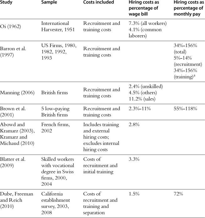
aThis is an estimate derived from Table 7.1 of Barron et al. (1997), with the reported hours of those spent on the recruiting and/or training multiplied by 1.5, a crude estimate of the relative wage of recruiters/trainers to new recruits taken from Silva and Toldeo (2009). This is then divided by an assumption of a 40 hour week to derive the fraction of a month’s pay spent on recruiting/training.
Although there is a very wide range of estimates in Table 2, some general features do emerge. First, the original Oi (1962) estimates seem in the right ballpark—with hiring costs a bit below 5% of the total labor costs. The bulk of these costs are the costs associated with training newly-hired workers and raising them to the productivity of an experienced worker. The costs of recruiting activity are much smaller. We also have evidence of heterogeneity in hiring costs, both across worker characteristics (the hiring costs of more skilled workers typically being higher) and employer characteristics (the hiring costs of large employers typically being higher). But, one should recognize that we do not know enough about the hiring process—another chapter in this volume (Oyer and Schaefer, 2011) makes a similar point.
2.1.3 Marginal and average hiring costs
It is not entirely clear from Table 2 whether we have estimates of average or marginal hiring costs—from the theoretical point of view we would like the latter more than the former. In some surveys (e.g. Barron et al., 1997) the questions on hiring costs relate to the last hire, so the responses might be interpreted as a marginal hiring cost. In other studies (e.g. Abowd and Kramarz, 2003) the question relates to all expenditure on certain activities in the past year, so are more likely to be closer to average hiring costs. In others studies, it is not clear.
To think about the relationship between average and marginal hiring costs suppose that the total cost of R recruits is given by:
![]() (3)
(3)
Then there is the following relationship between marginal hiring cost and the average hiring cost:
![]() (4)
(4)
If β is below (above) 1 there are increasing (decreasing) marginal costs of recruitment, and the marginal cost will be above (below) the average cost.
We do have some little bits of evidence on the returns to scale in hiring costs. Manning (2006), Blatter et al. (2009) and Dube, Freeman and Reich (2010) all report increasing marginal costs, although the latter study finds that only in a cross-section. However, Abowd and Kramarz (2003) and Kramarz and Michaud (2010) report decreasing marginal costs, as they estimate hiring to have a fixed cost component. However, this last result may be because they exclude the costs of recruitment, where one would expect marginal costs to be highest. The finding in Barron et al. (1997) that large firms have higher hiring costs might also be interpreted as evidence of increasing marginal costs, as large firms can only get that way by lots of hiring. Our evidence on this question is not strong, and one cannot use these studies to get a reliable point estimate of β. One can also link the question of whether there are increasing marginal costs of hiring to the older literature on employment adjustment costs (e.g. Nickell, 1986; Hamermesh, 1993)—the traditional way of modeling these adjustment costs as quadratic corresponds to increasing marginal hiring costs.
Worrying about a possible distinction between marginal and average hiring costs might seem a minor issue, but Section 4.3.4 shows why it is more important than one might have thought for how one thinks about the nature of labor markets and the likely effects of labor market regulation.
2.2 The search activity of the non-employed
2.2.1 Theory
Now consider the size of rents from the perspective of workers. One cannot use a similar methodology to that used in the previous section because, while it is reasonable to assume that vacant jobs are in potentially infinite supply, one cannot make the same assumption about unemployed workers. The approach taken here is that if employment offers sizeable rents we would expect to see the unemployed making strenuous efforts to find employment and the size of those efforts can be used as a measure of the rents.
Consider an unemployed worker who faces a wage offer distribution, F(w), and can influence the arrival rate of job offers, λ, by spending time on job search. Denote by γ the fraction of a working week spent on job search and λ(γ) the function relating the job offer arrival rate to the time spent on job search. The value of being unemployed, Vu, can then be written as:
![]() (5)
(5)
where r is the interest rate, bu is the income received when unemployed, b is the value of leisure, w* is the reservation wage (also a choice variable), and V(w) is the value of a job that pays a wage w. This is a set-up first used by Barron and Mellow (1979). Taking the first order condition for the time spent on job search, γ:
![]() (6)
(6)
This shows us that the incentive for workers to generate wage offers is related to the rents they will get from those offers. Let us rearrange (6) to give us:
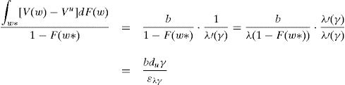 (7)
(7)
where ελγ is the elasticity of the job offer arrival rate with respect to search effort and du is the expected duration of unemployment5.
The left-hand side of (7) is the rents from employment averaged over all the jobs the unemployed worker might get. This is unobservable and what we would like to estimate. Equation (7) says that these average rents should be equated to the monetary value of leisure multiplied by the expected total time spent searching until getting a job (which is the duration of unemployment multiplied by time per week spent on job search) divided by the inverse of the elasticity of the job offer arrival rate to search effort. All of these elements are things that we might hope to be able to estimate, some more easily than others.
The intuition for (7) is simple—if workers typically get rents from jobs we would expect to see them willing to expend considerable amounts of time and money to get a job. However, to convert the right-hand side of (7) to monetary units we need a monetary value for leisure when unemployed. We would like to normalize these costs to get an estimate of the “per period” rent. Appendix A works through a very simple model to sketch how one might do that and derives the following formula for the gap between the average wage, ![]() , and the reservation wage, w*:
, and the reservation wage, w*:
![]() (8)
(8)
where ρ is the income when unemployed as a fraction of the reservation wage and u is the steady-state unemployment rate for the worker. The elements on the right-hand side of (8) are all elements we might hope to estimate.
2.2.2 Evidence
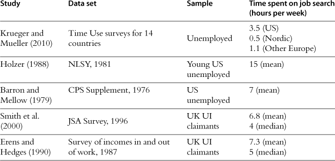
A crucial element in (8) is the fraction of a working week that the unemployed spend on job search. Table 3 provides a set of estimates of the time spent on job search by the unemployed, though such estimates are not as numerous as one would like. Probably the most striking fact about the job search activity of the unemployed is often how small is the amount of time they seem to spend on it. The most recent study is the cross-country comparison of Krueger and Mueller (2010), who use time-use surveys to conclude that the average unemployed person spends approximately 4 minutes a day on job search in the Nordic countries, 10 minutes in the rest of Europe, and 30 minutes in North America. But the other US and UK studies reported in Table 3 find higher levels of job search6. These studies use a methodology where a direct question is asked of the unemployed about the amount of time spent searching, a very different methodology from the time-use studies. However, even these studies do not suggest a huge amount of time spent unemployed as it is essentially a part-time activity. Taking these numbers at face value they perhaps suggest a value for γ in the region of 0.1–0.2.
If one assumed that the steady-state unemployment rate for currently unemployed workers is 10%, and that the replacement rate was 0 and that ελγ was 1 so that a doubling of search effort leads to a doubling of the job offer arrival rate, one would conclude from the use of the formula in (8) that the rents for unemployed workers are small, no more than 2%. However, there are a number of reasons to be cautious about this conclusion.
First, the formula in (8) is very sensitive to the assumed value of ελγ. If increases in search time lead to little improvement in job offer arrival rates, a small amount of job search is consistent with large rents. Ideally we would like to have some experimental evidence on what happens when we force individuals to increase job search activity. Although there are a large number of studies (many experimental or quasi-experimental), that seek to estimate the effect of programmes designed to assist with job search on various outcomes for the unemployment, many of these job search assistance programs combine more checking on the job search activity of the unemployed with help to make search more effective. For current purposes we would like only the former. One study that seems to come close is Klepinger et al. (2002) which investigates the effect of Maryland doubling the number of required employer contacts from 2 to 4. This doubling of required contacts significantly reduced the number of weeks of UI receipt by 0.7 weeks on a base of 11.9 so a doubling in the required number of contacts reduces unemployment durations by 6%. Assuming that the doubling of the number of contacts doubles the cost leads to a very small implied elasticity of 0.04. There are a number of reasons to be cautious—we do not have evidence about how much employer contacts were actually increased and, second, when individuals are forced to comply with increased employer contacts they would not choose for themselves, they will probably choose low-cost but ineffective contacts. These would tend to lead to lower estimates of the elasticity. On the other hand exits from UI are not the same as exits to employment and the employment outcomes are not so favorable.
There are also a number of non-experimental studies that seek to relate unemployment durations to job search intensity, with mixed results that suggest caution in interpretation. For example, Holzer (1987) reports estimates for the effect of time spent on a variety of search methods on the probability of gaining new employment (though he also controls for the number of search methods used)—many of the estimated effects are insignificant or even “wrongly-signed”.
Secondly, the formula in (8) assumes that the cost of time in job search and employment can be equated. However, the time cost of job search may be higher than one might think as Krueger and Mueller (2010) find that levels of sadness and stress are high for the unemployed while looking for a job and levels of happiness are low. If these emotional costs are high, the cost of job search will be higher than one otherwise would have thought, reducing the incentives to spend time on it.
Thirdly, while job search seems to use more time than money (something that motivated the model used here), the monetary cost is not zero. While the unemployed have a lot of time on their hands, they are short of money. Studies like Card et al. (2007) suggest that the unemployed are unable to smooth consumption across periods of employment and unemployment so that the marginal utility of income for the unemployed may be much higher than for the employed. For example, in the UK evaluation of the Job Seekers’ Allowance, one-third of UI recipients reported that their job search was limited because of the costs involved, with the specific costs most commonly mentioned being travel, stationery, postage and phone. If time and money are complements in the job search production function, low expenditure will tend to be related to low time spent.
Finally, DellaVigna and Daniele Paserman (2005) investigate the effect of hyperbolic discounting in a job search model. They present evidence that, in line with theoretical predictions, the impatient engage in lower levels of job search and have longer unemployment durations. If this is the right model of behavior one would have to up-rate the costs of job search by the degree of impatience to get an estimate of the size of rents from jobs.
So, the bottom line is that although the fact that the unemployed do not seem to expand huge amounts of effort into trying to get employment might lead one to conclude that the rents are not large, there are reasons why such a conclusion might be hasty. And we do have other evidence that the unemployed are worse off than the employed in terms of well-being—see, for example, Clark and Oswald (1994), Krueger and Mueller (2010). I would be hesitant to conclude that the rents from employment are small for the unemployed because of the low levels of search activity as I suspect that if one told a room of the unemployed that their apathy showed they did not care about having a job, one would get a fairly rough reception. When asked to explain low levels of search activity, one would be much more likely to hear the answer “there is no point”, i.e. they say that the marginal return to more search effort, ελγ, is low.
One possible explanation for why the unemployed do not spend more time on job search is that the matching process is better characterized by stock-flow matching rather than the more familiar stock-stock matching (Coles and Smith, 1998; Ebrahimy and Shimer, 2010). In stock-flow matching newly unemployed workers quickly exhaust the stock of existing vacancies in which they might be interested and then rely on the inflow of new vacancies for potential matches. It may be that rapid exhaustion of possible jobs provides a plausible reason for why, at the margin, there is little return to extra job search.
Before we move on, it is worth mentioning some studies that have direct estimates of the left-hand side of (8). These are typically studies of the unemployed that ask them about the lowest wage they would accept (their reservation wage) and the wage they expect to get. For example Lancaster and Chesher (1983) report that expected wages are 14% above reservation wages. The author’s own calculations on the British Household Panel Study, 1991–2007 suggest a mean gap of 21 log points and a median gap of 15 log points. These estimates are vulnerable to the criticism that they are subjective answers, though the answers do predict durations of unemployment and realized wages in the expected way7. They are perhaps best thought of as very rough orders of magnitude
The discussion has been phrased in terms of a search for the level of worker rents, ignoring heterogeneity. However, it should be recognized that there are a lot of people without jobs who do not spend any time looking for a job. For this group—classified in labor market statistics as the inactive—the expected rents from the employment relationship must be too small to justify job search. The fact that some without jobs search and some do not strongly suggests there is a lot of heterogeneity in the size of rents or expected rents. Once one recognizes the existence of heterogeneity one needs to worry about the population whose rents one is trying to measure. The methodology here might be useful to tell us about the rents for the unemployed but we would probably expect that the average rents for the unemployed are lower than for the employed. Estimating the rents for the employed is the subject of the next section.
2.3 The costs of job loss
To estimate rents for the employed, the experiment one would like to run is to consider what happens when workers are randomly separated from jobs. There is a literature that considers exactly that question—studies of displaced workers (Jacobson et al., 1993; Von Wachter, Manchester and Song, 2009). One concern is the difficulty of finding good control groups, e.g. the reason for displacement is presumably employer surplus falling to less than zero. But, for some not totally explained reason, it seems that wages prior to displacement are not very different for treatment and control groups—it is only post-displacement that one sees the big differences. Under this assumption one can equate these estimates to loss of worker surplus.
For a sample of men with 5 years previous employment who lost their jobs in mass lay-offs in 1982, Von Wachter, Manchester and Song (2009) estimate initial earnings losses of 33% that then fall but remain close to 20% after 20 years. Similar estimates are reported in Von Wachter, Bender and Schmeider (2009) for Germany. These samples are workers who might plausibly be expected to have accumulated significant amounts of specific human capital, so one would not be surprised to find large estimated rents for this group. However, Von Wachter, Manchester and Song (2009) find sizeable though smaller earnings losses for men with less stable employment histories pre-displacement and for women. At the other extreme, Von Wachter and Bender (2006) examine the effects of displacement on young apprentices in Germany. For this group, where we would expect rents to be small, they find an initial earnings loss of 10%, but this is reduced to zero after 5 years.
We also have a number of other studies looking at how the nature of displacement affects the size of earnings losses. Neal (1995), and Poletaev and Robinson (2008) show that workers who do not change industry or occupation or whose post-displacement job uses a similar mix of skills have much smaller earnings losses. This is as one would expect given what was said earlier about the reason for rents being the lack of an alternative employer who is a perfect substitute for the present one. Those displaced workers fortunate enough to find another job which is a close substitute for the one lost would be expected to have little or no earnings loss. But, the sizeable group of workers whose post-displacement job is not a perfect substitute for the one lost will suffer larger earnings losses. For example, Poletaev and Robinson (2008) estimated an average cost of displacement for all workers of 7% but the 25% of workers who switch to a job with a very different skill portfolio suffer losses of 15%. The fact that 25% of workers cannot find a new job that is a close match to their previous one suggests there are not a large number of employers offering jobs that are perfect substitutes for each other.
2.4 Conclusions
The methods discussed in this section can be used to give us ballpark estimates of the extent of imperfect competition in labor markets. They perhaps suggest total rents in the 15–30% range with, perhaps, most of the rents being on the worker side. However, one should acknowledge there is a lot of variation in rents and enormous uncertainty in these calculations. Because we have discussed estimates of the rents accruing to employers and workers, one might also think about using these estimates to give us some idea of how the rents are split between worker and employer. However, because none of the estimates come from the same employment relationship, that would be an unwise thing to do. The next section discusses models of the balance of power between employers and workers and these are reviewed in the next section.
3 Models of wage determination
When there are rents in the employment relationship, one has to model how these rents are split between worker and employer, i.e. one needs a model of wage determination. This is a very old problem in economics in general and labor economics in particular, going back to the discussion of Edgeworth (1932), where he argued that the terms of exchange in a bilateral monopoly were indeterminate. That problem has never been definitively resolved, and that is probably because it cannot be. In this section we describe the two main approaches found in the literature and compare and contrast them.
3.1 Bargaining and posting
The two main approaches that have been taken to modeling wage determination in recent years are what we will call ex post wage-bargaining and ex ante wage-posting (though we briefly discuss others at the end of the section). In ex post wage-bargaining the wage is split after the worker and employer have been matched, according to some sharing rule, most commonly an asymmetric Nash bargain. In ex ante wage-posting the wage is set unilaterally by the employer before the worker and employer meet.
These two traditions have been used in very different ways. The bargaining models are the preferred models in macroeconomic applications (see Rogerson and Shimer, 2011) while microeconomic applications tend to use wage-posting8. But, what is often not very clear to students entering this area is why these differences in tradition have emerged and what are the consequences. Are these differences based on good reasons, bad reasons or no reasons at all? Here we try to provide an overview which, while simplistic, captures the most important differences.
Although the models used are almost always dynamic, the ideas can be captured in a very simple static model and that is what we do here. The simple static model derives from Hall and Lazear (1984) who discuss a wider set of wage-setting mechanisms than we do here. Assume that there are firms, which differ in their marginal productivity of labor, p. A firm is assumed to be able to employ only one worker.
In ex post wage-bargaining models, the wage in a match between a worker with leisure value b and a firm with productivity p is chosen to maximize an asymmetric Nash bargain:
![]() (9)
(9)
leading to a wage equation:
![]() (10)
(10)
where α can be thought of as the bargaining power of the worker, which is typically thought of as exogenous to the model. The match will be consummated whenever there is some surplus to be shared, i.e. whenever p ≥ b so that there is ex post efficiency. There will not necessarily be ex ante efficiency if worker or employer or both have to make investments ahead of a match, investments either in the probability of getting a match or in the size of rents when a match is made. For example, if α = 0 workers get no surplus from the employment relationship so would not invest any time in trying to find a job.
Now consider a wage-posting model in which employers set the wage before being matched with a worker. To derive the optimal wage in this case we need to make some assumption about the process by which workers and employers are matched—for the moment, assume that is random though alternatives are discussed below. And assume that workers differ in their value of leisure, b—denote the distribution function of this across workers by G(b).
If the firm sets a wage w, a worker will accept the offer if w > b, something that happens with probability G(w). So expected profits will be given by:
![]() (11)
(11)
This leads to the following first-order condition for wages:
![]() (12)
(12)
where ε is the elasticity of the function G with respect to its argument and the notation used reflects the fact that this elasticity will typically be endogenous. Higher productivity firms offer higher wages. An important distinction from ex post wage-bargaining is that not all ex post surplus is exploited—some matches with positive surplus (i.e. with p > b) may not be consummated because b > w. In matches that are consummated the rents are split between employers and workers, so employers are unable to extract all surplus from workers even though employers can unilaterally set wages.
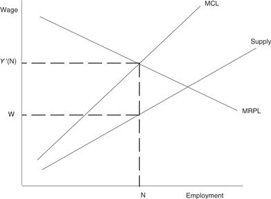
In this model G(w) can be thought of as the labor supply curve facing the firm, in which case can think of it as a standard model of monopsony in which the labor supply to a firm is not perfectly elastic and (12) as the standard formula for the optimal wage of a monopsonist. There is a simple and familiar graphical representation of the decision-making problem for the firm—see Fig. 1. In contrast, there is no such simple representation for the outcome of the ex post wage-bargaining model9.
One might think that the two wage Eqs (10) and (12) are very different. But they can easily be made to look more similar. Suppose that the supply of labor can be written as:
![]() (13)
(13)
where b0 is now to be interpreted, not as a specific worker’s reservation wage, but as the lowest wage any worker will work for. Then the wage equation in (11) can be written as:
![]() (14)
(14)
which is isomorphic to (9) with ![]() . In some sense, the bargaining power of workers in the wage-posting model is measured by the elasticity of the labor supply curve to the firm. However, note that the interpretation of the reservation wage in (10) and (14) is different—in (10) it is the individual worker’s reservation wage while in (14) it is the general level of reservation wages measured by the lowest in the market.
. In some sense, the bargaining power of workers in the wage-posting model is measured by the elasticity of the labor supply curve to the firm. However, note that the interpretation of the reservation wage in (10) and (14) is different—in (10) it is the individual worker’s reservation wage while in (14) it is the general level of reservation wages measured by the lowest in the market.
The assumption of random matching plays an important role in the nature of the wage-posting equilibrium so it is instructive to consider other models of the matching process. The main alternative to random matching is “directed search” (see, for example, Moen, 1997). Models of directed search typically assume that there is wage-posting but that all wage offers can be observed before workers decide on their applications.
Although models of directed search make the same assumption about the availability of information on wage offers as models of perfect competition (i.e. complete information), they do not assume that an application necessarily leads to a job, so there is typically some frictional unemployment in equilibrium caused by a coordination problem. So the expected utility of a worker applying to a particular firm is not just the wage, but needs to take account of the probability of getting a job. In the simplest model this expected utility must be equalized across jobs, giving the model a quasi-competitive feel, and it is perhaps then no surprise that the outcomes are efficient. The literature has evolved with different assumptions being made about the number of applications that can be made, what happens if workers get more than one job offer, what happens if the first worker offered a job does not want it (e.g. Albrecht et al., 2006; Galenianos and Kircher, 2009; Kircher, 2009). It would be helpful to have some general principles which help us understand the exact feature of these models that do and do not deliver efficiency.
3.2 The right model?
Rogerson et al. (2005, p. 984) conclude their survey of search models by writing that one of the unanswered questions is “what is the right model of wages?”, with the two models described above being the main contenders. If we wanted to choose between these two descriptions of the wage determination process, how would we do so? We might think about using theoretical or empirical arguments. As economists abhor unexploited surpluses, theory would seem to favor the ex post wage-bargaining models in which no match with positive surplus ever fails to be consummated10. One might expect that there would be renegotiation of the wage in a wage-posting model if p > b > w.
However, over a very long period of time, many economists have felt that this account is over-simplistic, that wages, for reasons that are not entirely understood, have some form of rigidity in them that prevents all surplus being extracted from the employment relationship. There are a number of possible reasons suggested for this. Hall and Lazear (1984) argue this is caused by informational imperfections while Ellingsen and Rosen (2003) argue that wage-posting represents a credible commitment not to negotiate wages with workers something that would cost resources and raise wages. There is also the feeling that workers care greatly about notions of fairness (e.g. see Mas, 2006) so that this makes it costly to vary wages for workers who see themselves as equals. There is also the point that if jobs were only ever destroyed when there was no surplus left to either side, there would be no useful distinction between quits and lay-offs, though most labor economists do think that distinction meaningful and workers losing their jobs are generally unhappy about it. The bottom line is that theory alone does not seem to resolve the argument about the “best” model of wage determination.
What about empirical evidence? In a recent paper Hall and Krueger (2008) use a survey to investigate the extent to which newly-hired workers felt the wage was a “take-it-or-leave-it” offer, as ex ante wage-posting models would suggest. All those who felt there was some scope for negotiation are regarded as being ex post wage-bargaining. They show that both institutions are common in the labor market, with negotiation being more prevalent. In low-skill labor markets wage-posting is more common than in high-skill labor markets, as perhaps intuition would suggest.
This direct attempt to get to the heart of the issue is interesting, informative and novel, but the classification is not without its problems. For example, some of those who report a non-negotiable wage may never have discovered that they had more ability to negotiate over the wage than the employer (successfully) gave them the impression there was. For example, Babcock and Laschever (2003) argue that women are less likely to negotiate wages than men and more likely to simply accept the first wage they are offered.
Similarly, there are potential problems with assuming that all those without stated ex ante wages represent cases of bargaining. For example, employers with all the bargaining power would like to act as a discriminating monopsonist tailoring their wage offer to the circumstances of the individual worker, not the simple monopsonist the wage-posting model assumes. Hall and Krueger (2008) are aware of this line of argument but argue it is not relevant because wage discrimination would result in all workers in the US being held to their reservation wage, a patently ridiculous claim. But, there is a big leap from saying some monopsonistic discrimination is practiced to saying it is done perfectly, so this argument is not completely compelling.
There is also the problem that the methodology used, while undoubtedly fascinating and insightful, primarily counts types of contract without looking at the economic consequences. For example, Lewis (1989, p. 149) describes how Salomon Brothers lost their most profitable bond-trader because of their refusal to break a company policy capping the salary they would pay. Undoubtedly, this contract should be described as individualistic wage-bargaining, but there were limits placed on that which resulted in some ex post surplus being lost as suggested by the wage-posting models.
One possible way of resolving these issues would be to look at outcomes. For example, ex post individualistic wage-bargaining would suggest, as from (10), that there would be considerable variation in wages within firms between workers with different reservation wages—see (10). On the other hand, ex ante wage-posting would suggest no wage variation within firms between workers with different reservation wages. Machin and Manning (2004) examine the structure of wages in a low-skill labor market, that of care workers in retirement homes. They find that, compared to all other characteristics of the workers, a much greater share of the total wage variation is between as opposed to within firms. Reservation wages are not observed directly, but we might expect to be correlated with those characteristics, so ex post wage-bargaining would predict correlations of wages with those variables11.
One could spend an enormous amount of time debating the “right” model of wage determination. But we will probably never be able to resolve it because the labor market is very heterogeneous, so that no one single model fits all, so the question of “what is the right model?” is ill-posed. In fact, it is the very existence of rents that gives the breathing-space in the determination of wages in which the observed multiplicity of institutions can survive. In a perfectly competitive market an employer would have no choice but to pay the market wage and to deviate from that, even slightly, leads to disaster.
It is also worth reflecting that, in many regards, wage-bargaining and wage-posting models are quite similar (e.g. they both imply that rents are split between worker and employer) so that it may not make very much difference which model one uses as a modeling device. The main substantive issue in which they differ is in whether one thinks that all ex post surplus is extracted. But, because even ex post efficiency does not mean ex ante efficiency, this may not be such a big difference in practice. However, this is not to say that the choice of model has had no consequences for labor economics because too many economists see the labor market only through the prism of the labor market model with which they are most familiar.
For example, as illustrated above, a wage-posting model naturally leads one to think in terms of the elasticity of the labor supply curve to an individual firm and that one can represent the wage decision using the familiar diagram of Fig. 1. It is easy to forge links with other parts of labor economics, so it is perhaps not surprising that this has often been the model of choice for microeconomic models of imperfect competition in the labor market. It is much more difficult to forge such links with an ex post bargaining model and the literature that uses such models sometimes seems to have developed in a parallel universe to more conventional labor economics and has concentrated on macroeconomic applications.
3.3 Other perspectives on wage determination
I have described the two most commonly found models of wage determination. But just as I have emphasized that one should not be thought as obviously “better” than the other, so one should not assume that these are the only possibles. Here we simply review some of the others that can be found in the literature. We make no attempt to be exhaustive (e.g. see Hall and Lazear, 1984, for a discussion of a range of possibilities we do not discuss here).
The simple model sketched above only has workers moving into jobs from non-employment because it is a one-period model. In reality, over half of new recruits are from other jobs (Manning, 2003a; Nagypal, 2005) so that one has to think about how wages are determined when a worker has a choice between two employers.
In models with ex-post wage-bargaining, on-the-job search is a bit tricky to incorporate into standard models because it is not clear how to model the outcome of bargaining when workers have a choice of more than one employer, and different papers have taken different approaches, e.g. Pissarides (1994) assumes that the fall-back position for workers with two potential employers is unemployment while Cahuc et al. (2006) propose that the marginal product at the lower productivity firm be the outside option. Shimer (2006) points out that the value function for employed workers is typically convex in the wage when there is the possibility of moving to a higher-wage job in the future, and derives another bargaining solution, albeit one with many equilibria.
In contrast, models based on wage-posting do not find it hard to incorporate on-the-job search, as they typically simply assume that the worker accepts the higher of the two wage offers. But, they do find it difficult to explain why the employer about to lose a worker does not seek to retain them by raising wages. A number of papers look at the institution of offer-matching (Postel-Vinay and Robin, 2002) in which the two employers engage in Bertrand competition for the worker. However, many have felt that offer-matching is not very pervasive in labor markets and have offered reasons for why this might be the case (see, for example, the discussion in Hall and Lazear, 1984).
4 Estimates of rent-splitting
The previous section reviewed theoretical models of the ways in which rents are divided between workers and employers—this section reviews empirical evidence on the same subject.
Section 2 reviewed some ways in which one might get some idea of the size of rents accruing to employers and workers. Because it produced estimates of the rents accruing to employer and worker, one could use these estimates to get some idea of how the rents are shared between employer and worker. But, because these estimates are assembled from a few, disparate sources of evidence, we have no study in which we could estimate both employer and worker rents in the same labor market, so that estimating how rents are shared by using an estimate of employer rents in one labor market and worker rents in another would not deliver credible evidence. So, in this section we review some other methodologies that can be thought of as seeking to estimate the way in which rents are split between worker and employer.
The part of the literature on imperfect competition in labor markets that has used ex post wage-bargaining as the model of wage determination and, consequently, uses an equation like (10) would tend to see rents being split according to the bargaining power of the workers. The studies that attempt to estimate a rent-sharing parameter are reviewed in Section 4.1. In contrast, models that are based on wage-posting have a monopsony perspective on the labor market and view the elasticity of the labor supply curve facing the employer as the key determinant of how rents are split. We review these ideas in Sections 4.2 and 4.3. Finally, we briefly review some studies that have sought to use estimates of the extent of frictions in the labor market to estimate how rents are divided.
4.1 Estimates of rent-sharing
In a bargaining framework, we are interested in how wages respond to changes in the surplus in the employment relationship, i.e. to measure something like (10). There is a small empirical literature that seeks to estimate the responsiveness of wages to measures of rents. These studies differ in the theoretical foundation for the estimated equation, the way in which the rent-sharing equation is measured and the empirical methodology used.
The Eq. (10) was derived from a model of bargaining between a worker and employer where the bargaining relationship covers only one worker. But, there are alternative ways of deriving a similar equation from other models. For example, Abowd and Lemieux (1993) assume that the firm consists of a potentially variable number of workers with a revenue function F(N), and that the firm bargains with a union with preferences N(w – b) over both wages and employment, i.e. we have an efficient bargaining model (McDonald and Solow, 1981). That is, wages and employment are chosen to maximize:
![]() (15)
(15)
One way of writing the first-order condition for wages in this maximization problem is:
![]() (16)
(16)
i.e. wages are a weighted average of revenue per worker and reservation wages with the weight on revenue per worker being α. The similarities between (16) and (10) should be apparent as F(N)/N is the average productivity of labor. In this model employment will be set so that:
![]() (17)
(17)
There are other models from which one can derive a similar-looking equation to (16), though we will not go into details here. For example, if one assumes that employment is chosen by the employer given the negotiated wage (what is sometimes called the right-to-manage or labor demand curve model—see, for example, Booth, 1995) or a more general set of ”union” preferences.
In all the specifications derived so far, it is a measure of revenue per worker or quasirents per worker put on the right-hand side. But, many studies write the wage equation in terms of profits per worker, i.e. take −αw from both sides of (16) and write it as:
![]() (18)
(18)
In all these cases it should be apparent that the outcome of rent per worker or profit per worker is potentially endogenous to wages, so that OLS estimation of these equations is likely to lead to biased estimates. Hence, some instrument is used, and the obvious instrument is something that affects the revenue function for the individual firm but does not affect the wider labor market (here measured by b). Although revenue function shifters sound very plausible, it is not clear that they are good instruments. For example if the revenue function is Cobb-Douglas (so the elasticity of revenue with respect to employment is a constant) then the marginal revenue product of labor is proportional to the average revenue product and the employment equation in (17) makes clear the marginal revenue product will not be affected by variables that affect the revenue function. In this case shifts in the revenue function result in rises in employment such that rents per worker and wages are unchanged12. The discussion in Abowd and Lemieux (1993, p. 987) is very good on this point. In cases close to this, instruments based on revenue function shifters will be weak. Many of the rent-sharing studies are from before the period when researchers were aware of the weak instrument problem (see Angrist and Pischke, 2008, for a discussion) and the instruments in some studies (e.g. Abowd and Lemieux, 1993) do not appear to be strong.
Some estimates of the rent-sharing parameter are shown in Table 4. In this table we have restricted attention to those that estimate an equation that is either in the form of (16) or (18) or can be readily transformed to it13. Table 4 briefly summarizes the data used in each study, the measure of rents or profits used, and the method (if any) used to deal with the endogeneity problem. In some studies the instruments are lags of various variables while others use exogenous shifts to demand, e.g. as caused by exchange rate movements. There are a couple of “case studies” of the impact of de-regulation in various industries.
Table 4
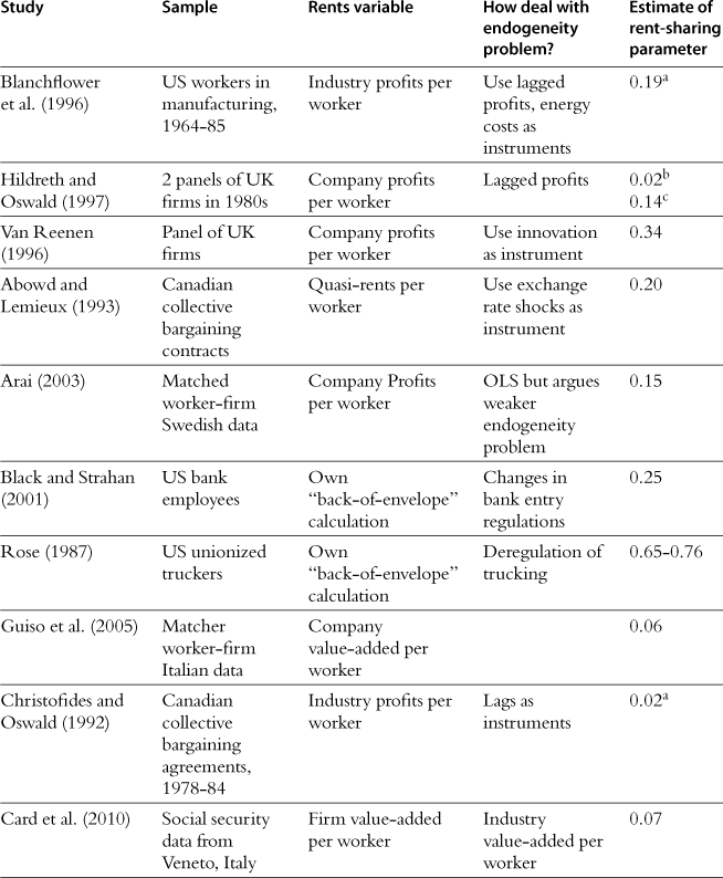
aThe equation is estimated with log earnings as dependent variable and rent-sharing parameter derived using reported figures for average profits per worker and a labor share in value-added of 75%.
bThis is computed using ratio of reported levels of earnings to profits per head in the data which is extremely low at 1.1. Using a ratio of 2 or 3 would raise these estimates considerably.
cThis is computed using ratio of reported levels of earnings to profits per head in the data which is high at 5.3. Using a ratio of 2 or 3 would lower these estimates considerably.
What one would ideally like to measure is the effect of a change in rents in a single firm on wages in that firm. It is not clear whether that is what is being estimated. For example, several studies in Table 4 use industry profits as a measure of rents. If labor has any industry-specific aspect to it then a positive shock to industry profits would be expected to raise the demand for labor in a competitive market and, hence, raise the general level of wages (represented by b in the model above)14. If this is important one would expect that the estimates reported in Table 4 are biased upwards. And the studies that use firm-level profits or rents but instrument by industry demand shifters are potentially vulnerable to the same criticism.
The final column in Table 4 presents estimates of the α implied by the estimates. Most of these studies do not report an estimate of α directly (e.g. the dependent variable is normally in logs whereas the theoretical idea is in levels) so a conversion has taken place based on other information provided or approximations. For example if the equation is specified with the log of wages on the left-hand side and the log of profits on the right-hand side so that the reported coefficient is an elasticity then one needs to multiply by the ratio of wages to profits per head to get the implied estimate of α. If, for example the share of labor in value-added is 75% then one needs to multiply the coefficient by 3, while if it is 66% one needs to multiply by 2. In addition there is a wide variation in the reported ratio of wages to profit per head in the data sets used in the studies summarized in Table 4 from a minimum of 1.1 to a maximum of 5.3. Unsurprisingly this can make a very large difference to the estimates of α and this is reflected in Table 4. In addition, the difficulty in computing the “true” measure of profits or rents may also lead to considerable variation in estimates.
There are a number of studies (Christofides and Oswald, 1992; one of the samples in Hildreth and Oswald, 1997) where α is estimate to be close to zero, but a number of other estimates are in the region 0.2-0.25. Studies from Continental European countries—the Italian and Swedish studies of Arai (2003), Guiso et al. (2005) and Card et al. (2010)— are markedly lower—this might be explained by the wage-setting institutions in those countries where one might expect the influence of firm-level factors to be less important than in the US (see the neglected Teulings and Hartog, 1998, for further elaboration of this point) though there are also some methodological differences from the other studies. And the study of Rose (1987) also looks an outlier with an estimate of α around 0.7. However, this estimate is derived using some back-of-the-envelope calculations and is for a very specific industry so may not be representative. It is worth remarking that all of these studies suggest that most rents accrue to employers, not workers while the direct estimates of the size of rents accruing to employer and workers in previous sections perhaps suggested the opposite. That is an issue that needs to be resolved.
The estimates of α discussed so far have all been derived from microeconomic studies. But the rent-splitting parameter also plays an important role in macroeconomic models of the labor market, and such studies often use a particular value. It has been common to assume the rent-splitting parameter is set to satisfy the Hosios condition for efficiency (often around 0.4), though no convincing reason for that is given, sometimes calibrated or estimated to help to explain some aspects of labor market data (and Hagedorn and Manovskii, 2008 suggest a value of 0.05 based on some of the studies reported in Table 4). A recent development (e.g. Pissarides, 2009; Elsby and Michaels, 2008) has been to argue that there is an important difference between the sensitivity of the wages of new hires and continuing workers to labor market conditions. The micro studies reviewed in Table 4 have not pursued this dimension.
Many of the studies summarized in Table 4 are of unionized firms, motivated by the idea that non-union firms are much less likely to have rent-sharing. Although a perspective that there are pervasive rents in the labor market would lead one to expect that even non-union workers get a share of the rents, one might expect unions to be institutions better-able to extract rents for workers, so that one would estimate a higher α in the union sector. But the few studies that distinguish between union and non-union sectors (e.g. Blanchflower et al., 1996, 199015) often find that, if anything, the estimate of α is larger in the non-union sector. However, this is what one might expect from a wageposting perspective, because a union setting a take-it-or-leave-it wage makes the labor supply to a firm more wage elastic (like the minimum wage) than that faced by a nonunion firm. Hence, one then predicts one would find a higher rent-sharing parameter in the non-union sector. This leads on to estimates of rent-sharing based on the elasticity of the labor supply curve to employers.
4.2 The elasticity of the labor supply curve to an individual employer
As the formula in (12) makes clear, a wage-posting model would suggest that it is the elasticity of the labor supply curve facing the employer that determines how rents are split between worker and employer. This section reviews estimates of that elasticity. An ideal experiment that one would like to run to estimate the elasticity of the labor supply curve to a single firm would be to randomly vary the wage paid by the single firm and observe what happens to employment. As yet, the literature does not have a study of such an experiment.
What we do have are a number of quasi-experiments where there have been wage rises in some firms—these are summarized in Table 5. Typically those experiments have been of public sector firms where there have been perceived to be labor shortages because wages have been set below prevailing market levels. So, they sound like the type of situation where one would expect to be tracing out the elasticity of a labor supply curve.
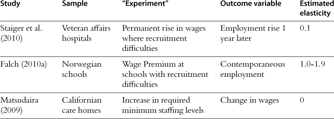
Staiger et al. (2010) examine the impact of a legislated rise in the wages paid at Veteran Affairs hospitals. They estimate the short-run elasticity in the labor supply to the firm to be very low (around 0.1), implying an enormous amount of monopsony power possessed by hospitals over their nurses. Falch (2010a) investigates the impact on the supply of teachers to individual schools in northern Norway in response to a policy experiment that selectively raised wages in some schools with past recruitment difficulties. He reports an elasticity in the supply of labor to individual firms in the region 1.0-1.9—higher than the Staiger et al study, but still very low.
Looking at these studies, one clearly comes away with the impression not that it is hard to find evidence of monopsony power but that the estimates are so enormous to be an embarrassment even for those who believe this is the right approach to labor markets. The wage elasticities are too large to be credible.
This means it makes sense to reflect on possible biases. There are a number of possibilities that come to mind. First, some of these studies only look at the response of employment to wage changes over a relatively small time horizon. As one would expect supply elasticities to be smaller in the short-run, these estimates are not reliable as estimates of the long-run elasticity. There is a simple back-of-the-envelope rule that can be used to link short-run and long-run elasticities. Boal and Ransom (1997) and Manning (2003a, chapter 2) show that if the following simple model is used for the supply of labor to a firm:
![]() (19)
(19)
where s(w) is the separation rate and R(w) is the recruitment rate, then there is the following relationship between the short-run and long-run elasticities:
![]() (20)
(20)
So one needs to divide the short-run elasticity by the quit rate to get an estimate of the long-run elasticity. If, for example, labor turnover rates are about 20% then one needs to multiply the estimates of short-run elasticities by 5 to get a better estimate of the long-run elasticity.
A second issue is whether the wage premia are expected to be temporary or permanent. If they are only temporary then one would not expect to see such a large supply response. In this regard, it is reasonable to think of the wage increases studied by Staiger et al. (2010) as permanent, those studied by Falch (2010a) as temporary. It is not clear whether an argument that the wage premia were viewed as only temporary are plausible as explanations of the low labor supply elasticities found.
Here, I suggest that there is another, as yet unrecognized, problem with these estimates of labor supply elasticities. The reason for believing this comes from thinking about estimates of the labor supply elasticities from an alternative experiment—force an employer to raise its employment level and watch what happens to the wages that they pay. This is what is analyzed by Matsudaira (2009) who analyzes the effect of a 1999 California law that required all licensed nursing homes to maintain a minimum number of hours of nurses per patient. This can be thought of as a mandated increase in the level of employment.
According the simplest models of monopsony in which there is a one-to-one relationship between wages and labor supply to the firm, the wage response to the mandated employment increase should give us an estimate of the inverse of the wage elasticity. If the studies of mandated wage increases cited above are correct and the labor supply elasticity is very small, we should see very large wage increases in response to mandated employment changes. This is especially true if the short-run elasticity is very low. In fact, Matsudaira finds that firms that were particularly affected by the mandated increased in employment did not raise their wages relative to other firms who were not affected. As a result, the labor supply to the employer appears very elastic, seemingly inconsistent with studies of mandated wage increases. It is possible that, as these are studies of different labor markets there is no apparent inconsistency but I would suggest that is not the most likely explanation and that the real explanation is a problem with the simple model of monopsony.
How can we reconcile these apparently conflicting findings? The problem with the simple-minded model of monopsony is that it assumes that the only way an employer can raise employment is by raising its wage. A moment’s reflection should persuade us that this is not very plausible. There are a number of possible reasons for this—I will concentrate on one in some detail and then mention others.
We have already seen that hiring costs money and used estimates of these hiring costs to shed light on the size of employer rents from the employment relationship. If employers want to hire more workers, they can spend more resources on trying to recruit workers, e.g. advertising vacancies more frequently or extensively. Hence, the supply of workers to the firm will then be a function not just of the wage but also of the expenditure on recruitment. This model is examined in Manning (2006), who terms it the “generalized model of monopsony” and it can easily explain the paradox described above.
To see how it can do this assume there are constant marginal hiring costs, h(w), which might depend on the wage. If the separation rate is s(w) a flow of s(w)N recruits is necessary for the employer to maintain employment at N which will cost s(w)h(w)N. This represents the per period expenditure on recruitment necessary to keep employment at N if the wage paid is w. Note that, unlike the simple monopsony model, any level of employment is compatible with any level of the wage but that there are associated recruitment costs. If, in the interests of simplicity, we ignore discounting (the recruitment costs of a worker must be paid up-front but profits accrue in the future), the profits of the firm can be written as:
![]() (21)
(21)
First, consider the choices of wage and employment by an unconstrained profit-maximizing firm. The wage will be chosen to satisfy the first-order condition:
![]() (22)
(22)
Denote this choice by w*. The first-order condition for employment will then be:
![]() (23)
(23)
Now, consider what happens in this model when we mandate wages or mandate employment. Consider, mandated employment first, as in the Matsudaira paper. If the government requires an increase in employment, the optimal thing for the firm to do is to increase recruitment activity—the optimal wage (22) remains completely unchanged. This is, to a first approximation, what Matsudaira finds. However, it tells us nothing about the degree of imperfect competition in the labor market which is related to the elasticity of separation rates and recruitment with respect to the wage.
Now consider a mandated increase in the wage. This reduces separations and may reduce the marginal cost of recruitment. But, if it is a small increase from the optimal wage the first-order effect will be to leave employment unchanged—the employer responds by reducing recruitment expenditure. One might explain the small positive effects on employment found in the literature as being the result of mandated wage increases in public sector firms where wages had been held artificially low.
In the generalized model of monopsony, the two experiments of mandated wage or employment increases are no longer mirror images of each other. A rise in mandated wages which, ceteris paribus, leads to a rise in labor supply to the firm could be met with an off-setting fall in recruitment activity, leaving overall employment unchanged. On the other hand, a rise in mandated employment may be met with a rise in recruitment activity to generate the extra supply with no increase in wages. This can be understood with Fig. 2. Starting from an initial position the line labelled “mandated wage” rise tells us how employment will change if the firm is forced to raise wages. This suggests a low elasticity of supply. The line labelled “mandated employment” rise tells us how wages will change when the firm is forced to raise employment—this suggests a high elasticity of labor supply.
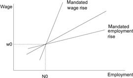
We have used a very simple model to break the one-to-one link between wages and employment found in the standard model of monopsony. The change is plausible but does substantially affect how one interprets the empirical results of estimates of the effects of raising wages on employment (or vice versa). This is not the only way in which one might seek to reconcile these conflicting empirical findings. Another alternative is to assume that workers are heterogeneous in terms of quality so that employers also face an intensive margin in deciding the cut-off quality level for workers. Employers do not simply accept all workers who apply—they reject those they deem of poor quality, and how poor one has to be to be rejected is clearly endogenous. An example in Appendix B shows how, if the distribution of worker ability in the applicant pool is exponential then firms respond to mandated wage increases by increasing worker quality and not employment, and to mandated employment increases by reducing worker quality and not increasing wages. It also shows how a model with non-wage aspects of work can deliver the same conclusion.
All of these quasi-experimental studies described above are studies of mandated changes to wages or employment which might be thought to force employers to move along their labor supply curves. But, another empirical strategy is to consider changes in variables which induce moves along the labor supply curve. To identify the labor supply curve (which is all we want here) a variable that shifts the MRPL curve without shifting the supply curve is needed. One can then use this as an instrument for the wage or employment (depending on which way round we are estimating the supply curve) in estimating the supply curve. But, of course, it requires us to be able to provide such an instrument.
If one is interested in estimating the elasticity of labor supply to an individual firm then the instrument needs to be something that affects the demand curve for that firm but has negligible impact on the labor market as a whole. The reason is that a pervasive labor market demand shock will raise the general level of wages, so is likely to affect the labor supply to an individual firm. So, for example, the approach of using demand shocks caused by exchange rate fluctuations (as in Abowd and Lemieux, 1993) does not seem viable here. Sullivan (1989) uses the population in the area surrounding the hospital as an instrument affecting the demand for nurses This is a serious attempt to deal with a difficult problem, but their instruments are not beyond criticism. If the main variation in the number of children or the number of patients comes from variation in population it is also likely that the supply of nurses in an area is proportional to population as well.
The studies reviewed in this section do provide us with the best estimates we have of how employers respond to mandated wage and employment changes. But, as has been made clear, they probably do not tell us about the wage elasticity of the labor supply to an individual firm, which was the original motivation. How we might estimate that elasticity is the subject of the next section.
4.3 The sensitivity of separations to wages
This section reviews estimates of the sensitivity of separations to wages. Although this might be thought a topic of interest in its own right, we include it here because such studies might shed some light on the elasticity of the labor supply curve to individual employers. Why this might be thought useful can be explained very simply. Suppose that the flow of recruits to a firm is R(w), that this dependent only on the wage (an assumption we relax below where we allow for recruits to also be affected by recruitment expenditure) and the separation rate is s(w) also dependent on the wage. In a steady-state, recruits must equal separations, which leads to:
![]() (24)
(24)
As pointed out by Card and Krueger (1995), this implies that:
![]() (25)
(25)
so that knowledge of the elasticities of recruitment and quits with respect to the wage can be used to estimate the elasticity of labor supply facing the firm. The elasticity of separations with respect to the wage is important here but so is the elasticity of recruits with respect to the wage. However, as discussed below there are arguments for linking the two. But, before discussing that argument, let us discuss estimates of the sensitivity of separations with respect to the wage.
There is a long tradition of being interested in the sensitivity of labor turnover to the wage, quite apart from any insight these studies might have for the extent of imperfect competition in the labor market. These studies are not confined to economics, e.g. see Griffeth et al. (2000) for a meta-analysis from the management literature. The bottom line is that, as predicted by models of imperfect competition, a robust negative correlation between the wages paid and labor turnover is generally found, so that the vast majority (though not all) of the studies reported below do find a significant link between separations and wages.
4.3.1 Experimental and quasi-experimental evidence
First, let us consider evidence on the sensitivity of separations to wages that are derived from studies where the variation in wages can be argued to be “exogenous”. These estimates are summarized in Table 6.
Table 6
Quasi-experimental estimates of wage elasticity of separation.
n.s. denotes “not significant”.
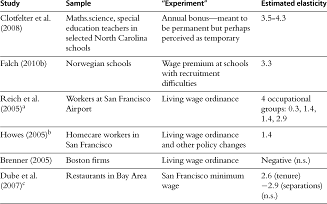
aThe estimates of the responsiveness of turnover rates to wage changes come from Table 9. Note, that there is no “control” group in Table 9.
bComputed from Table 4 in text for non-family worker. Identification is from changes in earnings over time.
cReported elasticities are derived from “full sample” estimates. Tenure and separations move in opposite directions.
Two studies, Clotfelter et al. (2008) and Falch (2010b) consider the impact on separations of policies designed to retain teachers in particular schools. The other studies reported in Table 6 analyze the effect of “living wage” ordinances (which are effectively higher minimum wages for public-sector workers or those who work for public-sector contractors), or local minimum wages. In many of these studies, separations are not the primary focus of interest and outcomes related to separations are often reported in the “other outcomes” Table.
One feature of Table 6 is the wide range of variation in the reported elasticities. Both Clotfelter et al. (2008) and Falch (2010b) report high values of the wage elasticity of separations—in the region of 3–4. A study of the wage rises at San Francisco airport (Reich et al., 2005) report a similar elasticity for one occupational group but two of the others are at 1.4 and one is at 0.25. Furthermore, Brenner (2005) reports an insignificant “wrongly-signed” elasticity, as do Dube et al. (2007) for separations—though they report a large “correctly-signed” elasticity for job tenure. Howes (2005) reports an elasticity of 1.4.
These differences may reflect the fact that the samples are very different and that there is a lot of heterogeneity across labor markets in the sensitivity of separations to the wage. But, it may also reflect the fact that these different “quasi-experiments” are estimating different elasticities. One would ideally like to see the responsiveness of separations to a permanent change in wages in a single firm holding the wages in all neighboring firms constant. It is not clear whether any of these studies does exactly that. For example, living and minimum wage changes affect the wages paid by potentially large numbers of employers in a labor market, so even if there is the control group of a labor market unaffected by the wage change one may be estimating the elasticity of separations at the level of a market as a whole to changes in wages.
4.3.2 Non-experimental studies
In this section we review non-experimental estimates of the elasticity of separations with respect to wages. In these studies the wage variable used is simply what is available. A wide range of studies is reported in Table 7.
Table 7
Non-experimental estimates of wage elasticity of separation.
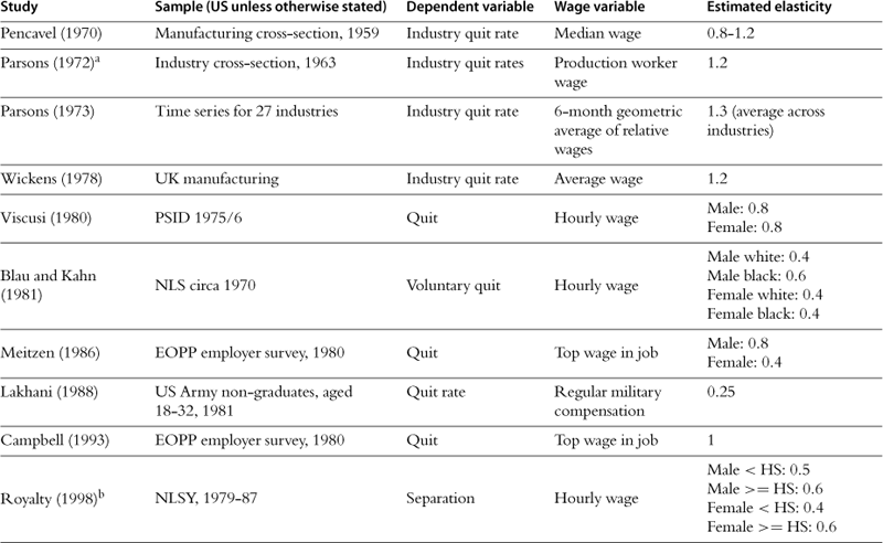
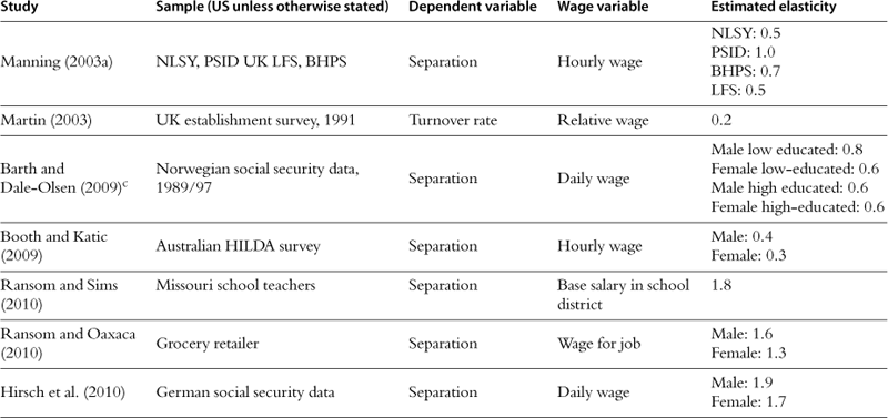
aOnly reports estimate for 1963 with average production worker wage and quit rate retrieved from original data sources.
bThese are read off from Figures B2 and B4.
cOnly OLS estimates are reported here. Some higher IV estimates for manufacturing are discussed in the text.
The earliest studies (e.g. Pencavel, 1970; Parsons, 1972, 1973) used industry data, either cross-section or time series. These estimates are probably not what good estimates of what we would like—the effect of a wage rise in a single firm—but do serve to make the point that economists have now been looking at the link between separations and wages for 40 years.
The more recent studies all use individual data but differ in a number of dimensions. First, there is the specification of the dependent variable—in some it is any separation while in others it is a “quit” defined as being a voluntary move on the part of the worker (typically self-defined). Separations that are not quits can be thought of as involuntary lay-offs—these have also been found to be sensitive to the wage, as one might expect if there is less surplus in the jobs of low-wage workers so that shocks are more likely to make employer rents negative, initiating a lay-off.
Secondly, there are differences in the way the wage variable is defined. In most studies it is simply the current hourly wage derived from the survey. A few studies use measures either of contractual wages (Ransom and Oaxaca, 2010; Ransom and Sims, 2010) or of wages workers might expect to get in the job (e.g. Meitzen, 1986; Campbell, 1993). One might expect the estimates to be sensitive to the wage measure used because we would expect the separation decision to be based not just on the current wage but future prospects as well (see Fox, 2010, for a model that explicitly models forward-looking workers). We would like to have a measure of the sensitivity of separations to a permanent change in the wage but the actual wage measures used may have a sizeable transitory component or measurement error that would be expected to attenuate elasticities. The one study that seeks to instrument the wage (Barth and Dale-Olsen, 2009)—using employer characteristics associated with higher wages—finds that this raises the elasticity (from 0.9 to 2.4 for men and 0.5 to 0.9 for women).
Thirdly, there are differences in the other variables included in the separations equations. Omitted variables, correlated with the wage, will obviously bias estimates. One potential source of problems in estimating the separation elasticity is a failure to control adequately for the average level of wages in the individual’s labor market. Separations are likely to depend on the wage relative to this alternative wage so that a failure to control for the alternative wage is likely to lead to a downward bias on the wage elasticities. On the other hand, we would expect separations to be more sensitive to the permanent component of wages than to the part of wages that is a transitory shock or measurement error. In this case, the inclusion of controls correlated with the permanent wage is likely to reduce the estimated wage elasticity. Manning (2003a,b, chapter 4) investigates this and finds that, for a number of US and UK data sets, the inclusion of standard human capital controls does not make much difference to the estimated wage elasticities.
However, one variable whose inclusion or exclusion makes a lot of difference to the apparent estimated wage elasticity is job tenure16. The inclusion of job tenure always reduces the estimated coefficient on the wage, as high-tenure workers are less likely to leave the firm and are more likely to have high wages. There are arguments both for and against the inclusion of job tenure. One of the benefits of paying high wages is that tenure will be higher, so that one needs to take account of this endogeneity of tenure if one wants the overall wage elasticity when including tenure controls: in this situation, excluding tenure may give better estimates17. On the other hand, if there are seniority wage scales, the apparent relationship between separations and wages may be spurious. Some studies that attempt to deal with this last problem are Ransom and Sims (2010), which uses the base wage in the school district as their wage measure, or Ransom and Oaxaca (2010), which uses the contractual wage for the job.
Table 6 reports estimates of the wage elasticity of separations from a number of studies. There is considerable variation in the estimates from a low of about 0.4 to a high of about 2. There are of course an enormous number of reasons for why the estimates might vary from differences in the sample to differences in the specification and no attempt is made in Table 6 to measure all the dimensions in which the studies differ.
But, there is perhaps a suggestion that those studies which have higher quality information on contemporaneous wages (e.g. from social security data) or use measures of contractual wages find elasticities in the region 1.5-2, while those with elasticities well below 1 generally just use standard self-reported measures of wages.
The bottom line from these studies is that while wages do undoubtedly affect quit rates, worker mobility does not appear to be hugely sensitive to the wage, with the highest reported elasticity being about 4 and most being well below 218. On its own this does not imply that the wage elasticity of labor supply to an employer is low because, as (25) makes clear, we also need the recruitment elasticity. But, as the next section makes clear, we would expect the recruitment and separation elasticities to be closely related to each other.
4.3.3 The link between separation and recruitment elasticities
The studies that have used the separations elasticity to estimate the elasticity of labor supply to the individual employer have all equated the recruitment elasticity to the separation elasticity, essentially using the formula in (25) to double the separation elasticity to get an estimate of the elasticity of labor supply to an individual employer. Equating the quit and recruitment elasticities was first proposed in Manning (2003b) and attracts a certain amount of suspicion, some suspecting it something of a sleight of hand. In fact, there are good reasons to believe it a reasonable approximation for separations to other jobs and recruits from other jobs. The reason is that when a worker leaves employer A for employer B because B offers a higher wage, this is a worker who is recruited to B because it is paying a higher wage than A.
To illustrate the robustness of the idea a more general result is shown here, using the generalized model of monopsony in which employers can also influence their supply of labor by spending more resources on recruitment. Assume that job offers arrive at a rate λ and that the distribution of wages in those job offers is g(x). Furthermore, assume that a worker who is currently paid w and who receives a job offer of x will leave with a probability ![]() . If the wage is the only factor in job mobility decision this will be one if x is above w and zero if it is below, but it is probably more realistic to think of it as a differentiable function. The assumption that it is only the relative wage that matters is the critically important assumption for what follows, but it is not an unreasonable assumption. If this condition was not satisfied, one would expect, as average wages rise, separations to trend up or down which they do not. Define
. If the wage is the only factor in job mobility decision this will be one if x is above w and zero if it is below, but it is probably more realistic to think of it as a differentiable function. The assumption that it is only the relative wage that matters is the critically important assumption for what follows, but it is not an unreasonable assumption. If this condition was not satisfied, one would expect, as average wages rise, separations to trend up or down which they do not. Define ![]() to be the elasticity of
to be the elasticity of ![]() with respect to its argument—we will call this the wage-specific quit elasticities.
with respect to its argument—we will call this the wage-specific quit elasticities.
Consider a firm that pays wage, w. The overall separation rate will be given by:
![]() (26)
(26)
Appendix C then proves the following result:
Result 1: The elasticity of the separation rate with respect to the wage is given by:
![]() (27)
(27)
where gs(x; w) is the share of separations in a firm that pays w that go to a firm that pays x i.e.
 (28)
(28)
Proof. See Appendix C.
Equation (27) says that the overall separation elasticity can be thought of as a weighted average of the wage-specific elasticities, where the weights are the shares of quits to firms with different wages.
To derive the elasticity of recruits with respect to the wage we need to think about the distribution of wage offers, G(w). This will be influenced by the distribution of wages across firms—which we will denote by f (w) and, we will assume, the hiring activity of firms. If H(w) is the amount of resources spent on hiring by a firm that pays w, then we will assume that the distribution of wage offers is given by:
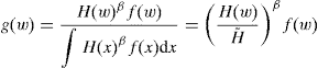 (29)
(29)
where:
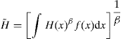 (30)
(30)
is an index of aggregate hiring activity. It is natural to assume that λ, the job offer arrival rate, depends on ![]() , the aggregate hiring activity, as well as other factors (e.g. the intensity of worker job search). The parameter β is of critical importance as it measures whether marginal costs of recruitment are increasing (β < 1) or decreasing (β > 1) in the level of recruitment.
, the aggregate hiring activity, as well as other factors (e.g. the intensity of worker job search). The parameter β is of critical importance as it measures whether marginal costs of recruitment are increasing (β < 1) or decreasing (β > 1) in the level of recruitment.
Now, consider recruitment. The flow of recruits to a firm that pays w and recruits at intensity H can be written as:
![]() (31)
(31)
where N(x) is employment in a firm that pays x. Note the multiplicative separability in (31). From this we have that:
Result 2: The elasticity of the recruitment rate with respect to the wage is given by:
![]() (32)
(32)
where:
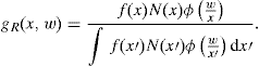 (33)
(33)
Is the density of recruits to a firm that pays w from firms that pay x.
Proof. See Appendix C.
Comparing (28) and (32) one can see the inevitable link between the quit elasticity and the recruitment elasticity—they are both averages of the wage-specific elasticities. The quit elasticity for a firm that pays w is a weighted average of the elasticity of quits to firms that pay other wages with the weights being the share of quits that go to these firms. The recruitment elasticity for a firm that pays w is a weighted average of the elasticity of quits from firms that pay other wages to firms that pay w with the weights being the share of recruits that come from these firms. If this function was isoelastic then quit and separation elasticities have to be equal, though this is impossible as ϕ has to be between zero and one. However, a further result shows how they must be linked.
For an individual firm the quit and recruitment elasticity will not generally be the same but, averaging across the economy as a whole they must be.
Result 3: The recruit-weighted recruitment elasticity must be equal to the recruit-weighted quit elasticity i.e.:
![]() (34)
(34)
Proof. See Appendix C.
The intuition for this result is simple—every quit from one employer to another is a recruit for the other employer.
Now consider what this implies about the labor supply to a firm in the long-run. For a firm that has hiring resources of H and pays a wage w, (31) implies we have that:
![]() (35)
(35)
And the elasticity of n(w) with respect to the wage is—using the argument given above— approximately twice the quit elasticity.
All of this discussion has been about moves between employers. One cannot applythe same approach for the elasticity of separations to non-employment and recruits from non-employment as there is no need for one to be the mirror image of the other. However, Manning (2003a) discusses how one can deal with this problem.
However, the way in which one interprets and uses this elasticity does need to be modified. Using a simple-minded model of monopsony, one would be inclined to conclude that there is an incredible amount of monopsony power in labor markets and conclude there is a massive amount of exploitation in the labor market that could, for example, be reduced by a very large increase in the minimum wage. In a later section we make clear that this is not the correct conclusion. It is the presence of hiring costs in (35) that makes the difference.
4.3.4 Hiring costs revisited
Earlier, we discussed how important it is whether there are increasing marginal costs to hiring but also emphasized how hard it is to get good estimates of this parameter. Here, we show how an estimate can be backed-out from the model described above.
Consider a firm choosing the wage and recruitment intensity to maximize steady-state profits19:
![]() (36)
(36)
Subject to the constraint that labor supply is given by (35). In this specification we are assuming that all hiring costs are recruitment costs—the equations would need modification if one also wanted to model training costs. The first-order condition for the wage is going to be:
![]() (37)
(37)
which can be re-written as the condition:
![]() (38)
(38)
So that the relationship between the wage and the marginal product is the familiar one. If, as the estimates discussed above suggest, the elasticity is low there will be a big gap between the marginal product and the wage. This then implies that employers make considerable rents from the employment relationship, so should be prepared to spend quite large amounts of money to hire workers. But, as we saw in the previous section, the estimates of the average hiring cost are, while not trivial, not enormous. What we show here is that these two facts can only be reconciled if there is a big difference between the marginal and average costs of hiring, which implies strongly diminishing returns to hiring expenditure.
To see this, consider the choice of hiring rate. From (36) and (35) this will be given by:
![]() (39)
(39)
which can be written as:
![]() (40)
(40)
So that the optimal hiring expenditure per worker is given by:
![]() (41)
(41)
Using (38) this can be re-arranged to give:
![]() (42)
(42)
The left-hand side is the ratio of total expenditure on hiring to the total wage bill. We have already discussed data on this in Section 2.1.2. We have also discussed how one can get an estimate of ε from the separation elasticities in Sections 4.3.1–4.3.3. This can then be used to give us an estimate of β, the sensitivity of recruits to hiring expenditure. The implied value is small—for example, if the elasticity is 8 (double the highest estimates of the separation elasticity) and hiring costs are 5% of the total wage bill, this implies that β = 0.4. Assume that hiring costs are less important or that labor supply to the firm is less elastic and that implies a lower value of β suggesting more strongly increasing marginal hiring costs. Our estimates of the importance of hiring costs and the wage elasticity of the labor supply curve to the firm are not sufficiently precise to be able to do anything more with (42) than some back-of-the-envelope calculations.
4.3.5 The employer size-wage effect
It is a well-documented empirical fact (Oi and Idson, 1999; Brown and Medoff, 1989; Brown et al., 1990) that large establishments pay higher wages than small establishments. A natural explanation for the ESWE is that employers face an upward-sloping supply curve of labor20. We might then expect the strength of the relationship to give us an estimate of the elasticity of that supply curve. However, there are problems with using a raw ESWE as an estimate of the elasticity of the labor supply curve to an employer (see Manning, 2003a, chapter 4) as, for example, there is little doubt that part of the raw ESWE is due to the fact that large employers have, on average, better-quality workers in both observed and unobserved dimensions. But, even so, one finds that workers moving from small to large employers make wage gains on average.
Here we derive the implications for the ESWE of the model of the previous section in which firms can get big by paying a high wage or spending a lot on recruiting. For a given target employment level, N, a firm will choose the least cost way of attaining it. Given the wage paid, a firm will have to spend the following amount on recruitment to have employment in steady-state of N: Subject to the constraint that labor supply is given by the inverse of (35):
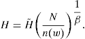 (43)
(43)
So that an employer with a target employment level of N will choose w to minimize:
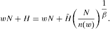 (44)
(44)
Taking the first-order condition leads to the equation:
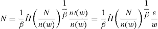 (45)
(45)
where ε is the elasticity of n(w) with respect to the wage that, for simplicity, we assume to be a constant. Taking logs and re-arranging leads to the equation:
![]() (46)
(46)
Differentiating with respect to N leads to:
![]() (47)
(47)
This is what our simple model predicts about the size of the ESWE, and one can see that it depends on the elasticity of marginal hiring costs and the elasticity of n(w). If marginal hiring costs are constant so that β = 1 , then we would not expect to see an ESWE, as firms who want to be large would simply raise hiring efforts and not wages. So, the existence of an ESWE is another piece of evidence suggesting increasing marginal hiring costs. We can go further and use empirical estimates of the ESWE to get some idea of the value of these parameters. The best estimates we have of the ESWE are quite low though these are contaminated perhaps by the difficulty of controlling for shocks to the labor supply curve that would tend to induce a negative correlation between wages and employment. Manning, (2003a, chapter 4) reports a best estimate an elasticity of wages with respect to employer size of about 0.035. Using a high value of ε of 8 (47) would then imply a value of β = 0.69. A less elastic labor supply curve would suggest a higher value of β, e.g. ε = 5 implies β = 0.80, again suggesting increasing marginal costs of hiring. These back-of-the-envelope calculations do not line up with those reported at the end of Section 4.3.4 but there should be very large standard errors attached to them.
4.4 Measuring labor market frictions
We conclude this section with a discussion of a very different approach to measuring the degree of rent-splitting. A simple yet plausible idea is that the higher the degree of competition among employers for workers, the greater will be workers’ share of the surplus. In the important and influential strand of work that sees rents in the labor market as deriving primarily from labor market frictions, the fact that it takes time for workers and employers to find each other, a natural way to capture this idea is to seek some measure of transition rates between employment and non-employment and from one employer to another.
One particular measure that has been used in the literature is the ratio of the arrival rate of job offers for an employed worker (denote this by λe) to the rate at which workers leave employment for non-employment (denote this by δ). We will denote this ratio by k. A higher value of k is more competition among employers for workers, which would be expected to raise wages. In many canonical search models e.g. Burdett and Mortensen (1998), the share of rents going to the workers can be shown to be some function of k. It can be interpreted as the expected number of job offers a worker will receive in a spell of employment (Ridder and van den Berg, 2003).
There are a lot of measures of k in the literature, with a large degree of variation. Often these estimates come from the estimation of structural models in which it is not entirely clear which features of the data play the most important role in influencing the estimates. Here, we will simply describe ways in which k can be estimated directly using data on labor market transition rates.
δ can be estimated very simply using data on the rate at which the employed leave for non-employment. λe is more complicated, as the theoretical concept is the rate at which job opportunities arrive to the employed. One might think about simply using the job-to-job transition rate, but as the employed only move jobs when the new offer is better than the current one, this is an under-estimate of the rate at which new job opportunities arise. However, in simple search models there is a mapping between the two. The reason is that if all workers always prefer high-wage to low-wage jobs and always move whenever they get a higher wage offer (however small the wage gain), then there is a simple expression for the fraction of workers G(f) who are in jobs at or below position f in the wage offer distribution. Equating inflows and outflows we have that:
![]() (48)
(48)
where u is the unemployment rate. As, in steady-state we must have that:
![]() (49)
(49)
(48) can be written as:
![]() (50)
(50)
Now the transition rate to unemployment rate is δ and the transition rate to other jobs is:
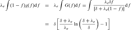 (51)
(51)
which means that the ratio of transition rates to employment relative to transition rates to non-employment is given by:
![]() (52)
(52)
This is monotonically increasing in k. In a steady-state this can be shown to be equal to the fraction of recruits who come from unemployment, a measure proposed by Manning (2003a).
One might wonder about the relationship between k and estimates of the labor supply elasticity discussed earlier in this section. In many search models there is a simple connection between the two because one can always write the profit-maximizing choice of the wage as being related to the elasticity of the labor supply curve to the firm so that k must be related to this. However, if, for example, one relaxed the assumption that it is only current or future wages that motivate job changes, then k would not seem to be a good measure of the market power of employers while an estimate of the wage elasticity still gets to the heart of the issue.
How do estimates of the balance of power between workers and employers based on this methodology compare to those based on the wage elasticity of the labor supply curve (or separations)? The advantage is perhaps that they are relatively easy to compute with nothing more than data on labor market transitions, but the disadvantage is that they are indirect (not requiring any data on actual wages) and may rely for their validity on assumptions that do not hold. For example, in these models perfect competition is the case where there is massive churning of workers, where the employer you work for one day (or hour?) has no bearing on who you work for the next. In some sense, that is a correct characterization of a perfectly competitive equilibrium, as that determines the market wage but not who of the large number of identical employers a worker works for, which is indeterminate. But, the inclusion of even a small fixed cost of changing jobs would change the prediction to one of very little turnover in an equilibrium close to perfect competition. Secondly, there is good reason to believe that not all turnover is for wage gains, which is what is relevant for employers deciding on the wage to pay. The one empirical application (Hirsch and Schumacher, 2005) does not find this measure works well in explaining variation in nurse pay across US cities.
4.5 Conclusions
This section has reviewed estimates we have of the distribution of rents in the typical employment relationship. These estimates do suggest the existence of non-trivial rents in the employment relationship. However, it is not completely clear that they are internally consistent. For example, the estimates of the rent-splitting parameter would suggest that most of the rents go to the employer. However the estimates from the actual size of rents probably suggest the workers getting most of the rents. Clearly, there is more work to be done here. While the importance of imperfect competition in labor markets might be regarded as intrinsically interesting, one still has to deal with the “so what?” question, what difference does this make to how one thinks about labor markets.
5 So what?
If there are clearly rents in the typical employment relationship, why is an imperfect competition perspective not pervasive in labor economics? There are two sorts of answers. First that it has little value-added above the perfectly competitive model—it adds more complication than insight21. This might be because perfect competition is seen as a tolerable approximation to reality so that the mistakes one makes by assuming the labor market is perfectly competitive are small. Or it might be because the comparative statics of models of imperfect and perfect competition are the same in many cases so give the same answers to many questions. For example, shifts in the demand curve and supply curve of labor will be predicted to have the same effects in perfect and imperfect competition.
The second reason why many labor economists do not adopt the perspective that the labor market is imperfectly competitive in their work is that they do not adopt any conceptual framework at all22. A well-designed and executed randomized experiment tells us about the effect of an intervention without the need for any theory or conceptual framework at all. A generation of labor economists have grown up who are not accustomed to thinking in terms of economic models at all, seeking instead good research designs. But, while estimates from randomized experiments have internal validity, their external validity is more problematic. The results tell us what happened but not why. And without at least some understanding of “why” it is difficult to draw conclusions from such studies that are of general use and enable us to make a forecast of will happen with a similar but not identical treatment in another time and place. We want to use evidence not just to understand the past but to improve the future. In practice, people do assume estimates have external validity all the time—they implicitly generalize. But perhaps it would be better if this was more explicit and we had a theory of why, and this is where an overall perspective on the workings of the labor market might help. The section that follows seeks to do just that.
6 Applications
As argued in the previous section, labor economists will probably only be convinced of the merits of thinking about labor markets through the lens of imperfect competition if they can be convinced that it makes a difference to perspectives on certain issues. In this section we review several areas in which it has been argued to make a difference, though we make no claims that this is exhaustive and we try to list others at the end.
6.1 The law of one wage
In a perfectly competitive market, the elasticity of labor supply to a single firm is perfectly elastic at the market wage for that type of worker23. Any attempt to pay a lower wage will result in a complete inability to recruit any workers at all, while any higher wage simply serves to reduce profits. As a result, all employers who employ this type of worker will pay them the same wage—the law of one wage holds. And all workers of that quality will be paid the same wage, irrespective of their reservation wage.
Those who have studied actual labor markets have often observed that the law of one wage seems to be violated, that there is, to use the jargon, equilibrium wage dispersion. Such a conclusion can be found from studies dating back to the late 1940s (e.g. Reynolds, 1946; Lester, 1946; Slichter, 1950) but more recent empirical studies all come to much the same conclusion. The existence of equilibrium wage dispersion requires some degree of imperfect competition in labor markets.
In models of imperfect competition that are based on ex post wage-bargaining, it is simple to explain the existence of equilibrium wage dispersion. Refer back to the wage Eq. (10)—this has wages depending on the specific productivity of that employer and the specific reservation wage of the worker, something that should not happen in a perfectly competitive labor market24.
In wage-posting models the most celebrated paper is Burdett and Mortensen (1998). They present a model with homogeneous workers and employers in which the only possible equilibrium is a wage distribution with no mass points. While that is an elegant and striking result, there is a very good reason for thinking it is deficient as an account of the origin of equilibrium wage dispersion. The reason is that one can track the result to an assumption of the model, which is very unappealing as an assumption about the real world and, if this assumption is made more realistic, the result collapses. That assumption is that all workers will move for the smallest gain in wages. How this delivers equilibrium wage dispersion as the only possible equilibrium can be explained with a simple diagram. Think about the labor supply curve facing an individual employer in which there is a mass of firms paying some wage w0. The labor supply curve will be discontinuous at this point so looks something like that drawn in Fig. 3. No profit-maximizing employer would then want to pay the wage w0—they would rather pay something infinitesimally higher and get a lot more workers. The mass point will unravel.
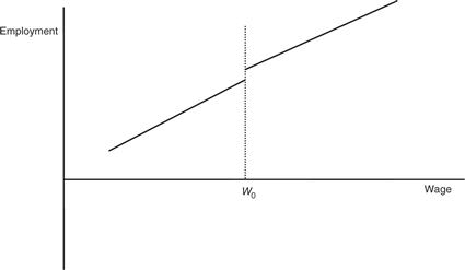
Figura 3 The labor supply to a firm in the Burdett-Mortensen model when there is a mass point at w0.
But the assumption that all workers move for the smallest gain in wages is totally implausible, so this is not a credible account of the origin of equilibrium wage dispersion. Furthermore, we do observe mass points of wages at, for example, the minimum wage and round numbers. Does this mean this type of model has no credible explanation of equilibrium wage dispersion? Far from it—the simplest and most plausible explanation is that, faced with the same labor supply curve that is always continuous in the wage, heterogeneous employers will choose to locate at different points on that supply curve. As put succinctly by Mortensen (2003, p. 6) “wage dispersion is largely the consequence of search friction and cross-firm differences in factor productivity”.
The failure of the law of one wage in labor markets has important consequences, some of which we will discuss below. It means that achieving a higher level of earnings is, in part, the result of working oneselfinto the best jobs, but that the outcome of this process will contain a considerable element of luck.
6.2 Labor market regulation
If labor markets are perfectly competitive then we know that the equilibrium will be Pareto efficient and that regulation can only be justified on distributive and not efficiency grounds. If labor markets are imperfectly competitive there is no such presumption that the market is efficient and there is at least the potential for some regulation to improve efficiency.
The labor market regulation that has received the most attention is the minimum wage. If the labor market is perfectly competitive then a minimum wage must reduce employment, as it raises the cost of labor. However, this is not necessarily the case if the labor market is imperfectly competitive. To illustrate this, we will consider the case of monopsony, though one could do the same with a matching-style model.
In the simplest model of monopsony, in which there is a single employer and the wage is the only available instrument for influencing its labor supply, there is a very simple formula relating the minimum wage to the elasticity of the labor supply to an individual employer. As we have emphasized that the labor supply to individual firms is not very sensitive to the wage, this would suggest very large potential rises in employment could be obtained from an artfully chosen minimum wage.
However, there are at least two important reasons for why such a conclusion is likely to be misleading. First, we have emphasized how the simple model of monopsony is not the best way to think about the labor market. Secondly, the model of market power we have used is a model of a single employer that ignores interactions between employers, so is only a partial equilibrium analysis.
Let’s consider the first point first. Take the model of the previous section in which the labor supply curve is given by (35) and can be influenced not just by the wage paid but also by the level of recruitment activity. To keep things simple assume the marginal revenue product of labor is constant and equal to p. First, consider the optimal employment level given the wage paid. This satisfies the first-order condition:
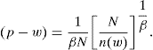 (53)
(53)
Re-arranging leads to the following “labor demand curve”:
![]() (54)
(54)
Assume, again, that n(w) is iso-elastic with elasticity ε. If the employer has a free choice of the wage we know they will choose a wage like (38). First, consider the minimum wage that will maximize employment, i.e. the wage that maximizes (54). It is easy to show that this is given by:
![]() (55)
(55)
The important point is that this is bigger than the wage that the employer will choose for itself, which will be given by:
![]() (56)
(56)
where the “m” superscript denotes the choice of a monopsonist. The log difference between the free market wage and the employment-maximizing wage is hence given by:
![]() (57)
(57)
Now consider the gain in employment from an artfully chosen minimum wage. Using (54) and the wage Eqs (55) and (56), one can show that this is given by:
![]() (58)
(58)
The standard monopsony case corresponds to the case where β = 0. This leads to the prediction of very large potential employment gains from an artfully-chosen minimum wage, e.g. even a high wage elasticity of 5 leads to a predicted employment gain of 91 log points from a wage rise of 18 log points. But if β = 0.8 this is much lower—a predicted employment gain of 9 log points from a wage rise of 3.3 log points.
The important point to note is that, unlike the simple model of monopsony, the potential gains from the minimum wage are not just influenced by the wage elasticity ε but also the parameter β, which is the relationship between average and marginal costs of hiring.
This is a partial equilibrium conclusion and not a reliable guide for policy. There are two important distinctions between partial equilibrium models of monopsony and general equilibrium models of oligopsony. First, in general equilibrium there is an important distinction between the elasticity of labor supply to the market as a whole and to individual employers. While the gap between marginal product and the wage is determined by the elasticity of the labor supply curve facing an individual employer, any employment effect will be determined by the elasticity of the labor supply curve to the labor market as a whole. There is no reason why these should be the same but it is exactly that assumption that is made by the model of a single monopsonist.
Secondly, it is important to take account of heterogeneity. There is no doubt that the minimum wage is a blunt instrument, applied across whole labor markets on employers who would otherwise choose very different wages. This means that it is almost certainly the case that the minimum wage will have different effects on employment in different employers and any measure of the impact on aggregate employment must take account of this heterogeneity. Manning (2003a, chapter 12) takes account of both these effects, showing that even in a labor market in which all employers have some market power, a minimum wage, however low, may always reduce employment.
However, models of imperfect competition are different from models of perfect competition in not making a clear-cut prediction about the employment consequences of raising the minimum wage. It is empirical studies that are important and, though this is a long debate which will not be surveyed here (see Brown, 1999, for an earlier survey), recent studies with good research designs typically fail to find any negative effects on employment for the moderate levels of minimum wages set in the US (Dube, Lester and Reich, forthcoming; Giuliano, 2009).
Although the employment effect of minimum wages has become the canonical issue in wider debates about the pros and cons of regulating labor markets, one should also recognize that models of imperfect competition in the labor market often have different predictions from competitive models about many interventions. For example, one can show that regulation to restrict aspects of labor contracts like hours or holidays can improve employment (Manning, 2003a, chapter 8). However, although imperfect competition can be used as a justification for some regulation on efficiency grounds, it always predicts some limits to regulation, with quite what those limits are left to empirical research to decide.
6.3 The gender pay gap
When Joan Robinson (1933) invented the term monopsony she used it as a potential explanation of the gender pay gap. If the labor supply of women to a firm is less elastic than that of men, then a profit-maximizing employer will choose to pay lower wages to women than men even if they have the same productivity.
A recent literature essentially builds on that observation to explain at least part of the gender pay gap. The main approach has been to see whether the separation elasticity of women is lower than that of men and then apply the logic outlined in Sections 4.3.1 and 4.3.2 to argue that this can explain some of the gender pay gap. A priori this sounds a plausible idea, as women do report that non-wage attributes are more important in their choice of a job and that they are more restricted by domestic commitments in the employment they can accept. However, this conclusion does not pop out of all the estimates. Some studies that estimate distinct separation elasticities for men and women (e.g. Barth and Dale-Olsen, 2009; Hirsch et al., 2010; Ransom and Oaxaca, 2010) do report estimates suggesting that female separation elasticities are lower than the male but this is not true of all studies (e.g. it is not true for any of the four data sets examined in Manning, 2003a, chapter 6). Perhaps worryingly, Barth and Dale-Olsen (2009) report that the estimates are sensitive to the specification used, arguing that, in their data, better specifications do deliver the conclusion that the female elasticity is below the male.
It is important to realize that a difference in separation elasticity is not necessary for models of imperfect competition to be able to explain the gender pay gap. Nor is actual wage discrimination by employers. It could simply be that women are more likely to interrupt their careers with spells of non-employment, primarily to look after young children. In a labor market where the law of one wage does not hold, this will reduce the ability of women to work themselves into and remain in the best-paying jobs. Several recent studies of the gender pay gap find that career interruptions can explain a sizeable proportion (Bertrand et al., 2009). While the most common explanation for this is that those with career interruptions accumulate less human capital, the size of the pay penalty for even small interruptions seem very large. It is not surprising that career interruptions reduce wages, but is the penalty proportionate? Research in this area needs to answer this question.
Finally, mention should be made of the effects of equal pay legislation. In the US, equal pay legislation did not seem to have an immediate effect on the gender pay gap. But, in some other countries (e.g. the UK and Australia) there was a very clear fall in the gender pay gap associated with the passing of the legislation. This change in relative wages was far more dramatic than the wage changes induced by rises in the minimum wage. If the labor market was perfectly competitive, we would expect this legislated rise in the relative wage of women to result in a fall in their relative employment. Yet, this is not what seemed to happen and Manning (1996) argues this is because the labor market has monopsonistic elements.
6.4 Economic geography
Much of economic geography is about explaining the distribution of economic activity over space—in particular, why it is so uneven, the phenomenon of agglomeration. There are many theories of agglomeration which are not reviewed here. The current literature on agglomeration tends to focus on the product market more than the labor market—but there is considerable useful research that could be done on labor market explanations.
In his classic discussion of agglomeration, Alfred Marshall (1920) speculated about possible labor market explanations, e.g. “a localized industry gains a great advantage from the fact that it offers a constant market for skill. Employers are apt to resort to any place where they are likely to find a good choice of workers with the special skill which they require; while men seeking employment naturally go to places where there are many employers who need such a skill as theirs and where therefore it is likely to find a good market. The owner of an isolated factory, even if he has access to a plentiful supply of general labor, is often put to great shifts for want of some special skilled labor; and a skilled workman, when thrown out of employment in it, has no easy refuge”.
The important point is these arguments make little sense if the labor market is perfectly competitive. In such a market the prevailing wage conveys all the information a firm or worker needs to know about the labor market25. In a perfectly competitive labor market, an employer who is small in relation to the whole market will not care about the total supply of labor to the market except insofar as it affects the prevailing level of wages. Hence, to make any sense of Marshall’s arguments, one would seem to require some degree of imperfect competition in labor markets. The formalization of Marshall’s “labor pools” theory in Krugman (1991) rests explicitly on there being a small number of employers in the labor market.
Once the labor market is monopsonistic, one can begin to make sense of some of Marshall’s arguments for agglomeration. If the labor supply curve to an individual employer is upward-sloping it makes sense to talk about a labor supply curve being “further out” because of a generally high supply of labor. One might think that monopsony models would struggle to explain agglomeration because it might be thought that an employer would like to be the only employer in an area because they would then have enormous monopsony power over the workers in that area. But that is based on a misunderstanding. Although the degree of monopsony power over the workers in an area will be high, there will be few of them and this is not to the advantage of an employer. Fig. 4 conveys this very simply. It draws two labor markets, one (the “village”) in which there are very few workers but over whom the employer has a lot of monopsony power so the labor supply curve is very inelastic. In the other (the “city’), there are more workers but less monopsony power. In which labor market will the employer choose to locate? They will choose the market where the level of employment they desire can be obtained most cheaply. So, if the desired level of employment is low, they will choose the village, while if it is high they will choose the city. Manning (forthcoming) uses this idea to explain the existence of agglomeration with employers who desire to be small locating in rural areas where they have more monopsony power and large employers locating in urban areas. And Overman and Puga (2009) investigate the implication that firms with more volatile employment will want to locate where the labor supply curve is more elastic.
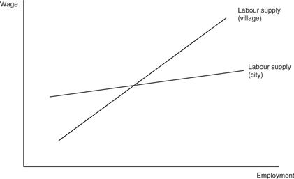
Another aspect of spatial economics that has received some attention is the estimation of commuting costs. From the perspective of a perfectly competitive labor market, one would expect workers to be fully compensated for a longer commute so that the costs of commuting can be estimated using an earnings function with the commute as an explanatory variable. But, in a labor market with frictions, we would not expect full compensation for a long commute (see Hwang et al., 1998; Manning, 2003b) so that this approach will under-estimate the cost of recruiting. An alternative approach is to use a method based on job search that worker separation rates will be based on the utility in the job and that one can get some idea of the costs of commuting by examining how wages and commute affect separations (Manning, 2003b; Van Ommeren et al., 2000). These studies often suggest a higher commuting cost, with potentially important implications for transport planning and regional development policies.
6.5 Human capital accumulation and training
Imperfection in labor markets has important implications for the incentives to acquire human capital and make investments to raise productivity. As shown by Acemoglu (1998), part of the returns to investments by workers in general human capital can be expected to accrue to future employers of the worker as the wage will be below the marginal product—this is very different from the prediction of Becker (1993) that all of the returns to general human capital will accrue to workers. The argument that workers do not fully capture the returns to investment in human capital could be used to provide a justification for the massive level of public subsidy to education that is a marked feature of all the richest economies.
Imperfect labor markets can also offer an explanation for why firms often seem to pay for the acquisition of general training by their workers—explaining this is a major problem for those who believe the labor market to be perfectly competitive. A series of papers by Acemoglu and Pischke (1998, 1999a,b) outline the theory, emphasizing the role of ”wage compression” and provide some evidence in support of that theory. They conclude that “labour market imperfections have to be an ingredient of any model attempting to understand why firms pay for general training (Acemoglu and Pischke, 1999a, p. F139).
Some other papers have found evidence supportive of their ideas. For example, Booth et al. (2004) examine the effect of the UK National Minimum Wage on training, concluding that there is no evidence it reduced the training of the affected workers (as a perfectly competitive model would predict) and some evidence that training increased. Benson (2009) investigates the reason why many hospitals sponsor students to train as nurses in local nursing schools. In a perfectly competitive labor market, this behavior would not make sense, as it is a subsidy to general training. But, in a monopsonistic labor market one can explain it as a desire of a local employer to increase its supply of labor if, as seems plausible and can be verified from the data, nurses are likely to remain in the area in which they trained. But the incentives for hospitals to subsidize nurse-training are higher where the hospital represents a higher share of nurse employment. In labor markets where there are several hospitals one might expect them to subsidize joint programs, as they have a collective interest in increasing nurse supply. Benson (2009) claims to find evidence for these predictions.
6.6 Conclusion
The list of issues, where the perspective of imperfect competition might be thought to make a difference, given above is far from exhaustive. Another chapter in this Handbook (Rogerson and Shimer, 2011) discusses potential insights of interest to macroeconomists. But there are many other labor market phenomena where imperfect competition might be thought to offer plausible explanations. Examples include the growth in wages over the life-cycle as workers try to exploit the wage dispersion in the labor market, the earnings assimilation of immigrants. Brown et al. (2008) and Hotchkiss and Quispe-Agnoli (2009) argue that monopsony can be used to explain why undocumented workers earn lower wages while the firms that employ them seem to make more profits.
What this section should have made clear is that the perspective that labor markets are pervasively imperfectly competitive has important implications for “big” questions, about the desirability and impact of labor market regulation, about the gender pay gap and about decisions about human capital accumulation. It is simply not true to claim that the perspective of perfect competition tells us all we need to know.
7 Conclusion
There are rents in the typical job. This should not be a controversial claim—workers care when they lose or get jobs, employers care when workers leave. There is more doubt about the size and distribution of those rents. A very rough benchmark might put them in the region 15%-30% of the wage, with a best guess being that most of them go to the worker. But there is undoubtedly considerable heterogeneity across jobs, the estimates have very large standard errors, and not all the evidence is mutually consistent.
The fact that there are rents in the typical job has important consequences for our view of how labor markets work and how their performance can be improved. Many empirical observations (e.g. equilibrium wage dispersion, the gender pay gap, the effect of minimum wages on employment, employers paying for general training, costs of job loss for workers with no specific skills to list only a few) that are puzzles if one thinks the labor market is perfectly competitive are simply what one might expect if one thinks the labor market is characterized by pervasive imperfect competition. One’s views of the likely effects of labor market regulation should be substantially altered once one recognizes the existence of imperfect competition. All labor economists should take imperfect competition seriously.
Appendix A Estimating the size of rents from a search model
In this Appendix we use a simplified version of the model in Section 2.2 outlined in section to derive an equation for the importance of rents to unemployed workers. The simplification is to assume that there is no on-the-job search. With this assumption the value of a job that pays w, V(w), can be written as:
![]() (59)
(59)
where δ is the rate of job loss and r the interest rate. Combining (5) and (59), and assuming r is small relative to δ we have that:
![]() (60)
(60)
which implies that:
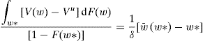 (61)
(61)
where ![]() is the average value of wages above the reservation wage. Now, consider the choice of the reservation wage, w*, which must satisfy V(w*) = Vu. From (5) and (59) we must have:
is the average value of wages above the reservation wage. Now, consider the choice of the reservation wage, w*, which must satisfy V(w*) = Vu. From (5) and (59) we must have:
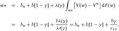 (62)
(62)
If we assume that the income when unemployed is a fraction ρ of the reservation wage then this can be re-arranged to give:
![]() (63)
(63)
which forms the basis for (8) as u/(1 – u) = δdu.
Appendix B A model with heterogeneous worker ability
Here we present a model to explain the difference in the apparent labor supply elasticity from a mandated wage increase and a mandated employment increase.
For simplicity, let us assume that the labor supply of workers of quality a (measured as efficiency units) to a firm that pays wage w, L(w, a) is given by:
![]() (64)
(64)
where we assume f(a) is a density function. A firm has to make two decisions—the wage to pay and the minimum quality worker, a*, to employ. Profits will be given by:
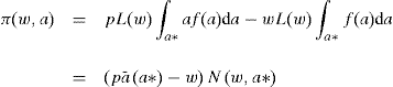 (65)
(65)
where:
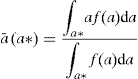 (66)
(66)
and:
![]() (67)
(67)
Now let us consider the two types of policy intervention. First, the Matsudaira type intervention. The firm is required to increase the amount of employment it has. It needs to choose (w, a*) to solve:
![]() (68)
(68)
If μ is the multiplier on the constraint, the first-order conditions for this can be written as:
![]() (69)
(69)
![]() (70)
(70)
Collecting these leads to:
![]() (71)
(71)
where ε is the elasticity of the labor supply curve, which, to keep things simple we will assume is constant. (71) gives a relationship between w and a*—denote this by a*(w).
Now consider a change in N, we will have, from the constraint in (68):
![]() (72)
(72)
which can be written as:
![]() (73)
(73)
Note that in the case where a has an exponential distribution this implies that the wage w will not change, as is found by Matsudaira. In this case:
![]() (74)
(74)
Now consider a forced change in the wage as examined by Staiger et al. (2010). The firm wants to maximize (65). This leads to the first-order condition for a* of:
![]() (75)
(75)
which can be written as:
![]() (76)
(76)
If the firm can freely choose the wage, the first-order condition for w can be written as:
![]() (77)
(77)
Now, consider a rise in the wage. We will have:
![]() (78)
(78)
In the case with the exponential distribution and for a just-binding wage this becomes:
![]() (79)
(79)
Another alternative is an effort model, then, if a denotes the effort of workers, the profit can be written as:
![]() (80)
(80)
And N = U(w)G(a), with G‘(a) < 0 reflecting the fact that workers dislike effort. This model is isomorphic to the quality model just described.
Appendix C Results equating separation and recruitment elasticity
Proof of Result 1. Simple differentiation of (26) leads to:
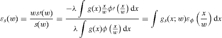 (81)
(81)
where gs(x; w) is given by:
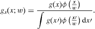 (82)
(82)
Proof of Result 2. Differentiation of (31) leads to:
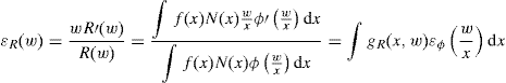 (83)
(83)
where:
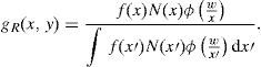 (84)
(84)
Proof of Result 3. Using (31) and the equilibrium condition that firms that pay w spend H(w) on recruitment (whatever that may be), one can write (33) as:
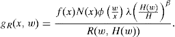 (85)
(85)
Now use (28) and reverse the roles of x and w to give:
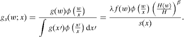 (86)
(86)
Combining (85) and (86) one obtains:
![]() (87)
(87)
Or:
![]() (88)
(88)
Now we have that:
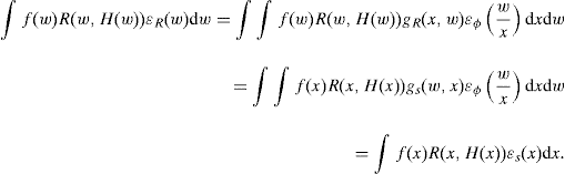 (89)
(89)
So the recruit-weighted quit and recruitment elasticities must be equal.
References
1. Abowd John M, Kramarz Francis. The costs of hiring and separations. Labour Economics. 2003;10:499–530.
2. Abowd John M, Lemieux Thomas. The effects of product market competition on collective bargaining agreements: the case of foreign competition in Canada. Quarterly Journal of Economics. 1993;108:983–1014.
3. Acemoglu Daron. Training and innovation in an imperfect labour market. Review of Economic Studies. 1998;64:445–464.
4. Acemoglu Daron, Pischke Jörn-Steffen. Why do firms train? Theory and evidence. Quarterly Journal of Economics. 1998;113(1):79–119.
5. Acemoglu Daron, Pischke Jörn-Steffen. Beyond Becker: training in imperfect labour markets. Economic Journal. 1999a;109(453):112–142.
6. Acemoglu Daron, Pischke Jörn-Steffen. The structure of wages and investment in general training. Journal of Political Economy. 1999b;107(3):539–572.
7. Albrecht James, Gautier Pieter A, Vroman Susan. Equilibrium directed search with multiple applications. Review of Economic Studies. 2006;73:869–891.
8. Angrist Joshua D, Pischke Jörn-Steffen. Mostly harmless econometrics: an empiricist’s companion. Princeton: Princeton University Press; 2008.
9. Arai Mahmood. Wages, profits, and capital intensity: evidence from matched worker-firm data. Journal of Labor Economics. 2003;21:593–618.
10. Autor David. Wiring the labor market. Journal of Economic Perspectives. 2001;15:25–40.
11. Babcock Linda, Laschever Sara. Women Don’t Ask: Negotiation and the Gender Divide. Princeton: Princeton University Press; 2003.
12. Barron John M, Berger Mark C, Black Dan A. On the Job Training. Kalamazoo, Michigan: Upjohn Institute; 1997.
13. Barron John M, Mellow Wesley. Search effort in the labor market. Journal of Human Resources. 1979;14:390–404.
14. Barth Erling, Dale-Olsen Harald. Monopsonistic discrimination, worker turnover and the gender wage gap. Labour Economics. 2009;16:589–597.
15. Beaudry, Paul, Green, David, Sand, Benjamin, 2007. Spill-overs from good jobs. NBER Working Paper No. 13006.
16. Becker Gary S. Human Capital: A Theoretical and Empirical Analysis, with Special Reference to Education, third ed., Chicago: University of Chicago Press; 1993.
17. Benson Alan. Firm-sponsored general education and mobility frictions: evidence from hospital sponsorship of nursing schools and faculty. MIT Sloan School 2009.
18. Bertrand Marianne. From the invisible handshake to the invisible hand? How import competition changes the employment relationship. Journal of Labor Economics. 2004;22:723–765.
19. Bertrand, Marianne, Goldin, Claudia, Katz, Lawrence F., 2009. Dynamics of the gender gap for young professionals in the financial and corporate sectors, Aug. 2009.
20. Bewley Truman F. Why Wages Don’t Fall During a Recession. Cambridge, Mass: Harvard University Press; 1999.
21. Bhaskar V, To Ted. Minimum wages for Ronald McDonald monopsonies: a theory of monopsonistic competition. Economic Journal. 1999;109(455):190–203.
22. Black Sandra E, Strahan Philip E. The division of spoils: rent-sharing and discrimination in a regulated industry. American Economic Review. 2001;91:814–831.
23. Blanchflower David G, Oswald Andrew J, Garrett Mario D. Insider power in wage determination. Economica. 1990;57:143–170.
24. Blanchflower David G, Oswald Andrew J, Sanfey Peter. Wages, profits, and rent-sharing. Quarterly Journal of Economics. 1996;111:227–251.
25. Blatter Marc, Muhlemann Samuel, Schenker Samuel. The costs of hiring skilled workers. University of Zurich 2009.
26. Blau Francine D, Kahn Larry M. Race and sex differences in quits by young workers. Industrial and Labor Relations Review. 1981;34:563–577.
27. William Boal M, Ransom Michael R. Monopsony in the labor market. Journal of Economic Literature. 1997;35(1):86–112.
28. Booth Alison L. The Economics of the Trade Union. Cambridge, England: Cambridge University Press; 1995.
29. Booth Alison, Arulampalam Wiji, Bryan Mark. Training and the new minimum wage. Economic Journal. 2004;114:87–94.
30. Booth Alison, Katic Pamela. Estimating the wage elasticity of labour supply to a firm: is there monopsony down-under? Australian National University: Unpublished; 2009.
31. Brenner Mark D. The economic impact of the Boston living wage ordinance. Industrial Relations. 2005;44:59–83.
32. Brown Charles. Minimum wages, employment, and the distribution of income. In: Orley Ashen-felter, Card David, eds. Handbook of Labor Economics. Amsterdam: North-Holland; 1999;2101–2163. vol. 3.
33. Brown Charles, Medoff James. The employer size-wage effect. Journal of Political Economy. 1989;97(5):1027–1059.
34. Brown Charles, Hamilton James, Medoff James. Employers Large and Small. Cambridge, Mass: Harvard University Press; 1990.
35. Brown, J. David, Hotchkiss, Julie L., Quispe-Agnoli, Myriam, 2008. Undocumented worker employment and firm survivability. Federal Reserve Bank of Atlanta Working Paper 2008–28 (December 2008).
36. Brown Donna, Dickens Richard, Stephen Machin Paul-Gregg, Manning Alan. Everything Under a Fiver: Recruitment and Retention in Lower Paying Labor Markets. London: Joseph Rowntree Foundation; 2001.
37. Bulow Jeremy, Levin Jonathan. Matching and price competition. American Economic Review 2006;652–668.
38. Burdett Kenneth, Mortensen Dale T. Wage differentials, employer size, and unemployment. International Economic Review. 1998;39(2):257–273.
39. Cahuc Pierre, Postel-Vinay Fabien, Robin Jean-Marc. Wage bargaining with on-the-job search: theory and evidence. Econometrica. 2006;74:323–364.
40. Campbell C. Do firms pay efficiency wages? Evidence with data at the firm level. Journal of Labor Economics. 1993;11:442–470.
41. Card David, Chetty Raj, Weber Andrea. Cash-on-hand and competing models of intertemporal behavior: new evidence from the labor market. Quarterly Journal of Economics. 2007;122:1511–1560.
42. Card, David E., Devcienti, Francesco, Maida, Agata, 2010. Rent-sharing, holdup, and wages: evidence from matched panel data. NBER Working Paper No. 16192.
43. Card David E, Krueger Alan B. Myth and Measurement: The New Economics of the Minimum Wage. Princeton: Princeton University Press; 1995.
44. Christofides Louis N, Oswald Andrew J. Real wage determination and rent-sharing in collective bargaining agreements. Quarterly Journal of Economics. 1992;107:985–1002.
45. Clark Andrew, Oswald Andrew. Unhappiness and unemployment. Economic Journal. 1994;104:648–659.
46. Clotfelter Charles, Glennie Elizabeth, Ladd Helen, Vigdor Jacob. Would higher salaries keep teachers in high-poverty schools? Journal of Public Economics. 2008;92:1352–1370.
47. Coles Melvyn G, Smith Eric. Marketplaces and matching. International Economic Review. 1998;39(1):239–254.
48. Currie Janet, McConnell S. Firm-specific determinants of the real wage. Review of Economics and Statistics. 1992;74:297–304.
49. DellaVigna Stefano, Daniele Paserman M. Job search and impatience. Journal of Labor Economics. 2005;23:527–588.
50. Dube Arindrajit, Freeman Eric, Reich Michael. Employee replacement costs. Berkeley: University of California; 2010.
51. Dube Arindrajit, Lester T William, Reich Michael. Minimum wage effects across state borders: estimates using contiguous counties. Review of Economics and Statistics 2010.
52. Dube Arindrajit, Naidu T Suresh, Reich Michael. The economic effects of a citywide minimum wage. Industrial and Labor Relations Review. 2007;60:522–543.
53. Ebrahimy Ehsan, Shimer Robert. Stock-flow matching. Journal of Economic Theory. 2010;145:1325–1353.
54. Eckstein Zvi, van den Berg Gerard. Empirical labor search: a survey. Journal of Econometrics. 2006;136:531–564.
55. Edgeworth Francis Ysidro. Mathematical Psychics: An Essay on the Application of Mathematics to the Moral Sciences. London: London School of Economics and Political Science; 1932.
56. Ellingsen Tore, Rosen Asa. Fixed or flexible? Wage setting in search equilibrium. Economica. 2003;70:233–250.
57. Elsby, Michael, Michaels, Ryan, 2008. Marginaljobs, heterogeneous firms, & unemployment flows. NBER Working Paper No. 13777.
58. Erens Bob, Hedges Barry. Survey of Incomes in and Out of Work. London: Social and Community Planning Research; 1990.
59. Falch Torberg. Estimating the elasticity of labor supply utilizing a quasi-natural experiment. Journal of Labor Economics. 2010a;28:237–266.
60. Falch, Torberg, 2010b. Teacher mobility responses to wage changes: evidence from a quasi-natural experiment, unpublished.
61. Farber Hank. Unions and their effects: a comparative perspective. In: Orley Ashenfelter, Card David, eds. Handbook of Labor Economics. Amsterdam: North-Holland; 2011; vol. 5.
62. Fox Jeremy. Estimating the employer switching costs and wage responses of forward-looking engineers. Journal of Labor Economics. 2010;28:357–412.
63. Galenianos Manolis, Kircher Philipp. Directed search with multiple job applications. Journal of Economic Theory. 2009;114:445–471.
64. Giuliano, Laura, 2009. Minimum wage effects on employment, substitution, and the teenage labor supply: evidence from personnel data.
65. Griffeth Rodger W, Peter W Hom, Stefan Gaertner. A meta-analysis of antecedents and correlates of employee turnover. Journal of Management. 2000;26:463–488.
66. Guiso Luigi, Pistaferri Luigi, Schivardi Fabiano. Insurance within the firm. Journal of Political Economy. 2005;113:1054–1087.
67. Hagedorn Marcus, Manovskii Iourii. The cyclical behavior of equilibrium unemployment and vacancies revisited. American Economic Review. 2008;98:1692–1706.
68. Hall, Robert E., Krueger, Alan B., 2008. Wage formation between newly hired workers and employers: survey evidence. NBER WP 14329.
69. Hall Robert E, Lazear Edward P. The excess sensitivity of layoffs and quits to demand. Journal of Labor Economics. 1984;2(2):233–257.
70. Hamermesh DanielS. Labor Demand. Princeton: Princeton University Press; 1993.
71. Hildreth Andrew KG, Oswald Andrew J. Rent-sharing and wages: evidence from company and establishment panels. Journal of Labor Economics. 1997;15:318–337.
72. Hirsch Barry T, Schumacher Edward J. Monopsony power and relative wages in the labor market for nurses. Journal of Health Economics. 1995;14:443–476.
73. Hirsch Barry T, Schumacher Edward J. Classic or new monopsony? Searching for evidence in nursing labor markets. Journal of Health Economics. 2005;24:969–989.
74. Hirsch Boris, Schrank Tomas, Schnabel Claus. Differences in labor supply to monopsonistic firms and the gender pay gap: an empirical analysis using linked employer-employee data from germany. Journal of Labor Economics. 2010;28:291–330.
75. Holzer Harry J. Job search by employed and unemployed youth. Industrial and Labor Relations Review. 1987;40:601–611.
76. Holzer Harry J. Search method use by unemployed youth. Journal of Labor Economics. 1988;6:1–20.
77. Hornstein, Andreas, Krusell, Per, Violante, Giovanni L., 2006. Frictional wage dispersion in search models: a quantitative approach. CEPR Discussion Papers 5935.
78. Howes Candace. Living wages and retention of homecare workers in San Francisco. Industrial Relations. 2005;44:139–163.
79. Hotchkiss, Julie L., Quispe-Agnoli, Myriam, 2009. Employer monopsony power in the labor market for undocumented workers. Federal Reserve Bank of Atlanta Working Paper 2009–14a (revised June 2009).
80. Hwang Hae-shin, Mortensen Dale T, Reed Walter R. Hedonic wages and labor market search. Journal of Labor Economics. 1998;16(4):815–847.
81. Jacobson Louis S, LaLonde Robert J, Sullivan Daniel S. Earnings losses of displaced workers. American Economic Review. 1993;83(4):685–709.
82. Kircher Philipp. Efficiency of simultaneous search. Journal of Political Economy. 2009;117:861–913.
83. Kleiner Morris, Won Park Kyoung. Battles among licensed occupations: analysing government regulations on labor market outcomes for dentists and hygienists. University of Minnesota 2010.
84. Klepinger Daniel H, Johnson Terry R, Joesch Jutta M. Effects of unemployment insurance work- search requirements: the Maryland experiment. Industrial and Labor Relations Review. 2002;56:3–22.
85. Kramarz Francis, Michaud Marie-Laure. The shape of hiring and separation costs in France. Labour Economics. 2010;17:27–37.
86. Krueger Alan B, Mueller Andreas. Job search and unemployment insurance: new evidence from time use data. Journal of Public Economics. 2010;94:298–307.
87. Krugman Paul A. Geography and Trade. Cambridge, Mass: MIT Press; 1991.
88. Kuhn Peter, Skutterud Mikal. Internet job search and unemployment durations. American Economic Review. 2004;94:218–232.
89. Lancaster Tony, Chesher Andrew. An econometric analysis of reservation wages. Econometrica. 1983;51:1661–1676.
90. Lakhani Hyder. The effect of pay and retention bonuses on quit rates in the US army. Industrial and Labor Relations Review. 1988;41:430–438.
91. Lazear, Edward P., 2003. Firm-specific human capital: a skill-weights approach. NBER Working Paper No. W9679.
92. Lazear Edward P, Shaw Kathryn L. The Structure of Wages: An International Comparison. Chicago: University of Chicago Press; 2009.
93. Lester Richard A. Wage diversity and its theoretical implications. The Review of Economic Statistics. 1946;28(3):152–159.
94. Lewis Michael. Liar’s Poker. London: Coronet Books; 1989.
95. McDonald Ian M, Solow Robert M. Wage bargaining and employment. American Economic Review. 1981;71:896–908.
96. Machin Stephen J, Manning Alan. A test of competitive labor market theory: the wage structure among care assistants in the south of England. Industrial and Labor Relations Review. 2004;57:371–385.
97. Manning Alan. The equal pay act as an experiment to test theories of the labour market. Economica. 1996;63(250):191–212.
98. Manning Alan. Monopsony in motion: imperfect competition in labor markets. Princeton: Princeton University Press; 2003a.
99. Manning Alan. The real thin theory: monopsony in modern labour markets. Labour Economics. 2003b;10:105–131.
100. Manning Alan. A generalised model of monopsony. Economic Journal. 2006;116:84–100.
101. Manning, Alan, 2009. A little collusion can go a long way.
102. Manning Alan. The plant size-place effect: monopsony and agglomeration. Journal of Economic Geography 2010.
103. Marshall Alfred. Principles of Economics: an Introductory Volume. 8 London: Macmillan; 1920.
104. Martin Christopher. Explaining labour turnover: empirical evidence from UK establishments. Labour. 2003;17:391–412.
105. Mas Alex. Pay, reference points, and police performance. Quarterly Journal of Economics. 2006;121:783–821.
106. Matsudaira Jordan. Monopsony in the labor market for nurses: evidence from minimum staffing legislation in California. Cornell University 2009.
107. Meitzen Mark E. Differences in male and female job-quitting behavior. Journal of Labor Economics. 1986;4:151–167.
108. Moen Espen R. Competitive search equilibrium. Journal of Political Economy. 1997;105(2):385–411.
109. Moscarini, Giuseppe, Postel-Vinay, Fabien, 2008. The timing of labor market expansions: new facts and a new hypothesis. NBER Macroeconomics Annual.
110. Mortensen Dale T. Job search and labor market analysis. In: Orley Ashenfelter, Layard Richard, eds. Handbook of Labor Economics. Amsterdam: North-Holland; 1986;849–919. vol. 2.
111. Mortensen DT. Wage Dispersion: Why Are Similar Workers Paid Differently? Cambridge Mass: MIT Press; 2003.
112. Mortensen Dale T, Pissarides Christopher A. Job creation and job destruction in the theory of unemployment. Review of Economic Studies. 1994;61(3):397–415.
113. Mortensen Dale T, Pissarides Christopher A. New developments in models of search in the labor market. In: Orley Ashenfelter, Card David, eds. Handbook of Labor Economics. Amsterdam: North- Holland; 1999;2567–2627. vol. 3B.
114. Nagypal, Eva, 2005. On the extent of job-to-job transitions.
115. Naidu Suresh. Recruitment restrictions and labor markets: evidence from the post-Bellum US South. Journal of Labor Economics. 2010;28:413–445.
116. Niederle Muriel. Competitive wages in a match with ordered contracts. American Economic Review. 2007;97:1957–1969.
117. Neal Derek A. Industry-specific human capital: evidence from displaced workers. Journal of Labor Economics. 1995;13(4):653–677.
118. Nickell Stephen J. Dynamic models of labor demand. In: Ashenfelter O, Layard R, eds. Handbook of Labor Economics. 1986.
119. Nickell Stephen J, Wadhwani Sushil. Insider forces and wage determination. Economic Journal. 1990;100:496–509.
120. Oi Walter. Labor as a quasi-fixed factor. Journal of Political Economy. 1962;70:538–555.
121. Oi Walter Y, Idson Todd L. Firm size and wages. In: Orley Ashenfelter, Card David, eds. Handbook of Labor Economics. Amsterdam: North-Holland; 1999;2165–2214. vol. 3B.
122. Overman, Henry G., Puga, Diego, 2009. Labor pooling as a source of agglomeration: an empirical investigation, LSE.
123. Oyer, Paul, Schaefer, Scott, 2011. Personnel economics: hiring and incentives. In: Ashenfelter, O., Card, D. (Eds.), Handbook of Labor Economics, vol. 4b. pp. 1769–1823.
124. Parsons Donald O. Specific human capital: an application to quit rates and layoff rates. Journal of Political Economy. 1972;80(6):1120–1143.
125. Parsons Donald O. Quit rates over time: a search and information approach. American Economic Review. 1973;63:390–401.
126. Pencavel John H. An Analysis of the Quit Rate in American Manufacturing Industry. Princeton: Industrial Relations Section. Princeton University; 1970.
127. Pissarides Christopher A. Short-run equilibrium dynamics of unemployment vacancies, and real wages. American Economic Review. 1985;75(4):676–690.
128. Pissarides Christopher A. Search unemployment with on-the-job search. Review of Economic Studies. 1994;61:457–475.
129. Pissarides Christopher A. Equilibrium Unemployment Theory. Cambridge, Mass: MIT Press; 2000.
130. Pissarides Christopher A. The unemployment volatility puzzle: is wage stickiness the answer? Econometrica. 2009;77:1339–1369.
131. Poletaev Maxim, Robinson Chris. Human capital specificity: evidence from the dictionary of occupational titles and displaced worker surveys 1984–2000. Journal of Labor Economics. 2008;26:387–420.
132. Postel-Vinay Fabien, Robin Jean-Marc. Wage dispersion with worker and employer heterogeneity. Econometrica. 2002;70:2295–2350.
133. Priest George. Timing “disturbances” in labor market contracting: Professor Roth and the effects of labor market monopsony. Journal of Labor Economics. 2010;28:447–472.
134. Ransom Michael, Oaxaca Ronald. Sex differences in pay in a “new monopsony” model of the labor market. Journal of Labor Economics. 2010;28:267–289.
135. Ransom Michael, Sims David. Estimating the firm’s labor supply curve in a “new monopsony” framework: school teachers in Missori. Journal of Labor Economics. 2010;28:331–355.
136. Reich Michael, Hall Peter, Jacobs Ken. Living wage policies at the San Francisco airport: impacts on workers and businesses. Industrial Relations. 2005;44:106–138.
137. Reynolds Lloyd G. Wage differences in local labor markets. American Economic Review. 1946;36(3):366–375.
138. Reynolds Lloyd G. The Structure of Labor Markets: Wages and Labor Mobility in Theory and Practice. New York: Harper and Brothers; 1951.
139. Ridder Geert, van den Berg Gerard. Measuring labor market frictions: a cross-country comparison. Journal of the European Economic Association. 2003;1:224–244.
140. Robinson Joan. The Economics of Imperfect Competititon. London: Macmillan; 1933.
141. Search in macroeconomic models of the labor market. In: Ashenfelter, O., Card, D. (Eds.), Handbook of Labor Economics, vol. 4a. pp. 619–700.
142. Rogerson Richard, Shimer Robert, Wright Randall. Search-theoretic models of the labor market: a survey. Journal of Economic Literature. 2005;43:959–988.
143. Rose Nancy L. Labor rent sharing and regulation: evidence from the trucking industry. Journal of Political Economy. 1987;95:1146–1178.
144. Royalty Anne Beeson. Job-to-job and job-to-nonemployment turnover by gender and education level. Journal of Labor Economics. 1998;16(2):392–443.
145. Schmeider, Johannes F., 2009. Labor costs and the evolution of new establishments, unpublished.
146. Shimer Robert. On-the-job search and strategic bargaining. European Economic Review. 2006;50:811–830.
147. Silva Jose, Toldeo Manuel. Labor turnover costs and the cyclical behavior of vacancies and unemployment. Macroeconomic Dynamics. 2009;13:76–96.
148. Slichter Sumner H. Notes on the structure of wages. Review of Economic Statistics. 1950;32(1):80–91.
149. Smith Adam. The Wealth of Nations. Penguin, London: Harmondsworth; 1970.
150. Smith, Alison, Youngs, Rachel, Ashworth, Karl, McKay, Stephen, Walker, Robert, Elias, Peter, McKnight, Abigail, 2000. Understanding the impact of Jobseeker’s Allowance, Department of Social Security, Research Report No. 111.
151. Staiger Douglas, Spetz Joanne, Phibbs Ciaran. Is there monpsony in the labor market? Evidence from a natural experiment. Journal of Labor Economics. 2010;28:211–236.
152. Stigler George J. The economics of information. The Journal of Political Economy. 1961;69(3):213–225.
153. Stigler George J. Information in the labor market. The Journal of Political Economy. 1962;70(5):94–105.
154. Sullivan Daniel. Monopsony power in the market for nurses. Journal of Law and Economics. 1989;32(2):S135–78.
155. Teulings Coen, Hartog Joop. Corporatism or Competition? Labour Contracts, Institutions and Wage Structures in International Comparison. Cambridge: Cambridge University Press; 1998.
156. Van Ommeren Jos, van den Berg Gerard, Gorter Cees. Estimating the marginal willingness to pay for commuting. Journal of Regional Science. 2000;40:541–563.
157. Van Reenen John. The creation and capture of rents: wages and innovation in a panel of UK companies. Quarterly journal of economics. 1996;96:195–226.
158. Von Wachter Till, Bender Stefan. In the right place at the wrong time: the role of firms and luck in young workers’ careers. American Economic Review. 2006;96:1679–1705.
159. Von Wachter, Till, Bender, Stefan, Schmeider, Johannes, 2009. The long-term impact of job displacement in Germany during the 1982 recession on earnings, income, and employment Columbia University, Department of Economics Discussion Paper Series DP0910-07.
160. Von Wachter, Till, Manchester, Joyce, Song, Jae, 2009. Long-term earnings losses due to mass-layoffs during the 1982 recession: an analysis using longitudinal administrative Data from 1974 to 2004.
161. Viscusi W Kip. Sex differences in worker quitting. Review of Economics and Statistics. 1980;62(3):388–398.
162. Wickens MR. An econometric model of labour turnover in UK manufacturing industries, 1956–73. Review of Economic Studies. 1978;45:469–477.
1I would like to thank the editors and conference participants for their comments. And Claudia Steinwender for her research assistance.
2It is an interesting question why not all employers are recruiting all the time if the typical employment relationship has rents. Manning (2003a, chapter 10) offers an answer to this apparent conundrum—it is costly to create jobs and employers do not createjobs they do not expect to be able to fill. Vacancies, in this view, are best seen as “accidents”.
3Though, as discussed below, it may be the case that workers are not profitable from their first day because they need some training. Employers will then be most unhappy if a worker quits on the first day they become profitable, though will still be unhappy if a worker leaves on the first day if it takes time and/or money to replace them.
4It is also likely that the capital cost of having unused capital when there is an unfilled vacancy is also quite large.
5Which is given by the inverse of λ[1 – F(w*)], the rate at which job offers arrived multiplied by the fraction of them that are acceptable to the worker.
6There may well be similar studies for other countries but I have been unable to find any. Apologies to those that I missed but statistics on time spent searching are often buried in articles whose main subject is rather different.
7Hornstein et al. (2006) use observed wages to estimate rents, finding they are enormous. However, there are a considerable number of problems with their methodology so their conclusion is probably not reliable.
8Though there is some sign of cross-over (with mixed success) in recent years, e.g. Moscarini and Postel-Vinay (2008) attempt to use wage-posting models to address macroeconomic issues and wage-bargaining models have been used address issues of microeconomic concern (though more traditional labor economists often view these attempts as reinventing the wheel and not always a round one at that).
9Actually, the natural place to look for familiar models which are similar would be trade union models which typically have a bargaining model for wage determination. But the tradition in ex post wage-bargaining models of having one worker per employer tends to limit the analogy.
10Though this statement should not be taken to mean that markets as a whole with ex post wage-bargaining need be more efficient than those with wage-posting. The efficiency concept referred to here is an ex post notion and labor market efficiency is an ex ante notion.
11This is not inconsistent with the conclusions of studies like Lazear and Shaw (2009), who argue that most wage dispersion is within firms, as that is primarily about wage dispersion between managers and janitors who differ in their productivity and not among workers who might be expected to have similar levels of productivity.
12In this case wages are a mark-up on the outside option of workers, b, and it is the size of this mark-up that contains the rent-sharing parameter.
13This excludes studies like Nickell and Wadhwani (1990), and Currie and McConnell (1992) that use sales per worker as the measure of rents, as I lack information on the share of value-added in sales which would be needed to go from these estimates to the parameter of rent-sharing. It also excludes some studies that model the link between measures of rents and wages but measure rents as, for example, a rate of return on capital (e.g. Bertrand, 2004).
14One should perhaps here mention the evidence presented in Beaudry et al. (2007) of spill-overs in wages at the city level from one sector to others.
15This study uses a qualitative measure of financial performance so is not reported in Table 4.
16The word “apparent” is appropriate here because the dependence of job tenure on the wage needs to be taken account of here when estimating the full wage elasticity.
17For the studies that report estimates both including and excluding tenure, Table 7 only reports those estimates excluding tenure.
18Such a conclusion is not new—the ethnographic study of Reynolds (1951) reached a similar conclusion.
19Note that this specification assumes that the hiring resources cost the same to all firms. As hiring costs are mostly the labor of workers within the firm an alternative assumption would be to assume they are proportional to w. The evidence in Blatter et al. (2009) and Dube, Freeman and Reich (2010) suggests recruitment costs are increasing in the wage which could be argued to favor this specification.
20In a dynamic monopsony model one might also expect a relationship between wages and employment growth. This has not been explored much in the literature, but a recent paper by Schmeider (2009) does find evidence that ffaster-growing establishments pay higher wages.
21Although, there is a part of economics that sees complication as a virtue and there does seem to be a part of research on imperfect competition in labor markets that is attracted to that.
22Mention should be made here of one part of labor economics that has taken models of imperfect competition very seriously, perhaps too seriously. This is the small industry of structural modeling of the labor market. A full review will not be attempted here (see, for example, Eckstein and van den Berg, 2006), just a few observations about the pluses and minuses of this strategy. Structural models have the advantage that they can be used to make a prediction about anything. However, the problem is that one can estimate any model, however crazy (just write down its likelihood function and maximize it) so it is not clear that the predictions of these models are any good. The discussion of identification often leaves a lot to be desired, relying heavily on functional forms and arbitrary assumptions about the sources of heterogeneity in the labor market. Structural modelers often seem more interested in the technical details than in whether their model is the right model and rather unconcerned about how obviously poorly many of these models fare in dimensions other than that which is sought to be fitted to the data. My personal view is that we have, as yet, learned relatively little from these studies about the way in which labor markets operate. Others think very differently.
23Abstracting from compensating differentials.
24Though a statement like this should not be confused with the fact that the level of reservation wages and marginal products will affect the equilibrium wage in a perfectly competitive market.
25Although, it may be that, when making a relatively long-term location decision, it is not just the level but also the variability in wages that affects choices.