
10
HSPA+ Performance
Pablo Tapia and Brian Olsen
10.1 Introduction
HSPA+ is nowadays a mature network technology that has been deployed globally for a number of years. Technologies such as 64QAM, Advanced Receivers, and Release 8 Dual Cell are well adopted today in a large number of network and devices.
This chapter analyzes the performance of various HSPA+ features in live network environments with real traffic loads. The maturity of the tested networks helped achieve performance levels that are close to the theoretical expectations from the technology itself, unlike previous hardware and software versions that often presented problems and design limitations. Even so, wide variations in performance amongst different infrastructure vendors can still be noticed, as will be discussed in detail in Sections 10.3.7 and 10.4.3. In some cases, the scenarios analyzed present challenges due to coverage, traffic load, or interference, as can be expected from real network deployments.
In the various sections, several test scenarios are analyzed, including different RF environments in stationary and mobile conditions. A detailed performance analysis is offered for each scenario, focusing on special interest areas relevant to each particular case; special care is taken to analyze the behavior of the link adaptation mechanisms, which play an important role in optimizing the performance of the data transmission and thus the spectral efficiency offered by the technology.
In general, the results show that the HSPA+ technology can provide an excellent data experience both in terms of throughput – with typical downlink throughputs over 6 Mbps with a single carrier configuration – and latency (typically under 60 ms). Networks with Release 8 Dual Cell effectively double the downlink speeds, offering throughputs between 5 and 30 Mbps, and latency as low as 30 ms. These performance levels are sufficient to offer any data service available today, including real-time services which have quite stringent delay requirements.
This chapter also highlights some of the challenges that are present in real HSPA+ deployments, including throughput fluctuations both in uplink and downlink, which makes it hard to offer a consistent service experience across the coverage area. As will be discussed, some of these challenges can be mitigated by careful RF planning and optimization, while others can be tackled with proper parameter tuning. In some cases, the technology presents limitations that cannot be easily overcome with current networks and devices, as is the case of uplink noise instability due to the inherent nature of the HSUPA control mechanisms.
Another challenge that HSPA+ networks present is the delay associated with state transitions; while the connected mode latency can be very low, the transition between various Radio Resource Control (RRC) states can hurt the user experience in the case of interactive applications such as web browsing. Chapter 12 (Optimization) provides some guidelines around various RF and parameter optimizations, including tuning of the state transition parameters.
Finally, Section 10.6 provides a direct performance comparison between HSPA+ and LTE under a similar network configuration, and shows that dual-carrier HSPA+ remains a serious competitor of early versions of LTE, except in the case of uplink transmission, where the LTE technology is vastly superior.
10.2 Test Tools and Methodology
The majority of the performance measurements that are discussed in this chapter are extracted from drive tests. While network performance indicators are important to keep track of the overall network health from a macroscopic point of view, these metrics are not very useful to capture what end users really perceive. To illustrate what the HSPA+ technology can offer from a user point of view, the best course of action is to collect measurements at the terminal device.
There are many different choices of tools that collect terminal measurements, and within these tools, the amount of metrics that can be analyzed can sometimes be daunting; in this section we provide some guidelines around test methodologies that can help simplify the analysis of HSPA+ data performance.
The first step towards measuring performance is to select the right test tools. It is recommended that at least two sets of tools are used for this:
- A radio tracing tool that provides Layer 1 to Layer 3 measurements and signaling information, such as TEMS, QXDM, Nemo, or XCal. These tools can typically be seamlessly connected to devices that use Qualcomm chip sets, although the device may need a special engineering code to enable proper USB debugging ports.
- An automatic test generation tool that is used to emulate different applications automatically, such as File Transfer Protocol (FTP) or User Datagram Protocol (UDP) transfers, web browsing, pings, and so on. These tools are a good complement to the radio tracing tool and typically provide application level Key Performance Indicators (KPIs), some Layer 3 level information, and often offer options to capture IP packet traces. Example tools in this space are Spirent's Datum, Swiss Mobility's NxDroid, and AT4's Testing App. A low cost alternative to these tools is to use free application level tools, such as iPerf (for UDP) or FTP scripts, combined with Wireshark to capture Internet Protocol (IP) traces. Capturing IP packet traces is not recommended by default unless required for specific application performance analysis or troubleshooting purposes.
Once the test tools are set up it is recommended to perform a series of quick tests to verify basic connectivity and performance. These could be done using an online tool such as SpeedTest or similar, or using a specific application test tool. Test values from Section 10.3.6 can be used as a reference for expected throughput and latency values:
- UDP down and up transfers, to check that the terminal is using the HSDPA and HSUPA channels and that the speeds that are obtained are aligned with the given radio conditions.
- 32-byte pings to verify low latency. These measurements should be performed with the terminal in CELL_DCH state; the state change can be triggered by the transmission of a large chunk of data, and verified in the radio tracing tool.
Depending on the objective of the tests, it may be a good idea to lock the phone in 3G mode to avoid Inter Radio Access (IRAT) handovers and be able to measure the performance in the poorer radio conditions. During the collection phase the amount of information that can be analyzed is limited due to the real-time nature of the task, but it is nonetheless recommended to monitor specific metrics such as:
-
Received Signal Code Power (RSCP) and Ec/No
Areas with poor radio signal (RSCP below −105 dBm or Ec/No below −12 dB) can be expected to present various challenges such as low throughput, interruptions, radio bearer reconfigurations, or IRAT handovers.
-
Number of servers in the active set
Areas with many neighbors may indicate pilot pollution. In these areas it is common to observe performance degradation, sometimes caused by a large amount of HS cell changes in the area due to ping-pong effects.
-
Used channel type
If the used channel type is “Release 99” instead of HSDPA and HSUPA, there could be a problem with the network configuration: channels not activated or conservative channel reconfiguration settings.
-
Instantaneous Radio Link Control (RLC) Level Throughput
Low throughputs in areas with good radio conditions need to be investigated, since these could indicate problems with the test tools, such as server overload. If the throughputs never reach the peaks it could indicate a problem with the network configuration, for example 64QAM modulation not activated or improper configuration of the number of HS codes.
-
HS Discontinuous Transmission (DTX) or Scheduling Rate
The scheduling rate indicates the number of Transmission Time Intervals (TTIs) that are assigned to the test device. A high DTX can be indicative of excessive network load, backhaul restrictions, or problems with the test tool.
Figure 10.1 illustrates some of the most relevant metrics in an example test tool:

Figure 10.1 Key metrics to inspect during HSPA tests. Example of drive test tool snapshot
During the test care should be taken to make sure that there are no major impairments at the time of the data collection, including issues with transport, core, or even test servers. Once the data is collected, a deeper analysis should be performed to inspect items such as:
- Channel Quality Indicator (CQI) distribution.
- Throughput vs. CQI.
- Number of HS-PDSCH codes assigned.
- Downlink Modulation assignment.
- Transport block size assignment.
- HS cell change events.
- HSUPA format used (2 ms vs. 10 ms).
In addition to RSCP and Ec/No, the CQI measurement indicates the radio conditions perceived by the HSDPA device, permitting the operator to estimate the achievable throughputs over the air interface. Typical reference CQI values are 16, beyond which the 16QAM modulation is in use, and over 22 in the case of 64QAM. However, although indicative, absolute CQI values can be misleading, as will be discussed later on Section 10.3.
The throughput can be analyzed at the physical or RLC layer. The physical layer throughput provides information about the behavior of the scheduler and link adaptation modules, while the RLC throughput indicates what the final user experience is, discounting overheads, retransmissions, and so on.
The following sections analyze these metrics in detail and showcase some of the effects that can be present when testing in a real network environment. Sections 10.3.6, 10.3.7 (for single carrier), and 10.4.1 and 10.4.2 (for dual cell), present performance summaries, including reference throughput curves based on realistic expectations.
10.3 Single-Carrier HSPA+
This section discusses the performance of HSPA+ Single Carrier with 64QAM and Type 3i receivers. This configuration represents a common baseline for typical HSPA+ deployments; therefore a deep analysis of its performance can be used as a basis to understand more advanced features, such as dual cell or 2 × 2 MIMO.
Downlink 64QAM was one of the first features to be available in HSPA+ networks and devices since its definition in 3GPP Release 7 standards. It enables up to 50% faster downlink data transmissions in areas with a good Signal to Interference Ratio (SINR) thanks to a higher modulation and the utilization of bigger transport block sizes. HSPA+ mobile devices with 64QAM are capable of theoretical speeds of 21 Mbps for single carrier devices, which in practice provide around 16 Mbps of average IP level throughput in excellent radio conditions. To take full advantage of this feature it is recommended to combine it with an advanced receiver (Type 3i), that will increase the probability of utilizing the higher modulation. Section 10.5 analyzes in detail the performance gains from 64QAM and Type 3i as compared to Release 6 HSDPA.
Both these features are relatively simple to implement and are found today in all high end smartphones, as well as in many low–medium end devices.
10.3.1 Test Scenarios
The performance of HSPA+ single carrier will be analyzed over multiple radio conditions, including stationary and mobility scenarios, based on measurements from a live network.
The network was configured with one transmit and up to four receive antennas, with advanced uplink receiver features in use, including 4-Way Receive Diversity and Uplink Interference Cancellation. In the downlink direction, the HSDPA service was configured with a maximum of 14 PDSCH codes. The test device was a HSPA+ Cat 14 HSDPA (21 Mbps) and Cat 6 HSUPA (5.76 Mbps), featuring a Type 3i receiver.
The stationary results discussed in Sections 10.3.2 to 10.3.5 were obtained under various scenarios with good, mid, and poor signal strength. The most relevant metrics are discussed to illustrate different characteristics of the HSPA+ service, such as the dependency on RSCP and CQI, the assignment of a certain modulation scheme, and others.
The different RF conditions discussed correspond to typical signal strength ranges that can often be found in live networks, spanning from −80 dBm to −102 dBm of Received Pilot Signal Power (RSCP). The test results were collected during a period of low traffic to be able to show the performance of the technology independently from load effects.
Section 10.3.7 also analyzes the HSPA+ performance under mobility conditions. As will be noted, the performance in stationary conditions is usually better than in mobile conditions, where effects from fading and HS cell changes can degrade the quality of the signal. While it is important to analyze both cases, it should be noted that the majority of data customers access their services while in stationary conditions, therefore stationary results are closer to what customers can expect from the technology in practical terms.
10.3.2 Latency Measurements
There are several types of delay that can be experienced in a HSPA+ network, depending on the radio state on which the terminal initiates the data transfer: Paging Channel State (Cell_PCH), Forward Access Channel State (Cell_FACH), or Dedicated Channel State (Cell_DCH). In addition to these, there is also the delay from terminals that are in IDLE mode, however this mode is rarely utilized by modern devices which will generally be in PCH state when dormant.
The PCH or FACH delay will be experienced at the beginning of data transfers, and can be quite large: as Figure 10.2 (left) shows, the transition from FACH to DCH alone can take between 600 and 800 ms, depending on the radio conditions. On the other hand, once the HS connection is assigned, the latency can be very small, between 30 and 60 ms in networks with an optimized core network architecture. HSPA+ latency can be further reduced with newer devices such as dual-carrier capable smartphones, as will be discussed in Section 10.4.1.
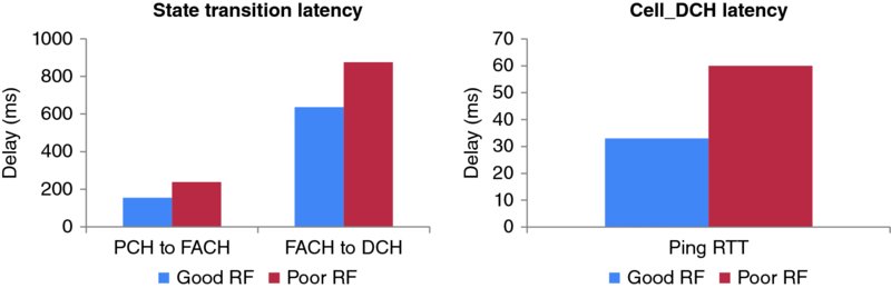
Figure 10.2 HSPA+ latency values: state transition delay (left) and connected mode latency (right)
Connection latency plays an important role in the end user experience, especially with interactive applications such as web browsing, and should be carefully optimized. One option to improve this latency is to enable direct transitions from PCH to DCH, which is shown in Figure 10.3. Section 12.2.6 in Chapter 12 discusses the optimization of RAN state transitions in more detail.
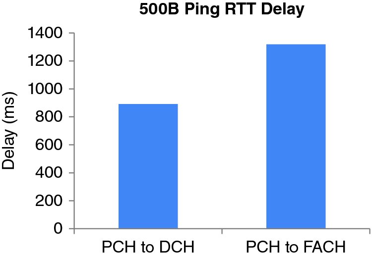
Figure 10.3 RTT improvement with direct PCH to DCH transition (left) vs. conventional PCH to FACH to DCH (right)
10.3.3 Good Signal Strength Scenario
Figure 10.4 illustrates the performance of HSDPA under good radio conditions. The pilot signal in this location was around −80 dBm, with an idle mode Ec/No of −4 dB. To simplify the presentation of the results, the measurements have been filtered to show one data sample per second.
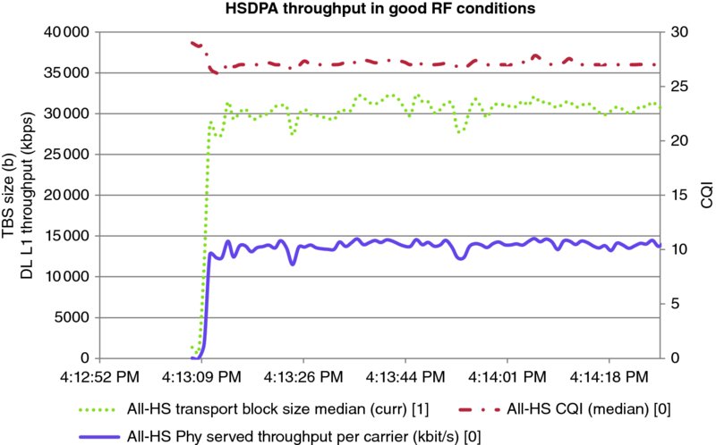
Figure 10.4 HSDPA Single-carrier performance (good radio conditions)
In these test conditions, which are good but not perfect from an RF point of view (the average CQI was around 27), the average RLC throughput obtained was 13.5 Mbps. The use of 64QAM modulation was close to 100% during this test, as expected based on the CQI.
Note that based on the reported average CQI (27), the 3GPP mapping tables indicate the use of a maximum of 12 HS-DSCH codes, and a Transport Block Size (TBS) of 21,768 bits [1]. In contrast, the UE was assigned 14 codes, with an allocated transport block size around 30,000 bits – which is close to the maximum achievable with CQI 29 (32,264 bits). In this case, the infrastructure vendor is compensating the CQI reported by the device making use of the NAK rate: the link adaptation mechanism is smart enough to realize that the device is able to properly decode higher block sizes, and is thus able to maximize the speed and spectral efficiency of the network.
The CQI measurements are defined by 3GPP to specify the reporting at the UE level, but the RAN algorithms are left open for specific vendor implementation. Furthermore, the UE reported CQI can be modified with an offset that is operator configurable, and therefore the absolute values may vary between different network operators. On the other hand, CQI can be a useful metric if all these caveats are considered, since it can provide a good indication of the Signal to Interference and Noise Ratio (SINR) perceived by the mobile at the time of the measurement.
Figure 10.5 shows a snapshot of an UDP uplink transfer in the same test location. As can be observed, the HSUPA throughput presents higher fluctuation than the downlink case, considering that the location is stationary.
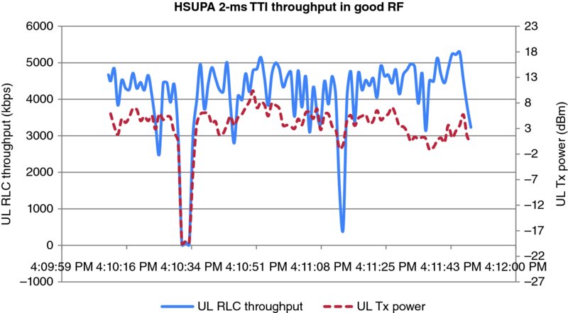
Figure 10.5 HSUPA performance in good radio conditions
The average throughput achieved in these conditions was 4.1 Mbps, with peak throughputs of up to 5.2 Mbps. The UE transmit power fluctuated between −1 and +10 dBm, with an average value of 4 dBm. During the same period, the measured RSCP fluctuated between −78 and −81 dBm, which indicates that the UL fluctuations were significantly more pronounced than any possible fluctuation due to fading.
The explanation for the HSUPA power and throughput fluctuations can be found in the nature of the HSUPA 2-ms TTI service. The power in HSUPA is controlled by two mechanisms: an uplink closed-loop power control that adjusts the power on the Dedicated Physical Control Channel (DPCCH) based on quality (UL BLER); and an UL Power assignment (grant) determined by the NodeB scheduler. The scheduling grant provides an offset for the Enhanced Dedicated Physical Data Channel (E-DPDCH) power relative to the DPCCH, which in the case of Category 6 Release 7 terminals can range between 0 (−2.7 dB) and 32 (+28.8 dB) [2]. Figure 10.6 illustrates the most relevant UL transmission KPIs for this case.
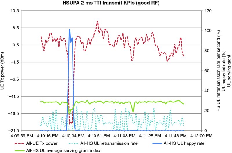
Figure 10.6 Relevant HSUPA 2-ms TTI Transmission KPIs (good RF conditions)
As can be observed, there was a period of UL inactivity (around 4:10:34) in which the UE indicated that it had no data to transmit (happy rate of 100%) – this was probably due to a problem with the test server or the tool itself. Another interesting event occurs around 4:11:08, when there is another sudden dip in throughput. At that time, the UE data buffer was full, as reflected by the happy bitrate of 0%, but the NodeB reduced the UL scheduling grant from 28 to 18, a drop of 10 dB in UE transmit power. This may have been caused by instantaneous interference, or the appearance of some other traffic in the cell. At this time, the UE throughput is limited by the allocated max transmit power.
Another source of power fluctuation is the Uplink Block Error Rate (UL BLER). In the case presented, the UE was transmitting with 2-ms TTI frames during all this time, which makes use of both Spreading Factor 2 (SF2) and SF4 channels during transmission. The data transmitted over the SF2 channels has very low error resiliency and results in a higher number of retransmissions, as can be observed in Figure 10.6: even though the overall retransmission rate is 10% across the whole test period, there are long periods in which the average retransmission rate is higher than 20%. These spikes cause the UE to transmit at a higher power, which brings the retransmission rate to a lower level and thus in turn leads to a reduction in the UE power; this cycle repeats itself multiple times during the transmission, resulting in the observed power fluctuation.
10.3.4 Mid Signal Strength Scenario
The mid signal strength scenario corresponds to the typical experience for the majority of customers. The tests in this section have been performed with a pilot strength of −92 dBm, and an idle mode Ec/No of −5 dB. As in the previous case, the tests were performed at a time when there was no significant load in the network. Under these conditions, the average downlink RLC throughput recorded was 9 Mbps. In this case, the network assigned 14 codes most of the time; as can be observed in Figure 10.7 there is a period of time when the network only assigns 13 codes, possibly due to the presence of other user traffic transmitting at the time.
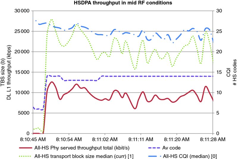
Figure 10.7 HSDPA throughput in mid RF conditions
The analysis of mid-RF level conditions is quite interesting because it permits observation of the modification of different modulation schemes (in the case of HSDPA) and transport formats (for HSUPA). In the downlink case, the RLC throughput fluctuated between 5 Mbps and 11.5 Mbps, with typical values around 8.5 Mbps. These throughput fluctuations can be explained by the commuting between 16QAM and 64QAM modulation schemes, as explained in Figure 10.8.
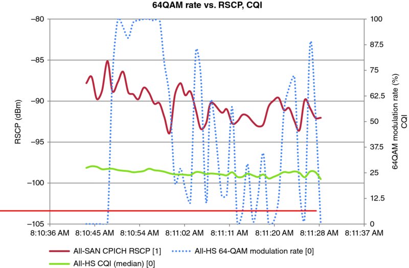
Figure 10.8 64QAM modulation assignment with changing CQI values
In this test, the fluctuations in signal strength resulted in the reported CQI swinging around 25. The 64QAM modulation was used intermittently, coinciding with CQI values of 25 or higher, with average transport block size ranges between 16,000 and 28,000 bits. As discussed earlier, the network link adaptation mechanism is not strictly following the 3GPP mapping tables, which suggests that 64QAM would only be used with CQI 26 or higher.
The HSUPA transmission in mid RF conditions also experiences throughput fluctuations due to the adaptation of the transport format block, which at this point switches between 10-ms and 2-ms TTI to compensate for the more challenging radio conditions. This effect can be observed in Figure 10.9.
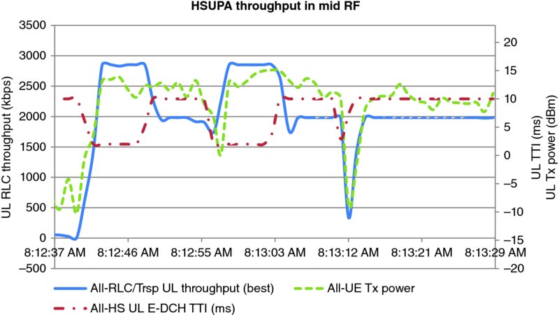
Figure 10.9 HSUPA transmission in mid RF conditions
The typical uplink RLC throughput varies between 1.8 Mbps and 2.8 Mbps, with an average throughput during the test of 2.1 Mbps. The typical UL transmit power varies between 0 and 15 dBm, with an average value of 10 dBm. Unlike in the case of HSDPA, there is no gradual degradation between transport formats. The throughput profile presents a binary shape with abrupt transitions between 10-ms TTI (2 Mbps) and 2-ms TTI (2.8 Mbps). The UE transmitted power in both cases is quite similar with, of course, more power required in the 2-ms TTI case.
10.3.5 Poor Signal Strength Scenario
This section analyzes the performance of the service under coverage limited scenarios, in which the signal strength is weak, but there's no heavy effect from interference. The RSCP in this case varied between the HSDPA case (−102 dBm) and the HSUPA case (−112 dBm).
In the case of HSDPA, the pilot strength measured during the test was around −102 dBm, with an idle mode Ec/No of −9 dB. There was some interference from neighboring cells: at times during the test up to three neighboring cells could be seen within 3 dB of the serving cell; however this didn't impact the performance significantly.
There was a significant fluctuation of signal strength at the test location, with RSCP values ranging from −107 dBm to −95 dBm. In these conditions, the HSDPA throughput experienced large variations, ranging between 2 and 6 Mbps. The changes in throughput can be explained by the fluctuations in signal strength, which can indirectly be observed in the CQI changes in Figure 10.10.
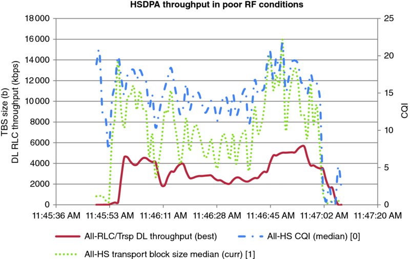
Figure 10.10 HSDPA performance in weak signal strength conditions
The performance measurements under poor RF conditions are extracted from the period with the weakest radio conditions (average RSCP of −102 dBm). In this case, the average CQI was 13, and the corresponding average throughput was 2.5 Mbps.
As in previous cases, the transport block sizes assigned were significantly higher than expected: in the worse radio conditions (CQI 13), the network assigns around 5000 bits instead of the 2288 bits from 3GPP mapping tables. Also, all 14 codes are used instead of the 4 suggested by the standards. This results in an overall improved user experience at the cell edge, in addition to significant capacity gains.
The variation in signal strength during this test permits showcasing the behavior of link adaptation when switching between QPSK and 16QAM. As Figure 10.11 illustrates, during the tests there were a few occasions when the 16QAM modulation was used; these correspond to periods when the signal strength was stronger (typically over −98 dBm), with reported CQI values over 15. The QPSK modulation was used when the CQI value remained under 15.
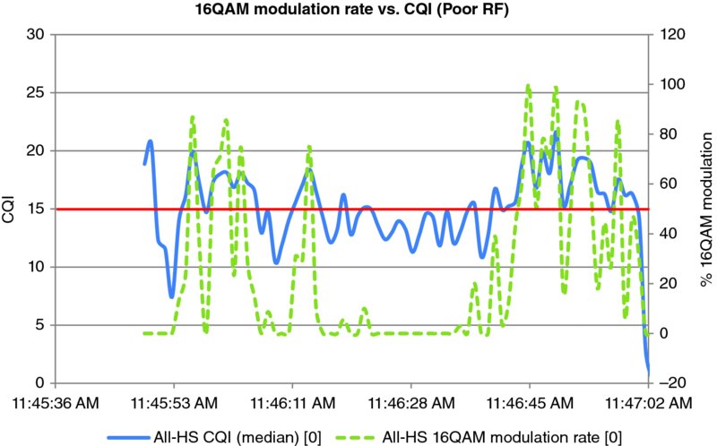
Figure 10.11 16QAM modulation assignment with changing CQI values
In the case of HSUPA, the test conditions were quite challenging, with RSCP of −112 dBm and an idle mode Ec/No of −13 dB. Under these conditions, the UE was using the 10-ms TTI transport format and transmitting at full power all the time, as shown in Figure 10.12.
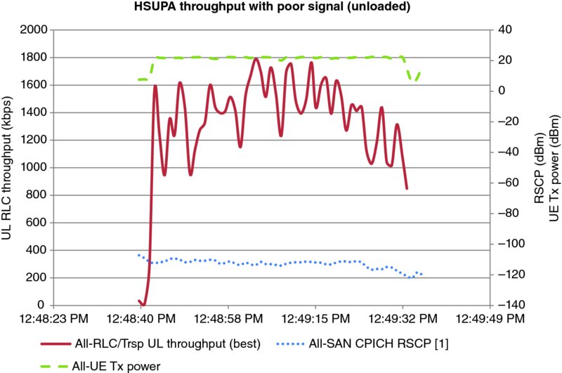
Figure 10.12 HSUPA throughput in poor signal scenario (unloaded)
The uplink throughput fluctuated between 1 and 1.8 Mbps, with an average of 1.4 Mbps during this test. While this showcases the potential of the technology, achieving such values is only possible in areas where there is lack of other interference sources, which is not typically the case.
10.3.6 Summary of Stationary Tests
The stationary tests discussed in this section illustrate the potential of the technology in real networks under low traffic conditions. Different radio conditions were tested, which enabled the illustration and discussion of network resource allocation mechanisms such as link adaptation and UL power scheduling.
In the case of HSDPA, it was noted how some infrastructure vendors tends to correct the reported CQI levels to maximize the throughput and spectral efficiency of the network, which results in a wider availability of the 64QAM and 16QAM modulation schemes, as summarized in Figure 10.13.
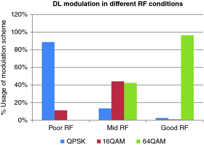
Figure 10.13 Distribution of HSDPA modulation schemes depending on radio conditions
The HSUPA throughputs reported were quite high – ranging from 1.4 Mbps in weak conditions, up to 4 Mbps in good radio conditions. However, it was observed that the uplink transmission data rate suffered severe fluctuations that may end up affecting the user experience, since applications can't predict the expected data rate. These also influence the appearance of uplink noise spikes that may lead to network congestion – this will be discussed in more detail in Section 12.2.7 of Chapter 12 (Optimization).
Table 10.1 summarizes the results from the stationary tests. The average values for both uplink and downlink are indicated, grouped by the different radio conditions.
Table 10.1 HSPA+ throughputs in stationary conditions
| Good signal strength CQI = 27.2 | Typical signal strength CQI = 25 | Poor signal strength CQI = 13.6 | |
| HSDPA | 13.5 Mbps | 9 Mbps | 2.5 Mbps |
| HSUPA | 4.1 Mbps | 2.1 Mbps | 1.4 Mbps |
As the results show, HSPA+ can provide very high throughputs even under weak signal conditions. The biggest challenges for the technology, rather than pure signal strength, are the impact from load and interference – for which Type 3i receivers can help significantly in the case of downlink transmission – and mobility related aspects. These topics will be discussed later on this chapter as well as in Chapter 12 (Optimization).
10.3.7 Drive Test Performance of Single-Carrier HSPA+
This section analyzes the performance under mobile conditions of a typical HSPA+ single-carrier network with live traffic. The tests were performed in an urban environment that wasn't heavily loaded. As in the previous sections, the tests were executed using a UDP stream to avoid side effects from TCP that may result in lower throughputs due to DTX.
Figure 10.14 illustrates the drive route and the RSCP values at different points: the darker colors correspond to higher values of RSCP, and the smaller dots indicate areas where the interference levels are high.
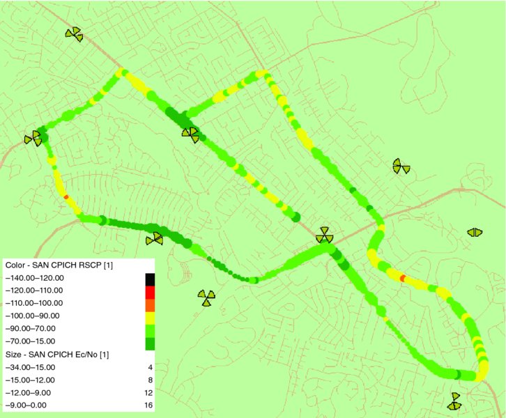
Figure 10.14 HSPA+ single-carrier drive (urban). The color of the dot represents RSCP, the size indicates Ec/No
Figure 10.15 shows the RLC throughput profile along the drive. The RLC level throughput is a realistic measurement of what the user will experience, since it does not include MAC retransmissions. As expected from a wireless network, the data speed fluctuates depending on the RF conditions, especially around handover (cell change) areas. The areas in the chart with low RLC throughput typically correspond to areas with poor coverage or high interference, and the cases where it gets close to zero are often related to problems during the HS cell change, as will be discussed later on this section.
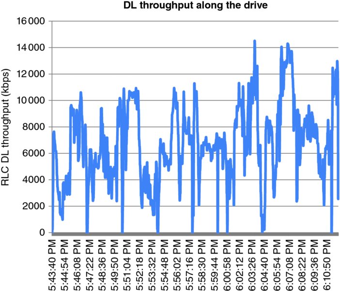
Figure 10.15 Throughput profile along the drive
The overall RLC level throughput distribution is illustrated in Figure 10.16. In this route, the throughputs are generally high, typically over 2 Mbps, with peaks of over 14 Mbps. The average throughput in this particular case was 6.7 Mbps, which is a typical value to be expected from real networks in which radio conditions are never perfect. In the same figure, a chart indicates the different modulation schemes used in this drive. In this case, 64QAM was used over 20% of the time, but more important is the fact that QPSK was only applied in 25% of the route, which corresponds to a network with good radio conditions. As discussed in Section 10.3.3, the use of the different modulation schemes greatly depends on the vendor implementation of the link adaptation algorithm. The general trend is to use as many codes as possible first, and higher order modulation after that.
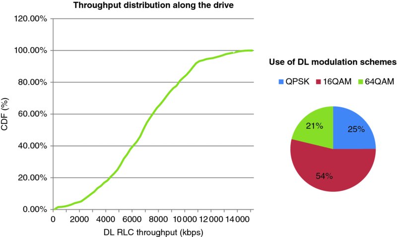
Figure 10.16 DL throughput distribution and DL modulation scheme used along the drive
Figure 10.17 summarizes the experienced RLC throughput and usage of 64QAM grouped by different RSCP ranges, to illustrate the dependency of these on the underlying radio conditions. This relationship is quite linear in typical RSCP ranges. On the same figure, the results from the stationary tests presented before are overlaid, to permit comparison between the two sets of tests.
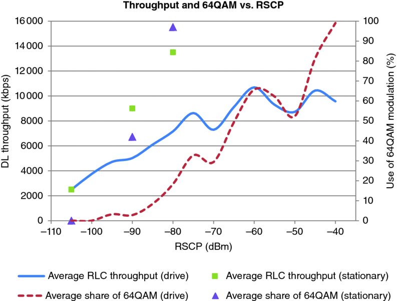
Figure 10.17 Average throughput and 64QAM usage vs. RSCP for single carrier HSPA+
Note the wide differences between throughputs and modulation share at any given radio condition between stationary and mobility tests. This indicates that the results from a drive test in an area will always provide a conservative view of what the network can really provide.
10.3.7.1 Analysis of HS Cell Changes
One of the major challenges of the HSPA+ data experience is the transition between sectors. Unlike Release 99 connections, the HS-DSCH channel doesn't have soft handover mechanisms and the data flow needs to be interrupted when the handover occurs. The HS cell change performance in HSPA+ has improved significantly since its launch, when it was common to observe data interruptions of up to several seconds during a drive. Nowadays the interruptions observed at the physical layer during the cell changes are very small (sub 100 ms) and they are often not noticed at the RLC layer. With such short interruptions HSPA+ could enable the use of real-time services such as voice over IP or live video streaming.
Figure 10.18 shows the HS-DSCH throughput profile of a call during the HS cell change. The moment of the transition can be seen based on the change of serving cell scrambling code, indicated with the darker line on the figure. Note that in the moments previous to the transition the throughput is degraded due to the interference level from the new-to-be-serving cell. The figure also shows an interruption of 60 ms in the physical layer throughput that does not impact the RLC transmission.
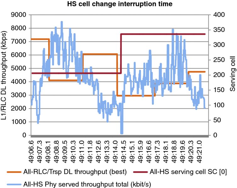
Figure 10.18 Example of HS cell change interruption time
Even though handover interruption times are not a concern anymore, in general the performance of HSPA during cell changes presents significant challenges derived from the presence of interference of the neighboring cells. As Figure 10.19 shows, the areas around the cell changes typically experience lower throughputs and larger fluctuations in general.

Figure 10.19 Throughput profile vs. HS cell changes along a drive
The presence of ping-pong effects can cause additional degradation in throughput, due to the continuous switching back and forth between sectors. Figure 10.20 shows an example in which the terminal performs multiple serving cell changes, between two sectors with scrambling codes 117 and 212. As can be observed, this ultimately brings the physical layer throughput down to zero, which impacts the subsequent RLC throughput for a few seconds after the cell change.

Figure 10.20 Ping-pong effects during a HS cell change
The cell change parameters, especially the hysteresis values, is one of the areas that need to be carefully tuned in a HSPA+ network, depending on the type of cluster and operator strategy regarding mobility. This is discussed in detail in Chapter 12 (Optimization).
10.4 Dual-Cell HSPA+
Release 8 dual cell – also called dual carrier – has been one of the most successful HSPA+ features since its commercial launch in 2010 and nowadays most high-end, as well as a significant share of medium-tier, smartphones include this feature. One of the keys to this success was the fact that this feature only required minor upgrades on the network side – in some cases purely software since multiple carriers had already been deployed for capacity purposes – and it enables the operator to compete with other networks offering Release 8 LTE services.
As discussed in Chapter 3 (Multicarrier HSPA+), 3GPP has continued developing the carrier aggregation concept, with new items in Release 9 and Release 10 such as uplink dual carrier, dual-band dual-carrier, and multicarrier aggregation; however at the time of writing this book such features were not commercially available.
The Release 8 downlink dual cell feature enables the aggregation of two adjacent UMTS carriers into a single data pipe in the downlink direction, theoretically doubling the bitrate in the entire cell footprint, and providing some efficiency gains due to trunking efficiency – although these gains are questionable in practice, and greatly depend on vendor implementation as will be discussed in Section 10.4.3.
Combining the transmission of two carriers introduces efficiencies in mobility or inter-layer management, since now load balancing across the carriers can be handled by the NodeB scheduler instead of through load based handovers. Additionally, dual-carrier networks provide larger burst sizes than two separate carriers, which improve the data user experience of the smartphone customers; this is due to the fact that typical traffic profiles are bursty in nature and rather than requiring a constant stream of high bitrate, they can benefit from having short bursts of data at high speed followed by semi-idle periods. As will be discussed in Chapter 13, on many occasions dual carrier can provide a similar experience to early versions of LTE from a user experience point of view, which will likely prolong the life of existing UMTS networks.
Figure 10.21 illustrates the maximum and typical throughputs expected from a HSPA+ dual-carrier network, as compared to a single-carrier one. The difference between maximum bitrates in the lab as compared to field measurements has to do with practical load conditions and configuration of the service, since the absolute max speeds can only be achieved when all 15 HS-SCCH codes are in use, which is not typically possible in the live network. Note that only downlink throughputs are displayed, since the uplink bitrates remain the same for single and dual carriers.
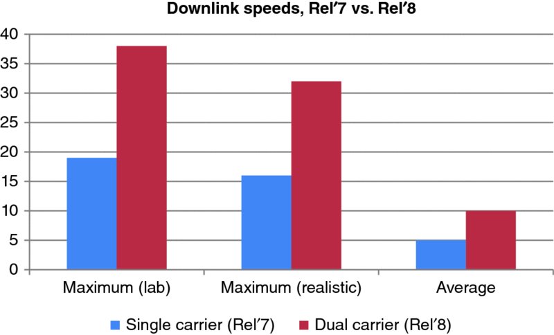
Figure 10.21 Typical downlink bitrates, dual vs. single carrier
This section presents results from stationary and drive tests in multiple live dual-carrier networks, including different vendors and traffic loads. As will be discussed, there are many factors that affect the throughput provided by the feature, which results in wide variations between different networks. Some of these factors include:
- Baseband configuration. In some networks, the lack of baseband resources can limit the number of HS codes that can be used, thus limiting the maximum throughput achievable by dual carrier.
- Vendor implementation. Some vendors treat dual-carrier users differently than single carriers, leading to a de-prioritization of scheduling resources for dual carrier, which results in lower achievable throughputs.
- Load and interference.
- Terminal performance.
10.4.1 Stationary Performance
The following results show a summary of tests performed around the network in Figure 10.25. This network was configured with two UMTS carriers in a high frequency band and presented low traffic in the sectors at the time of the tests. Several stationary tests were conducted in multiple locations, representing various RF conditions, which are reflected in the RSCP and CQI noted in Figure 10.22. These tests were conducted with a USB data stick with Type 3i receiver capabilities.
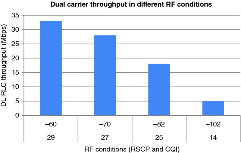
Figure 10.22 Dual carrier downlink throughput in different RF conditions (stationary)
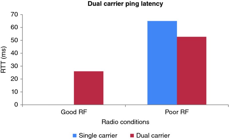
Figure 10.23 Dual carrier ping latency in good (left) and poor (right) radio conditions
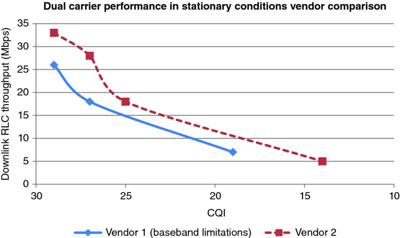
Figure 10.24 Dual carrier performance comparison between vendors (Vendor 1 with baseband limitations)

Figure 10.25 Dual carrier test metrics: Ec/No (a) and throughput (b)
As the results show, in very good RF conditions (CQI 29) the average downlink speed reported at the RLC layer was 33.4 Mbps, which is far from the theoretical maximum that the dual-carrier technology can deliver (42 Mbps). This is due to the practical limitations on configuration and usage of HS-PDSCH codes, which in this case was set to 14: with this number of codes, the maximum physical layer throughput is 32.2 Mbps according to the 3GPP mapping tables.
As discussed in Section 10.3 the infrastructure vendor adjusts the assigned transport block size and modulation, based on internal algorithms, to try and maximize the offered throughput. This will not be discussed in detail in this section, since it is the same effect illustrated in the case of single-carrier devices.
While it is possible to achieve over 30 Mbps in perfect radio conditions, in more realistic conditions, the expected downlink throughput would be lower: the value recorded in our tests was 28 Mbps for good radio conditions, while in more typical conditions it was around 18 Mbps; in areas with poorer signal strength the throughput reduces to around 5 Mbps. These results are in line with the expectation that dual-carrier devices would double the downlink throughput, which is summarized in Table 10.2 below. Note that the results are perfectly aligned, even though these were tested in different networks at different times using different devices – however the infrastructure vendor was the same.
Table 10.2 Comparison of single vs. dual carrier stationary performance
| Good RF (CQI 27) (Mbps) | Mid RF (CQI 25) (Mbps) | Poor RF (CQI 14) (Mbps) | |
| Single carrier | 13.5 | 9 | 2.5 |
| Dual carrier | 28 | 18 | 5 |
One additional benefit that can be noticed when using dual-carrier devices is a reduction of latency of up to 10 ms as compared to Cat 14 devices. There is really not a fundamental reason for this, and the improved latency is likely due to the fact that dual-carrier devices have better UE receivers and processing power. The ping tests in Figure 10.23 show that dual-carrier devices can achieve connected mode latency values as low as 26 ms in good radio conditions. In poor conditions, latency degraded down to 53 ms. A test performed in the same location with a single-carrier data stick showed average latency values of 65 ms.
Figure 10.24 compares the downlink performance of two different infrastructure vendors. One of the vendors had a limitation on the baseband units that limited the amount of codes used by the dual-carrier to a maximum of 26 (13 per carrier), while the other vendor could use up to 28 codes in this particular configuration.
As Figure 10.24 shows, in the case of the vendor with baseband limitations (Vendor 1), the maximum achievable throughput would be around 26 Mbps in perfect RF conditions, and around 15–18 Mbps in more typical conditions. Another interesting fact to note is that the link adaptation method of this vendor is more conservative than Vendor 2, thus resulting in an overall performance loss of about 20%. Further analysis of vendor performance differences will be presented in Section 10.4.3.
10.4.2 Dual-Carrier Drive Performance
The dual-carrier technology does not introduce new handover mechanisms, and it should be expected that similar link adaptation methods to those analyzed for single-carrier networks are utilized. This should result, theoretically, in a dual-carrier network offering a similar throughput profile as a single-carrier network, at twice the speed. As discussed in the previous section, it should also be expected that mobility results present worse performance than those obtained in stationary conditions, under the same radio conditions.
In this section we analyze the performance of various live dual-carrier networks through drive tests that include different load and interference conditions as well as different infrastructure networks. As will be discussed later on this section, there are significant performance differences amongst infrastructure vendors; the reference network analyzed in this case shows the vendor with the better tuned Dual Carrier Radio Resource Management (RRM) algorithms.
Figure 10.25 shows a drive route on a network in an urban environment configured with two UMTS carriers in a high frequency band, in which the traffic load was evenly distributed in both carriers. This network presented some challenges, including high traffic load, and some high interference areas as can be observed on the left chart (darker spots). The chart on the right illustrates the downlink throughput along the drive route.
The average throughput along this drive was 10.5 Mbps, with typical throughputs ranging from 2 to 20 Mbps, depending on the radio conditions. Due to the high traffic in the area, the number of HS codes per carrier available during the drive fluctuated between 11 and 14, depending on the area, with an overall average of 12 codes along the drive. Figure 10.26a shows the throughput distribution, which presents a bimodal profile that follows the RF conditions in the drive. The 64QAM modulation was used 32% of the time, as indicated in Figure 10.26b.
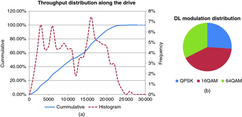
Figure 10.26 Distribution of throughput (a) and modulation schemes (b) along the drive
Both the throughput and modulation are directly related to the radio conditions. In this case, there was a high correlation between pilot strength (RSCP) and offered throughput, as illustrated in Figure 10.27. Estimating the throughput value for specific signal strengths can be quite useful to predict data performance in the network based on RF prediction or measurements, for example. As such Figure 10.27 can be used as a reference in case of a loaded network with a high noise floor.
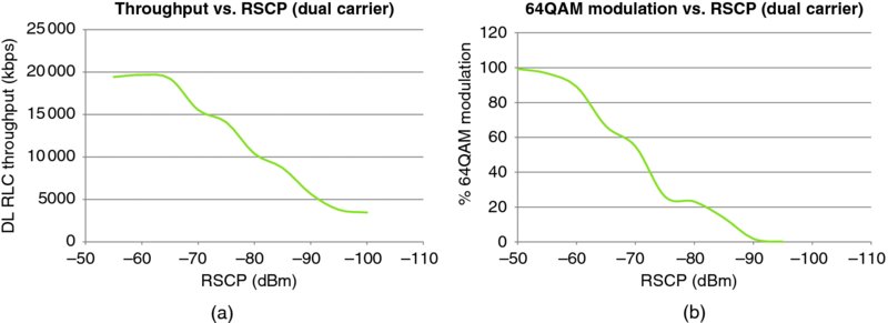
Figure 10.27 Throughput (a) and use of 64QAM modulation (b) in different radio conditions
It should be noted that the throughputs corresponding to the weaker signal strength values are low when compared to the results obtained in stationary conditions, or even compared to the single carrier results discussed in Section 3.7. This is due to higher interference levels in this network, as will be discussed later on this section.
In general, the relevant metric that is tied to throughput is link quality (CQI). An alternative method to represent the throughput performance under different radio conditions is shown in Figure 10.28. These curves isolate the performance of the specific network from the technology itself and can be used as a reference to analyze the performance of the dual-carrier technology; however, it should be considered that the absolute CQI values may differ depending on device type and vendor implementation.
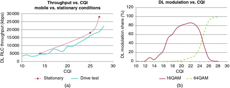
Figure 10.28 Dual carrier throughput (a) and modulation vs. CQI (b)
Figure 10.28a shows the expected throughput for various CQI values based on the test drive. The stationary measurements discussed earlier are also displayed for comparison purposes: mobility measurements tend to be lower for each particular radio condition, especially in cases of good CQI levels. Figure 10.28b illustrates the assignment of the different downlink modulation schemes, which shows that 64QAM is only utilized in the higher CQI ranges (23–30), as expected.
Figure 10.29 illustrates the throughput profile along the drive to better analyze the correlation between interference and throughput. The chart shows how the dual-carrier performance suffers in areas with high interference: while the typical throughputs along the drive were around 10 to 15 Mbps, the areas with low CQI (below 15) experienced throughputs below 5 Mbps.
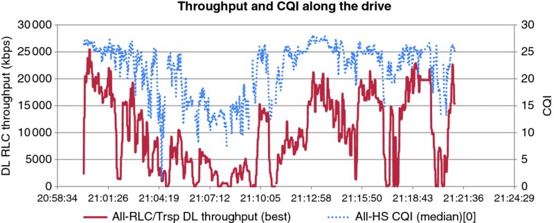
Figure 10.29 Throughput and CQI profile along the drive
The poor throughput was heavily linked to areas with weaker signal strength (RSCP) values, however the underlying problem was one of interference due to pilot pollution. Pilot pollution is a very typical situation in real deployments, especially in urban areas, and is associated with the reception of many pilots with similar signal strengths. As discussed in Section 10.3.5, HSPA+ can still provide very good performance levels even at low signal strength conditions; however, it cannot deal so well with interference, in particular when it comes from multiple cells simultaneously.
The profile also presents dips of CQI coinciding with cell change transitions, sometimes creating periods of data interruption. A detailed analysis of this situation showed that pilot signal experienced sudden power drops over a short distance, which is usually indicative of heavily downtilted antennas. In any case, these problems are not related to the network technology itself, rather to the RF planning of the network, but are a good example to highlight the importance of a proper RF planning exercise. Chapter 11 (Planning) will discuss this topic in more detail and provide guidelines and tips to properly plan and optimize the HSPA+ network.
Figure 10.30 provides a breakdown of the throughput allocated on each of the two carriers assigned to the dual-cell device during the transmission.
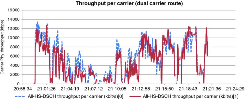
Figure 10.30 Throughput per carrier (dual-carrier transmission)
As the chart shows, the throughputs in both carriers are balanced, with minor differences in throughput (5.8 Mbps average in carrier 1 vs. 5.1 Mbps average in carrier 2), which can be explained by slightly different load and interference conditions in each carrier, as is typically the case in live networks. Note that this behavior may vary depending on vendor implementation and configuration of the traffic balancing parameters in the network.
10.4.3 Impact of Vendor Implementation
During the stationary performance discussion it was noted how there were significant performance differences with different vendor suppliers, especially in the case of hardware restrictions (e.g., baseband limitations). This section analyzes further performance differences between vendors that are rather related to the design of the radio resource management methodologies, in particular the NodeB scheduling function and link adaptation.
When analyzing the throughput profiles for two different infrastructure vendors, it was found that one vendor was outperforming the other by 20–30%, especially in the areas with mid to good radio conditions. Such a difference has a significant impact on user experience and network capacity.
The difference between both vendors can be mostly explained by the strategies around link adaptation, and in particular, the assignment of the downlink modulation schemes. As Figure 10.31 shows, the vendor with the best performance assigns both the 16QAM and 64QAM modulation schemes well before the other one.
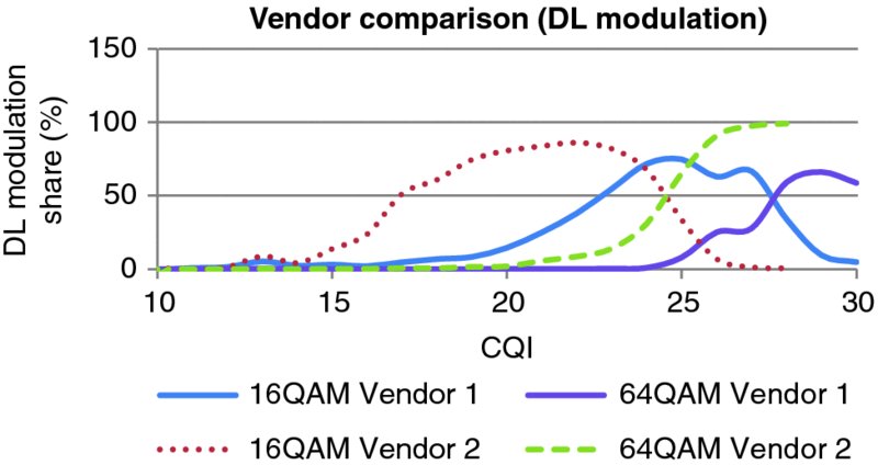
Figure 10.31 Downlink modulation assignment with different vendors
Vendor 2 starts assigning the 16QAM modulation around CQI 16, while Vendor 1 doesn't reach the same threshold until CQI 20: that is, the first vendor starts transmitting at a faster rate with approximately 4 dB worse quality than the second. While an aggressive setting of the modulation could arguably result in higher error rate, such an effect is controlled by utilizing the NAK rate in the decision-making process of the algorithm. In a similar fashion, the 64QAM modulation is available with 2 dB of worse signal quality, and more importantly the modulation is used at 100% rate when radio conditions are sufficiently good, which is not the case for the other vendor.
Furthermore, when analyzing the behavior of Vendor 1 it was found that there are additional effects that degrade the performance of the dual carrier service. The following example presents a comparison between a single carrier and dual carrier test drive in Vendor 1's network. The same device was used for the tests, changing the terminal category from 24 to 14, and the same drive route was followed (drive route from Figure 10.14). Figure 10.32 shows the throughput distribution for both the single-carrier and dual-carrier device.
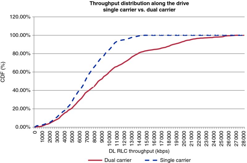
Figure 10.32 Single carrier vs. dual carrier throughput distribution
The results from this exercise show that the dual-carrier device only achieved 45% higher throughput on average as compared to the single-carrier device; and even more important, in the lower throughput ranges (poor radio conditions), there was no noticeable difference between both devices.
When analyzing the reasons behind this behavior it was noted that this vendor prioritizes the traffic from single-carrier devices over dual carrier to try and achieve the same level of QoS independently of the terminal capabilities (in other vendor implementations it is possible to select the priority of dual-carrier devices in the scheduler, rather than being hard-coded). That explains part of the problem, since the network was loaded at the time of the tests; as Figure 10.33 shows, the dual-carrier device experienced a higher DTX rate than the single-carrier one, especially in one of the carriers. A higher DTX rate indicates that the device is receiving fewer transmission turns by the HSDPA scheduler.
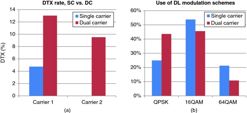
Figure 10.33 Comparison of scheduling rate (a) and DL modulation (b) for single vs. dual carrier
Another interesting aspect that can be observed from this vendor is that the assignment of the modulation scheme was significantly more conservative in the case of the dual-carrier device, as can be appreciated in Figure 10.33b: the single-carrier device makes more use of 64QAM and 16QAM than the dual-carrier device, even though the radio conditions were the same for both carriers.
In the case of the other vendor tested, the dual carrier was found to perform in line with the single-carrier performance, effectively doubling the user throughput at any point of the cell footprint. These are important performance differences that should be considered when selecting the infrastructure vendor.
10.5 Analysis of Other HSPA Features
This section analyzes some of the HSPA+ features that are commercially available in networks today, apart from Release 8 dual cell, which was reviewed in the previous section: 64QAM, advanced receivers, single-carrier MIMO, and quality of service.
At the time of writing this book it wasn't possible to test commercially available versions of other interesting features, such as dual-cell HSUPA, CS over HS, or dual-carrier MIMO. While some of these features may become commercially available in the future, it is likely that they will not be widely adopted due to the required modification and penetration of devices incorporating such features.
Other relevant HSPA+ features that are not discussed in this section include CPC, and enhanced FACH and RACH, which have already been discussed in Chapter 4.
10.5.1 64 QAM Gains
Downlink 64QAM was one of the first HSPA+ features to be commercially launched, and one that will typically be found in any HSPA+ phone. As such, all the results discussed in this chapter have assumed that this feature was available by default; however it is interesting to analyze how the feature works and what benefits it brings as compared to previous Release 6 HDSPA terminals.
The use of 64QAM can increase by 50% the peak speeds of previous HSDPA Release 6 in areas with very good signal strength and low interference. This section presents an “apples to apples” comparison of a device with and without 64QAM capability, along the same drive route. In order to make the results comparable in both cases we used exactly the same device, in which we could turn on and off the availability of 64QAM by selecting the desired UE category (Cat 14 vs. 10). The advanced receivers feature (Type 3i) was active for both device categories.
Figure 10.34 shows the signal strength along the drive route; as can be observed, there were many areas along the drive that were limited in coverage, therefore the results from this drive would provide a conservative estimate of the potential gains from the technology.
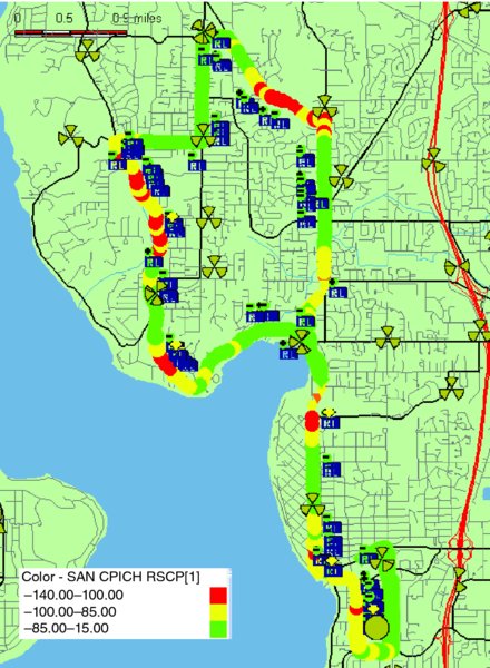
Figure 10.34 64QAM drive area
Figure 10.35 illustrates the throughput profile of both terminal configurations: Category 10 (on the left) and Category 14 (on the right). The Cat 14 device follows the same throughput envelope as the Cat 10 device; however the peaks are higher in the good throughput areas. The 64QAM device presented average throughput peaks of up to 14 Mbps as compared to the 10 Mbps registered with the Cat 10 configuration.
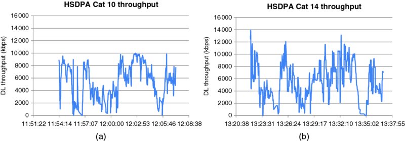
Figure 10.35 Throughput profile of Category 10 (a) vs. Category 14 terminal (b)
Figure 10.36 summarizes the availability of the 64QAM modulation along the route: the Cat 14 device was able to utilize 64QAM in 25% of samples along the route, which resulted in an overall increase in average throughput of 10% in this particular example.
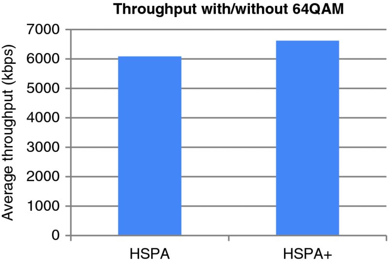
Figure 10.36 64QAM throughput gain
It should be noted that the availability of 64QAM is heavily dependent on the link adaptation method used by the infrastructure vendor, as discussed in Section 10.3.6; some infrastructure vendors apply very conservative settings which results in very low 64QAM utilization, and therefore lower capacity gains overall.
10.5.2 UE Advanced Receiver Field Results
As the HSPA+ RAN (Radio Access Network) downlink throughput continued to evolve via high order modulation and MIMO, which fundamentally only improve speeds in good SNR areas, there was a need to improve the user throughputs in poor SNR areas near the inter-cell boundary areas. These areas need to combat multi-path fading and inter-cell interference created from neighboring cells. Implementing advanced receivers in the UE (User Equipment) as discussed in more detail in Chapter 8, offers an attractive way to improve the downlink user experience in poor SNR areas and provide a more ubiquitous network experience over more of the geographical footprint with no network investment or upgrades to the RAN. Advanced receivers were first introduced into HSPA consumer devices starting around 2010. In only a few years, they have become a mainstream technology that is in nearly every new high-tier and medium-tier HSPA+ smartphone in the USA1.
One of the main challenges for operators is to provide solid in-building coverage to areas where it is historically difficult to build sites, such as in residential areas. Another practical challenge with HSPA+ is cell border areas, especially those locations where three or more pilots are present at relatively the same signal strength. In these locations, in addition to the degradation due to high interference levels, HS cell changes have a negative effect on the throughput because of the constant ping-ponging – sometimes causing interruptions in the data transmission. One of the benefits of Type 3i receivers is that the session can cancel those interference sources, and thus remain connected to the same serving cell.
Figure 10.37 shows various stationary test locations where the performance of advanced receivers was evaluated. The locations were chosen to try to represent typical coverage challenges that are experienced in residential areas and measure the range of throughput improvements that might be expected. The results from these tests using a cat 14 UE are shown in Table 10.3. The Qualcomm QXDM (Qualcomm eXtensible Diagnostic Monitor) tool was used to change the device chip set configuration from single receiver (Type 2) to receiver diversity (Type 3) and to receiver diversity with interference cancellation (Type 3i).
Table 10.3 Stationary test results with different UE receiver types
| Stationary location | RSCP (dBm) | Type 2 Rx (Mbps) | Type 3 Rx (Mbps) | Type 3i Rx (Mbps) | Type 3 over Type 2 gain (%) | Type 3i over Type 2 gain (%) |
| 1 | −60 | 10.7 | 12.0 | 13.0 | +12 | +21 |
| 2 | −80 | 8.3 | 8.9 | 9.2 | +7 | +11 |
| 3 | −100 | 2.0 | 3.4 | 4.0 | +70 | +100 |
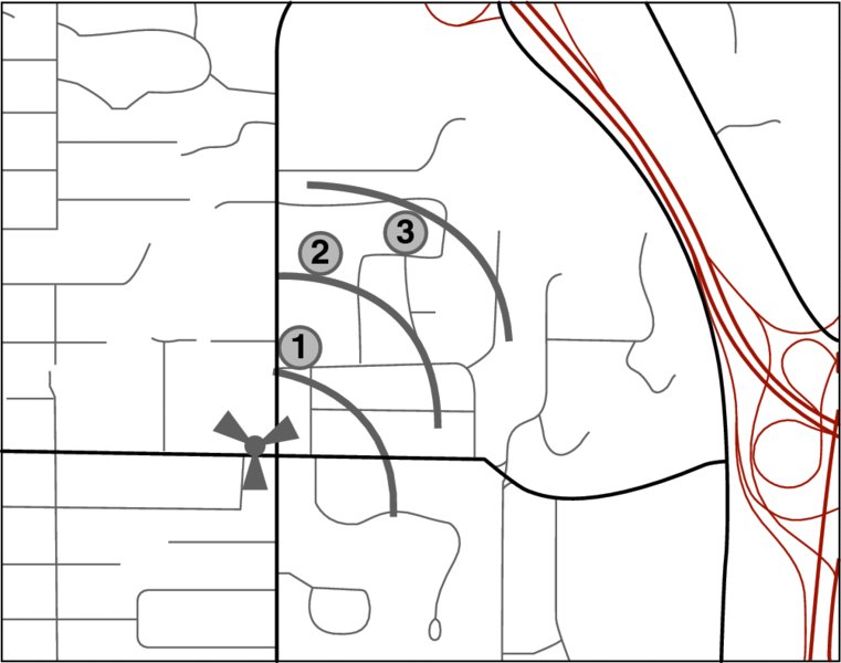
Figure 10.37 Location of stationary tests for advanced receivers
As Table 10.3 shows, the largest gain is achieved on location #3 (cell edge) and most of it is derived from implementing receiver diversity (Type 3). There is an additional improvement by implementing interference cancellation (Type 3i) too, with the largest gains also being realized near the cell edge. Location #3 in the table below had three pilots in the active set with roughly the same RSCP; however, not surprisingly, the performance improvement of interference cancellation is a function of the number of interfering pilots and the load on those neighboring cells.
The same three receiver configurations were also tested under mobile conditions, following the test route illustrated in Figure 10.38.
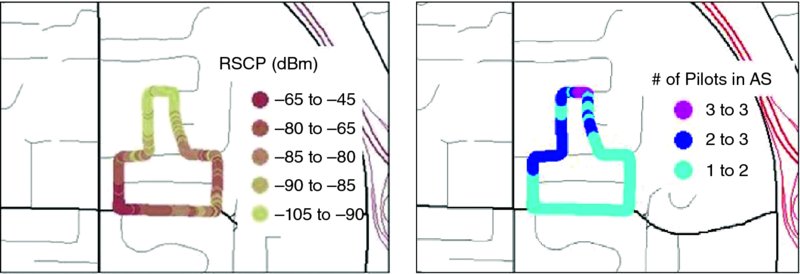
Figure 10.38 UE Advanced receiver drive route
The mobility testing drive route was chosen to represent both the good RSCP and Ec/No areas near the NodeB and also areas where there were multiple pilots, which may cause a UE to ping-pong during HS cell reselection. The area at the top of the map in particular was quite challenging because there were as many as three pilots covering this area all with an RSCP of around −100 dBm at the street level. Figure 10.39 below shows the throughput distribution for the three different test cases.
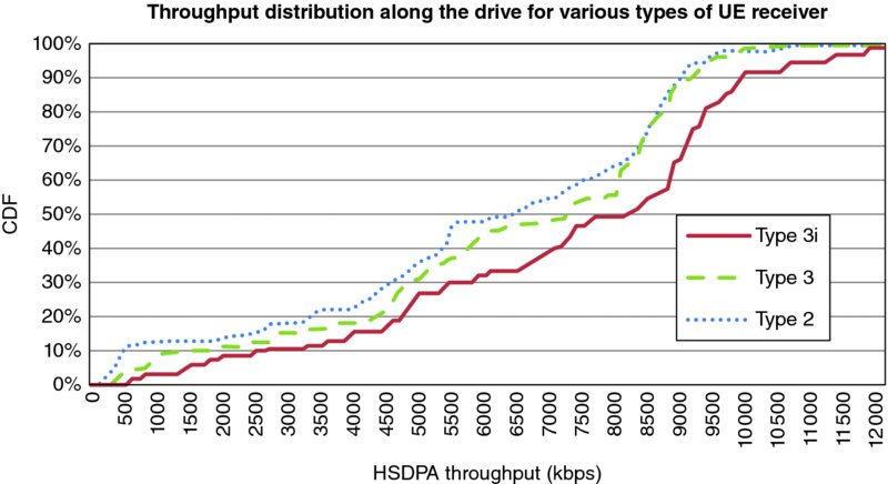
Figure 10.39 Throughput distribution for different types of UE receivers
The mobility results show again that the largest gains in throughput performance are achieved at the cell edge, which can be as high as 100%. The average gains are more modest in the 20–40% range between Type 2 and Type 3i receivers. On the higher throughput range, Type 3i provides a significant boost and enables the receiver to achieve higher peaks than with Type 3 or Type 2 configurations.
As these results show, encouraging advanced receiver adoption in UEs is very important to improving HSPA+ network spectral efficiency and improving service in terms of increased speeds throughout the network.
10.5.3 2 × 2 MIMO
As introduced in Chapter 3, 3GPP Release 8 provides the framework for support of HSPA+ 2 × 2 MIMO (Multiple Input–Multiple Output) with 64QAM in the downlink. This feature set provides up to 42 Mbps in the downlink with a single HSPA+ 5 MHz carrier. Most of the performance gains associated with 2 × 2 MIMO come from spatial multiplexing where two data streams are sent in parallel to the UE on the downlink. By exploiting multipath on the downlink, the throughput can effectively be doubled when the SNR (Signal to Noise Ratio) is high enough and the two signal paths are uncorrelated.
HSPA+ 2 × 2 MIMO allows operators to leverage their existing HSPA+ network infrastructure and RAN equipment to further evolve the spectrum efficiency of HSPA+ utilizing many of the same underlying technologies and building blocks that are being implemented in Release 8 LTE.
Release 8 HSPA+ 2 × 2 MIMO is a relatively simple network upgrade. Generally, HSPA networks are deployed with two antenna ports with two coax cable runs per sector to be used for receiver diversity, so from a technology enablement perspective there are already enough antenna ports and coax cable installed to support 2 × 2 MIMO operation. It is often the case that these two antenna ports are implemented with a single cross-polarized antenna (XPOL). For single-carrier operation, typically only one power amplifier is deployed per sector, so an additional power amplifier will need to be deployed on the second antenna port to support 2 × 2 MIMO. In many networks the second power amplifier may have already been deployed to support the second carrier and/or Release 8 HSPA+ dual cell deployments. Once the second power amplifier is deployed with Release 8 compliant baseband, only a software upgrade is needed to activate the 2 × 2 MIMO with 64QAM feature set. If dual cell is already deployed, the network will be backward compatible with Release 8 dual cell 42 Mbps, Release 7 64QAM 21 Mbps, and pre-Release 7 HSPA devices; however, the devices will not be able to use MIMO and dual cell at the same time.
In order to mitigate potential issues with existing non-MIMO devices the MIMO features were activated in conjunction with the Virtual Antenna Mapping feature (Common Pre-Coder) and a reduced S-CPICH. The former balances the PAs, so that they can run at higher efficiency and utilize the available power for MIMO transmission. The latter reduces the impact to the non-MIMO devices that would see the S-CPICH as additional interference. Chapter 3 provides additional details on these features.
Many HSPA+ devices, including both smartphones and USB dongles, already include two receive antennas in order to support Type 3 and Type 3i receivers, which in theory could have facilitated the adoption of 2 × 2 MIMO operation. Already in 2011 there were networks ready to begin supporting 2 × 2 MIMO with 64QAM, however chip set availability was extremely scarce and commercial devices were limited to USB dongles. By this time dual-cell chip sets had become commonplace, which made the MIMO upgrade look uninteresting. Furthermore, the maturing LTE ecosystem, especially for smartphones, reduced the need to upgrade to some of the late arriving Release 8 HSPA+ high-speed features that were coming to the market behind LTE Release 8 devices.
The MIMO tests discussed in this section were performed in a live network configured with Release 8 dual cell and Release 8 64QAM MIMO configured at the same time. Figure 10.40 shows the location of the stationary tests and the drive route used to analyze the technology.
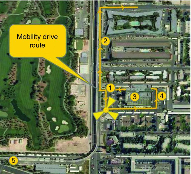
Figure 10.40 MIMO test route and stationary locations
Table 10.4 summarizes the stationary field results when MIMO was activated. The Virtual Antenna Mapping and MIMO with 64QAM feature set was activated with the S-CPICH set to 3 dB below the P-CPICH. The stationary throughput results show that when the SIR (Signal-to-interference ratio) dropped below 10 dB there is very little measurable gain from MIMO. The same device was used to perform the MIMO and dual-cell testing. Once the MIMO features were activated, no changes were made to the dual-carrier network configurations. The results show the relative comparison between HSPA+ Release 8 dual cell vs. Release 8 MIMO with 64QAM. An additional column is introduced to estimate the performance gain of MIMO as compared to a single carrier mode configuration.
Table 10.4 MIMO vs. DC performance measurements
| Stationary location | RSCP (dBm) | SIR (dB) | HSPA+ MIMO-42 (Mbps) | HSPA+ DC-42 (Mbps) | MIMO gain over single carrier (%) | Location relative to NodeB |
| 1 | −40 | 24 | 28 | 32 | 75 | LOS |
| 2 | −60 | 17 | 14 | 19 | 47 | LOS |
| 3 | −60 | 13 | 15 | 18 | 67 | NLOS |
| 4 | −70 | 10 | 11 | 15 | 47 | NLOS |
| 5 | −80 | 9 | 7 | 15 | −7 | NLOS |
HSPA+ MIMO operates in dual-stream and single-stream operation. The figure below shows the high correlation between device throughput and dual-stream operation along the drive route. As Figure 10.41 shows, the higher throughputs are achieved in areas where the device is requesting a high percentage of two transport blocks (dual stream). In other areas the UE only requests one transport block size (single stream) and the throughput rates drop accordingly.

Figure 10.41 Effect of MIMO dual stream on downlink throughput
MIMO is configured on the cell level, however it is recommend to be deployed on the market level because once a device is in an active data session and a P-CPICH from a non-MIMO cell falls into the active set the session will not be able to use MIMO again until the session is restarted in a MIMO configured cell. This can be observed toward the end of the drive on Figure 10.41. Note that mobility was maintained when there was a cell reselection to a non-MIMO cell, but in this particular vendor implementation, the UE will remain in single-carrier non-MIMO mode during the data session even if it re-enters MIMO coverage.
Figure 10.42 compares the performance of HSPA+ MIMO (single carrier) with Release 8 dual carrier, utilizing the same test device that was reconfigured from single-carrier 2 × 2 MIMO mode to dual-carrier mode. On average dual carrier outperforms MIMO by 60–70%, with relatively small performance differences in areas with good SIR. In this case, most of the drive was in fairly good radio conditions, so the throughput results may be slightly optimistic compared to more challenging mobility conditions. As expected, at the lower throughputs levels there was little to no gain in MIMO performance and the test device performance was similar to what you would expect from a device not configured with MIMO operating on a single HSPA+ 5 MHz carrier.
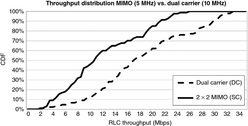
Figure 10.42 Throughput comparison, MIMO vs. dual carrier
By estimating the single carrier performance based on the dual cell performance that was collected in the field, MIMO shows an overall 15–25% improvement in spectral efficiency over Release 7 HSPA+ with 64QAM. These measured gains are consistent with other simulations and measurements [3].
10.5.4 Quality of Service (QoS)
The support of QoS is not a new item in HSPA+; however, normally the main differentiation factor has been the Maximum Bitrate (MBR) for the connection. In practice, QoS can provide an interesting feature toolset based on resource prioritization, to help the operator with items such as:
- subscriber differentiation
- application differentiation, and
- fair network use policies.
The use of resource prioritization is not relevant in networks with low traffic loads; however, as traffic increases and certain areas of the network get congested, 3GPP QoS can help deal with congestion in a cost efficient manner.
This section illustrates the behavior of utilizing quality of service prioritization in HSPA+ data networks, in particular the impact of assigning different data traffic priority levels to multiple users, under different loading conditions and traffic profiles.
The tests were performed in a live network configured with four different priority levels, which are configured following the guidelines summarized in Table 10.5: the users with the lowest priority (Priority 4) were set to receive approximately half of the throughput of users with Priority 3, one third of the throughput of users with Priority 2, and one fourth of the Priority 1 users.
Table 10.5 Summary of QoS test configuration and conditions
| Sector conditions | Medium-light load; tests during busy hour; RSCP = −93 dBm |
| Priority level of regular users | Priority 3 (2x) |
| Priority level of test users | Priority 1 (4x), Priority 2 (3x), and Priority 4 (1x) |
| Traffic profile | FTP DL, FTP UL, web browsing |
Two different sets of tests were executed, one with a single device sharing the sector with existing regular network users, and one in which three devices with a mix data profile were running simultaneously. The data profile consisted of multiple cycles of FTP upload and downloads of small and large files; and web download of multiple web pages (CNN, Expedia, Pandora, YouTube, Facebook, and others). Note that with this profile the devices often experience gaps in data transmission and reception due to the bursty nature of the web profile. The charts in Figure 10.43 illustrate the performance of the file downloads (a) and web browsing (b) for different priorities and load conditions.
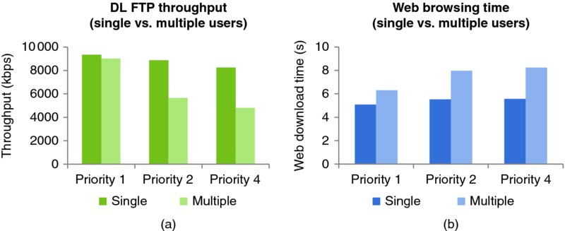
Figure 10.43 QoS Tests with initial settings: FTP (a) and web browsing (b)
The results show the impact of the different priority levels, which are only remarkable when the sector becomes loaded with the presence of other test devices. As can be noticed, the experienced throughputs do not necessarily follow the weights that were configured in the scheduler: even in the conditions with artificial load, there is not a significant differentiation between the Priority 2 and Priority 4 cases.
The following sets of tests illustrate the performance with more aggressive priority settings: Priority 1 (40x), Priority 2 (20x), Priority 3 (10x), and Priority 4 (1x). The objective of these settings was to heavily deprioritize the data transmission of Priority 4 users. Figure 10.44 shows the result of a single user test with different priority levels in a sector with medium–high load (50% TTI utilization), under good radio conditions. The default priority in the network was set to Priority 3.
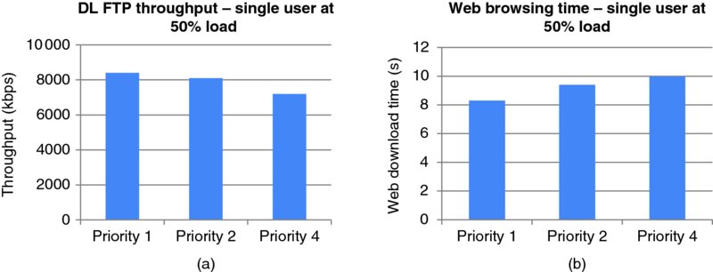
Figure 10.44 QoS tests with a single user in a loaded sector (a); evaluation of effect of different priorities (b)
As the tests results show, even with these aggressive settings the differentiation at the user experience level is barely noticeable; for example it takes only 20% more time for the Priority 4 user to download a web page as compared to the Priority 1 user. The differentiation only becomes clear in the case of overload, as Figure 10.45 illustrates.
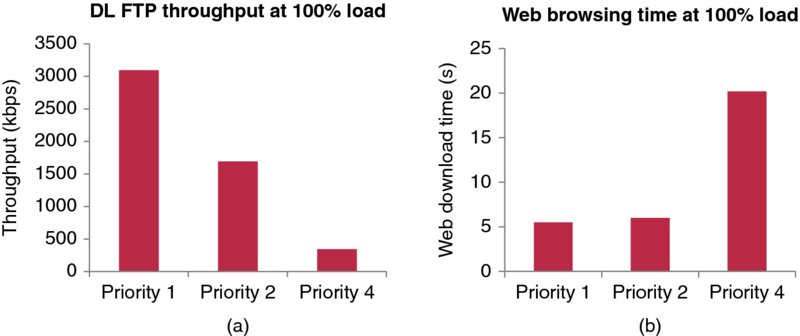
Figure 10.45 QoS results with aggressive settings on a sector with 100% load: FTP (a) and web performance (b)
The overload situation was created by having multiple users transmitting in the sector, achieving 100% TTI utilization. Only under these conditions is the differentiation clear, and it follows the guidelines set in the scheduler configuration. As such, this feature can be useful to manage extreme congestion situations when there is a clearly defined type of traffic that the operator needs to control. However it cannot be expected that it will provide a clear differentiation of the subscriber data experience across the network, since this greatly depends on the location of said subscriber.
10.6 Comparison of HSPA+ with LTE
The HSPA+ technology has continued to evolve over the years to provide potentially similar downlink air-interface speeds as LTE Release 8. In the USA, most LTE Release 8 deployments have initially been configured with 10 MHz of spectrum in the downlink. HSPA+ Release 8 dual cell uses the same bandwidth configuration of 10 MHz in the downlink. Both technologies also utilize 64QAM in the downlink, so if 2 × 2 MIMO was for some reason disabled on LTE, they would in theory provide very similar peak speed performance in excellent RF conditions. So the real difference in performance between the two systems should consist of the gains from 2 × 2 MIMO and any frequency domain scheduling gains that can be measured.
This section analyzes the performance of an experimental LTE system that is co-located with an existing HSPA+ network configured with dual cell. In order to perform the testing and compare the drive results a single drive was performed while collecting measurements on both HSPA+ dual cell and LTE with 2 × 2 MIMO activated. The HSPA+ network is a commercial network that has been in operation for a number of years, in which regular traffic load was present, while the LTE system was pre-commercial with no active LTE devices. HSPA+ dual cell and LTE Release 8 commercial dongles operating in the 2100 MHz band were utilized to perform this test. There is a one-to-one overlay in a relatively small geographic five-site cluster area. Both HSPA+ and LTE share the same antennas and utilize the same frequency band, so the coverage of the two systems should be very similar from a construction and deployment perspective. The drive route was chosen so that the measurements would be taken inside the overlay area. In an attempt to try and make the comparison between the two technologies as fair as possible, care was taken to only collect measurement data on the interior of the LTE coverage area: driving areas that were on the fringe of the LTE coverage where no inter-site interference was present would yield an overly optimistic LTE performance compared to an HSPA+ network with more neighbors and hence more inter-site interference.
Figure 10.46 shows the results of a mobility drive that compares HSPA+ dual cell to LTE that is using a 10 MHz downlink channel. The 2 × 2 LTE network achieved downlink peak speeds of nearly 68 Mbps, while during the same drive we measured a HSPA+ dual cell max speed of 32 Mbps.
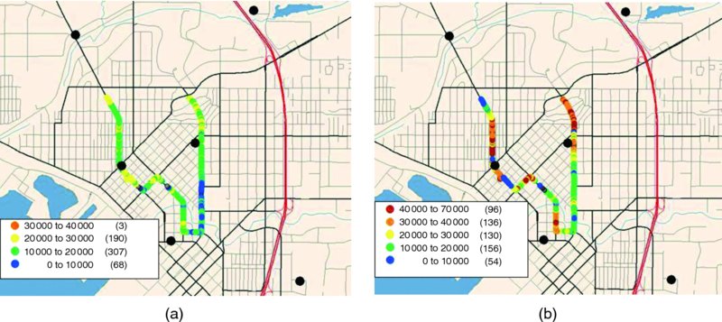
Figure 10.46 Mobility throughput (kbps): HSPA+ dual carrier (a); LTE 10 MHz (b)
Figure 10.47 illustrates the throughput distributions along the drives. The HSPA+ throughputs have been adjusted to account for non-scheduling periods (DTX rate) due to existing traffic, to facilitate the comparison between both technologies. It should be noted that the HSPA+ network also suffered from additional inter-cell interference due to the existing commercial traffic.
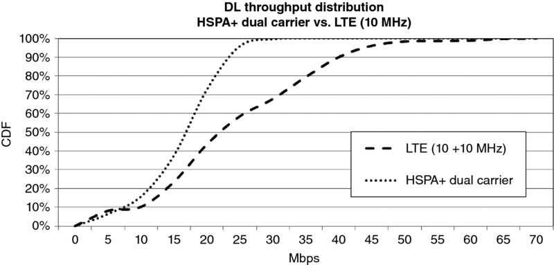
Figure 10.47 Comparison of HSPA+ vs. LTE (downlink). HSPA+ throughputs have been adjusted to account for non-scheduling periods (DTX) due to existing network traffic
On average, the LTE network provided around a 50% increase in downlink throughputs relative to HSPA+ dual carrier during the mobility drive while performing multiple FTPs in parallel. One interesting observation from the drive is that the performance of LTE was slightly worse than HSPA+ in very poor RF conditions, which was not expected. One reason could be that the LTE network had recently been deployed with little optimization. Also the LTE devices were relatively new and may not have had the same maturity as the HSPA+ devices. Regardless, even the measured difference was small and it is not expected that LTE will have a performance deficiency relative to HSPA+ as the technology is deployed in larger clusters.
Stationary results were also performed to compare the downlink throughputs, uplink throughputs, and latency. The latency results in Figure 10.48 show that there is a significant improvement in an LTE network due to the shorter TTI length (1 ms vs. 2 ms). It is interesting to note that the LTE latency shows a significantly better performance than HSPA+ in poor RF conditions. This may be explained by the fact that HSUPA uses 10-ms TTI in poor RF, which increases delay. On the other hand, 10-ms TTI may provide a better coverage than 1-ms TTI in LTE.
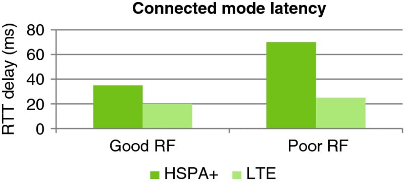
Figure 10.48 Latency comparison, HSPA+ vs. LTE
Stationary measurements are important because they give an indication of what a typical stationary user might experience on a wireless system, since often wireless customers are not necessarily mobile when using data services. Stationary measurements in good, medium, and poor RF conditions give an indication of how the air interface of a technology performs under realistic RF conditions that are geographically distributed over a wireless network coverage area.
The results in Table 10.6 show that the downlink throughputs of LTE Release 8 provide nearly twice the throughputs of HSPA+ dual cell. The uplink results of LTE are even more impressive; however, it should be noted that the HSPA+ network only used 5 MHz in the uplink direction. LTE uplink throughputs are between 3.5 to 7 times faster than HSPA+ which is consistent with 2x difference in bandwidth and the 2x potential increase due to higher modulation.
Overall, from a customer's perspective, HSPA+ dual cell provides downlink throughputs that are still competitive with a Release 8 LTE system operating with 10 MHz of bandwidth. However, LTE offers vastly superior uplink speeds that facilitate the adoption of uplink-heavy applications such as video conferencing.
10.7 Summary
This chapter has provided a detailed analysis of HSPA+ performance for downlink and uplink. Multiple HSPA+ features have been discussed, including Release 8 dual cell, MIMO, and advanced receivers. During the analysis, it has been shown how different vendor implementations can have a significant impact on data performance, mostly driven by the implementation of their specific link adaptation methods.
Table 10.7 summarizes the expected data rates in commercial networks under various radio conditions; it also provides the performance of an equivalent LTE network that was unloaded at the time of the tests, for comparison purposes.
Table 10.6 Summary of stationary tests performance, DC-HSPA vs. LTE
| Good signal strength (Mbps) RSCP: −65 dBm, Ec/No: −3 dB RSRP: −80 dBm, RSRQ: −5 dB | Typical signal strength (Mbps) RSCP: −90 dBm, Ec/No: −5 dB RSRP: −94 dBm, RSRQ: −7 dB | Poor signal strength (Mbps) RSCP: −102 dBm, Ec/No: −9 dB RSRP: −116 dBm, RSRQ: −8 dB | |
| HSPA+ DL | 31 | 18 | 5 |
| LTE DL | 55 | 35 | 9 |
| HSPA+ UL | 2.7 | 2.1 | 1.4 |
| LTE UL | 13 | 14 | 5 |
Table 10.7 Overall performance summary: stationary throughput tests
| Good signal strength (Mbps) | Typical signal strength (Mbps) | Poor signal strength (Mbps) | |
| HSDPA single carrier | 13.5 | 9 | 2.5 |
| HSDPA dual carrier | 28 | 18 | 5 |
| HSUPA | 4.1 | 2.1 | 1.4 |
| LTE 10 MHz downlink | 55 | 35 | 9 |
| LTE 10 MHz uplink | 13 | 14 | 5 |
In terms of latency, the results have shown that, depending on the radio conditions, HSPA+ networks will offer typical round-trip latency values between 25 and 70 ms.
Overall, the HSPA+ technology offers a compelling data performance even when compared to LTE networks – furthermore, as will be discussed in more detail in Chapter 13, the quality of experience offered to the end customer is still competitive with networks offering higher nominal speeds.
Notes
References
- 3GPP TS 25.214: Physical Layer Procedures (FDD), Release 8.
- 3GPP TS 25.213: Spreading and Modulation, Release 8.
- “MIMO in HSPA; the Real-World Impact”, GSMA, July 2011.