
12
Radio Network Optimization
Pablo Tapia and Carl Williams
12.1 Introduction
To ensure an optimum operation of the HSPA+ technology the operator has to make a multitude of decisions when planning and optimizing the network, considering multiple components: from the device to the network and up to the application servers. In a HSPA+ system there are four main areas that the operator needs to address in order to achieve the desired service performance:
- Radio network planning, such as the location of cell sites, orientation of antennas, transmit power adjustments, and radio network capacity adjustments.
- Transport and core network planning, which will determine the latency and capacity of the backhaul and interconnection links, the location of the core network nodes, and the corresponding core network capacity adjustments.
- Terminal devices. The devices are a major component of the experience of the customer, and care should be taken on the selection of the right hardware components such as CPU and memory, the optimization of transceiver and radio modem, selection and adaptation of the OS, and development and adjustment of apps.
- Soft parameters, which control the adjustment of radio and core functionality such as resource allocation, scheduling, and mobility management procedures.
When planning and optimizing the network, there will often be a tradeoff between quality, capacity, and cost. In some cases, if certain key guidelines are followed, tradeoffs are not necessary and the operator will achieve the maximum potential of the technology with a minimum cost. This chapter will provide the operator with important HSPA+ guidelines, as well as explain some of the tradeoffs that are possible when optimizing the HSPA+ technology from a radio network standpoint; planning and optimization aspects for other parts of the system will be covered in other chapters: Chapter 11 (Network Planning) has already discussed strategies to deploy the radio, transport, and core, while specific device optimization will be covered in detail in Chapters 13 and 14.
The latter part of the chapter is dedicated to engineering tools. In the last few years, new tools have been developed that can greatly help engineers with their network optimization and maintenance tasks, especially in today's situation, in which engineers need to deal with increasingly growing traffic levels and deal with multiple technologies simultaneously. The chapter will describe some of the new tools that are available for HSPA+, illustrating with real network examples how an operator can make use of them to optimize their network capacity and performance.
12.2 Optimization of the Radio Access Network Parameters
The principal bottleneck of HSPA+ typically lies on the radio interface. The wireless link is not reliable by nature, with multiple factors affecting its performance: pathloss, shadow and fast fading, load and interference, user mobility, and so on. While the HSPA+ system has special mechanisms to overcome many of these challenges, such as link adaptation and power control, they require special adaptation to the network conditions to operate at an optimum point. For example, the handover triggers in a highway cell need to be set to enable a fast execution of the cell change procedure, otherwise the call may drag too long and result in a drop; on the other hand, these triggers may need to be set more conservatively in low mobility areas with non-dominant pilots, to avoid continuous ping-pong effects that also degrade the service performance.
In today's fast changing networks, radio optimization must be considered a continuous activity: once the network is deployed, it will require constant tuning since traffic patterns change with time, as load increases and new mobile phone applications put the network to the test. Some useful guidelines to tackle network optimization are:
- Recognize when the problem is due to improper planning: trying to compensate for a planning problem through network optimization is sometimes possible, but it will result in a suboptimum performance and capacity situation; whenever possible, planning problems should be identified and tackled before optimization.
- Optimize key traffic areas first: it is impossible to achieve a perfect optimization of the whole network, so where the majority of traffic is should be taken into consideration.
- Don't rely solely on network KPIs: sometimes network KPIs are hard to interpret, especially those related to data services. Driving the network gives the engineer a totally different perspective of what's happening in certain areas.
To support the optimization activity it is recommended to drive test the areas with a certain frequency, since this is the best way to figure out problems in the radio layer. Alternatively, as the network becomes more mature, the operator could use other tools to minimize drive testing, as will be discussed later in Sections 12.3.1 and 12.3.2.
There are multiple functional areas that can be optimized in HSPA+, including antenna parameters, channel powers, handover parameters, and neighbor lists, among others. This section will provide an overview of possible optimization actions on each one of these areas; it also provides a detailed analysis on causes and solutions to optimize uplink noise rise, one of the major capacity problems on HSPA+ networks with high smartphone traffic penetration.
12.2.1 Optimization of Antenna Parameters
Once deployed, HSPA+ networks will be in a state of continuous change: cell breathing due to increased traffic, creation of new hotspot areas, introduction of new sites, and so on; when necessary, antenna parameters should be adjusted to improve network capacity or performance. Normally, the adjustment of the antennas post-launch will focus exclusively on tilts: antenna height changes are very rare, and azimuth modifications have very little impact unless a significant rotation angle is required. Since the adjustments of the antenna tilts can be quite frequent, it is recommended to use Remote Electrical Tilts (RET) capable antennas as much as possible to avoid visiting the site location, which is normally an expensive and time consuming thing to do.
As with other wireless networks, in HSPA+ the throughput and capacity are heavily tied to interference. The main source of interference in HSPA+ is the power coming from other sectors, which is especially harmful in areas where there is no clear dominant pilot (pilot pollution). In addition to interference, pilot polluted areas are prone to “ping-pong” effects during HS cell changes, which also result in lower throughputs and an overall poor service experience.
Figure 12.1 illustrates the interference (left) and corresponding throughput (right) of a single carrier HSPA+ network. As can be observed, the areas with higher interference – darkspots corresponding to low Energy over Noise and Interference ratio (Ec/No) – is where the HSPA+ throughput becomes lower (mid-gray colors on the right figure).
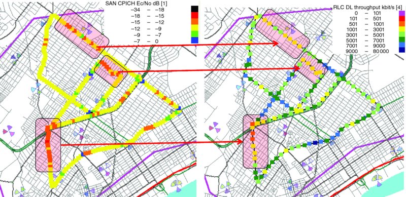
Figure 12.1 Correlation between interference (indicated by Ec/No) and throughput in a live network
To mitigate these spots, the antenna tilts in the cluster were adjusted to try and ensure proper pilot dominance. The key metrics to monitor in this case are:
- The best serving cell at each location, to ensure that each area is being served by the nearest sector, and that proper cell boundaries are attained.
- Geolocated traffic and Received Signal Code Power (RSCP) samples, to avoid degrading the customers with lower signal strength.
- Signal quality metrics, such as Ec/No and Channel Quality Indicator (CQI), which will provide an indication of the interference situation in the cluster.
- Throughput, captured by a drive test tool.
- IRAT handovers and 2G traffic, to ensure that the optimization is not achieved by pushing traffic to the underlying GSM system.
A good method to analyze this exercise is to display the best server plots: Figure 12.2 illustrates the best server plot before and after the antenna adjustment. As the figure shows, while not perfect, the optimization exercise improved the pilot dominance in the border areas. Perfect cell boundaries are hard to achieve in practice, especially considering urban canyons, hilly terrains, and so on.
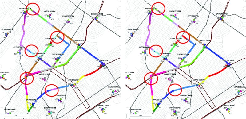
Figure 12.2 Best server plot, before and after antenna optimization
In this particular example, the average CQI improved by 1.5 dB and the average throughput in the area increased by 10%, as a result of the better interference situation. The antenna adjustments included uptilts and downtilts, and in one particular case one of the sectors was shut down since all it was doing was generating harmful interference. It is not uncommon to find useless sectors in the network, especially when the HSPA+ sectors are co-located with existing GSM sites that may have been deployed for capacity reasons.
Figure 12.3 provides an antenna optimization example using geolocated data. Figure 12.3a displays the sector traffic samples before the optimization, with darker spots indicating areas with high interference (low Ec/No); as the plot shows, there are a number of traffic samples being served quite far away from the sector, in fact getting into the footprint of sectors that are two tiers away – this is known as an overshooting situation. Figure 12.3b shows the traffic after the sector has been optimized (in this case through downtilt), in which the samples are mostly contained within the cell footprint. Geolocation tools will be discussed in more detail in Section 12.3.
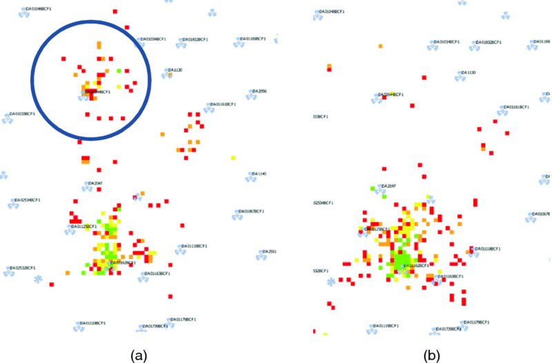
Figure 12.3 Analysis of geolocated samples from one sector before (a) and after (b) tilt optimization
As discussed in Chapter 11, it is important to avoid excessive antenna downtilts. Downtilting is often abused in UMTS networks as the only method to achieve interference containment, however doing it in excess can create significant coverage issues, especially in sectors with low antenna height. Cell power adjustments can be used as a complement to antenna tilts to achieve a good delimitation of cell boundaries.
When downtilting or reducing the CPICH it is possible that the main KPIs show a performance improvement, however the sector may be losing coverage. It is important to monitor the traffic and IRAT levels to prevent these situations, and if possible validate the new coverage footprint with drive test data or with the help of geolocation tools.
12.2.2 Optimization of Power Parameters
One of the key parameter sets that need to be tuned in a HSPA+ network is the power assigned to the different physical channels. Typically in UMTS networks the operator can control the power level assigned to the following channels:
- Common Pilot Channel (CPICH)
- Downlink Common Control Channel (CCCH): Broadcast Channel (BCH), Acquisition Indicator Channel (AICH), Paging Channel (PCH), Primary Synchronization Channel (P-SCH), Secondary Synchronization Channel (S-SCH), Paging Indicator Channel (PICH), and Forward Access Channel (FACH).
- Release 99 (R99) Dedicated Data Channels.
- R99 Voice Channels.
- HSDPA Channels: High Speed Shared Control Channel (HS-SCCH) and High Speed Downlink Shared Channel (HS-DSCH).
12.2.2.1 Adjustment of Common Control Channels
The power allocation of the control channels needs to be done carefully since it will have implications for both coverage and capacity planning. The total amount of power available in the Power Amplifier (PA) is limited and the operator needs to strike the right balance between power allocated to the control and data channels.
A general guideline to follow is to assign about 10% of the total power to the pilot, and 15% to the remaining control channels (since FACH is not always transmitting, the typical common channel power consumption would be in the order of 5%), thus leaving between 75 and 85% of the total PA for data channels. When more power is used for the control channels, the coverage of the cell may be extended, or it may improve the connection reliability, however the capacity of both voice and data will be reduced in that sector. The golden rule in WCDMA optimization is to always try to provide the least possible power that provides a good service experience: when too much extra power is used when not needed, it will create unnecessary interference in the network that will degrade the performance in the long run.
The power assigned to the CPICH channel and the CCCH have a direct impact on the coverage of the cell, since they control the power boundary of the cell and the power allocated to the access channels. The power assigned to the data channels also has an impact on the offered quality of the service: for example, if the operator limits the power on the voice channel, it may suffer higher packet losses (BLER), which degrades the MOS score, and may result in a dropped call.
The default values provided by infrastructure vendors are sometimes not optimum for the needs of the operator. In some cases, the values are set too conservatively to meet certain contractual KPIs, at the expense of network capacity. It is therefore recommended to review and tune the power parameters based on the specific situation of the operator. Table 12.1 provides some parameter ranges for the most relevant CCCH. With the introduction of Self Organizing Networks (SON) tools, it is possible to adjust these settings for each particular cell, unlike the typical situation in which these are configured equally across the whole network. SON tools will be discussed later in Section 12.3.3.
Table 12.1 Typical parameter ranges for CCCH power settings
| Typical values | |||
| Network | (in reference to | ||
| Channel | Description | impact | CPICH) |
| CPICH (common pilot) | Transmits the pilot of the cell | Accessibility Retainability | 0 |
| AICH (acquisition indicator) | Indicates a data channel to be used by the UE | Accessibility | −7 to −8 dB |
| BCH (broadcast) | Provides information about the network and cell | Accessibility | −3 to −5 dB |
| PCH (paging) | Alerts the UE of incoming communication | Accessibility | −0.5 to 0 dB |
| P-SCH (primary synchronization) | Enables UE synchronization with the network | Accessibility Retainability | −3 to −1.5 dB |
| S-SCH (secondary synchronization) | Enables UE synchronization with the network | Accessibility Retainability | −4 to −3 dB |
| FACH (forward access) | Transport for small amounts of user plane data | Accessibility Retainability | 0 to +1.5 dB |
| PICH (paging indicator) | Provides information about the transmission of the PCH | Accessibility | −8 dB |
The following example shows a case in which the network CCCH has been optimized, adjusting the default power values to a lower level while keeping the same network performance. The following changes were implemented:
- BCH: from −3.1 dB to −5 dB
- AICH: from −7 dB to −8 dB
- P-SCH: from −1.8 dB to −3 dB
- PICH: from −7 dB to −8 dB.
Figure 12.4 summarizes the impact on the cluster, both on capacity (Tx power, on the left), as well as on the main network quality metrics (right chart).
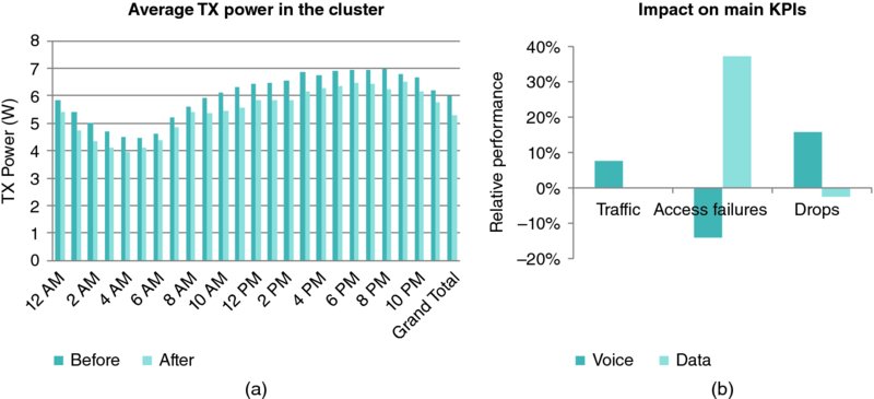
Figure 12.4 Average power reduction in the cluster (a) and main network KPIs (b)
This resulted in an average power reduction of 12% in the cluster, with a higher reduction on the top loaded sectors in the area, thus providing an important capacity saving in the network. The main KPIs in the network were improved, or didn't suffer, with the exception of the voice access failures, which were slightly degraded.
12.2.2.2 Adjustment of Pilot Power
The selection of pilot power is normally one of the first tasks to be done when preparing the network planning. The power of the pilot is normally chosen to be equal in all sectors of the same cluster, and a small percentage of the maximum desired carrier power – typically 10%. Keeping homogeneous pilot power simplifies the network deployment; however, in mature networks it may be a good idea to adjust the pilot powers depending on traffic load and coverage needs of each individual sector. The best way to achieve this in practice is with the help of SON tools, which will be discussed later on Section 12.3.3.
While in the initial UMTS days the power amplifiers typically had a maximum power of 20 W, today Power Amplifier (PA) technology has evolved and existing units can transmit 80 W or more. This power can be split into several carriers, thus providing the possibility of adding more sector capacity with a single piece of hardware – provided the operator has the spectrum resources to allow for an expansion.
While it is often tempting to make use of all the available power resources in the PA, the operator needs to consider future possible capacity upgrades before deciding how much power to allocate to each carrier. Furthermore, in the case of UMTS, having more power does not provide any additional advantages beyond a certain point, once the basic coverage is ensured in the area.
The following example illustrates the case of a real network that was originally configured to operate at 40 W per carrier, and was converted to transmit with a maximum power of 20 W in all sectors. The trial area included a mixed urban and suburban environment with an average intersite distance of 1.2 km; the average RSCP reported by the network was −92 dBm, which may be considered as coverage challenged area. The trial area and RSCP distributions can be observed in Figure 12.5.

Figure 12.5 Trial area (a) and RSCP distribution (b)
In this exercise, both the maximum transmit power of the sector and the pilots were modified. Each of the pilots was adjusted depending on its specific traffic and coverage needs. Some antenna tilts were also adjusted to compensate for power losses, if necessary. At the end of the exercise, the pilots in the area were reduced by an average of 1.8 dB, and the average transmit powers were reduced by 2.25 dB. As a consequence of the lower power used, the drive test results indicated an improvement of Ec/No of 1.5 dB in the area. The lower powers did not result in traffic loss, neither for voice or data, as can be observed in the data traffic volume trend in Figure 12.6b.
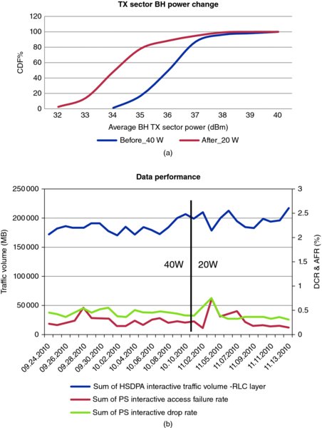
Figure 12.6 Average transmit power (a) and data KPIs (b), before and after the change
As Figure 12.6 illustrates, the power reduction did not have a negative impact on network KPIs. A small throughput reduction was observed in the cluster (5%) due to the lower power available. The rest of the KPIs were maintained, with some improvement observed on IRAT performance, probably due to the mentioned Ec/No improvement. A similar exercise performed in an urban environment with better coverage revealed further capacity gains, with 3.5 dB reduction in overall transmit power, and no impact on network KPIs.
In summary, the adjustment of the pilot power can be an effective tool to optimize the interference situation in the network. The operator needs to decide what the right tradeoff is between offered capacity, throughput, and cost, and configure the pilot power accordingly.
12.2.2.3 Adjustment of Voice Channel Power
In HSPA+ networks the spectrum resources are shared between voice and data channels, in addition to the control channels previously discussed. While voice payload is typically very small when compared to data, the dedicated nature of the voice channel allows it to utilize a fair amount of power resources in the system, therefore increasing the overall noise in the network and contributing to data congestion in hotspot areas. Furthermore, HSPA+ networks are typically configured to assign a higher priority to voice channel allocation over data channels, which will result in an overall reduction of data capacity in loaded sectors. This is more of a concern on downlink traffic, given that in today's networks data traffic is heavily asymmetric, with a typical ratio of 7:1 in downlink vs. uplink data payload.
As Figure 12.7 shows, it is not unusual to find heavily loaded sites dominated by voice load rather than data load. In this particular example, almost half of the available power is consumed by voice.
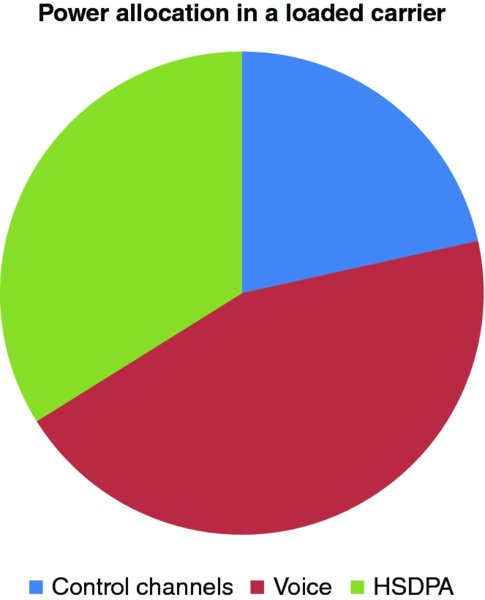
Figure 12.7 Channel power breakdown in a loaded carrier
One option to minimize the impact of downlink voice channels on data performance is to optimize the power ranges allowed for the voice channel. This is usually configured through a parameter that indicates the maximum power allowed per radio link. Given that the base stations are configured to transmit with a 20 dB dynamic range, setting the power per radio link too high may force them to transmit at a higher power than required in areas with good radio conditions.
A good method to determine whether the power per radio link is too conservative is to extract the statistics of the downlink power distribution. Figure 12.8 illustrates a sector in which the power allocated to the voice channel is constrained by the dynamic range. In this particular case, the maximum power per radio link was set to −15 dBm.
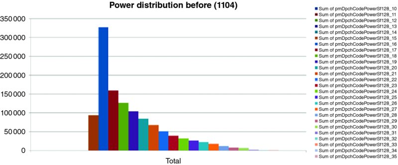
Figure 12.8 Suboptimal voice power distribution in a sector (leftmost bins correspond to lower transmit power)
Figure 12.9 show the effect of the adjustment of the voice link channel power, from −15 to −18 dB. As can be observed on the voice channel power distribution (left chart) the network is operating in a more optimum manner after the adjustment, which also results in overall capacity savings. The trend on Figure 12.9 (right) shows that this optimization resulted in about 1 dB average power reduction per link.
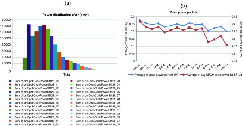
Figure 12.9 Results from optimization of voice channel power
12.2.3 Neighbor List Optimization
The optimization of UMTS neighbor list is one of the most frequent network maintenance tasks that field engineers need to tackle. The intra-frequency, inter-frequency, and IRAT neighbor lists should be continuously modified to cope with changes in traffic and to accommodate new sites that may be coming on air. If this task is not diligently performed on a regular basis, the network performance will be impacted via an increase of drops, typically revealed as drops due to missing neighbors, or UL synchronization. In some extreme cases, the drops due to missing neighbors can account for up to 20% of the total number of drops in cluster.
Typically the engineers will have some computer tool available to facilitate the configuration of neighbors. These tools range from basic planning tools, in which the neighbors are configured based on RF distance, to Self-Organizing Networks (SON) tools that will automatically configure the neighbors on a daily basis. SON tools will be discussed in more detail in Section 12.3.3.
Initially, the neighbor lists should be configured based on planning information, and typically include at least the first and second tier neighbors. Neighbor lists don't need to be reciprocal, but it's a good idea to enforce reciprocity between different carriers of the same site to facilitate traffic load balancing. Defining the right 2G neighbors is also very important, especially in the case of rural sites.
Once the network has a sufficient amount of traffic, the neighbor lists should be maintained based on network statistics, such as handover attempts, success and failures, drop call rate, and so on. It is a good idea to activate detected set measurement, and make use of these reports to identify missing neighbors. It is also important to keep the neighbor lists well pruned, and remove unused neighbors to leave room for possible new cells showing up in the future. Also, if an extended neighbor list is in use – that is, System Information Block (SIB) 11bis is broadcast – it is important to arrange these lists to keep high priority neighbors in SIB11 and lower priority neighbors in SIB11bis. Note that SIB11bis can only be used by Release 6 compliant terminals.
The engineer should also be on the lookout for possible handover problems due to wrong neighbor selection, as well as overshooting sectors, which will tend to generate handovers to an excessive amount of sectors. The incorrect neighbor problem can normally be fixed with scrambling code disambiguation, or ultimately with re-assignment of new scrambling codes for those conflicting sectors. The overshooting sector problem should be tackled with proper RF optimization.
Figure 12.10 shows an example of an RNC where a neighbor optimization exercise was run using a SON tool: once the optimization task started, the number of drops due to missing neighbors in the area was significantly decreased.
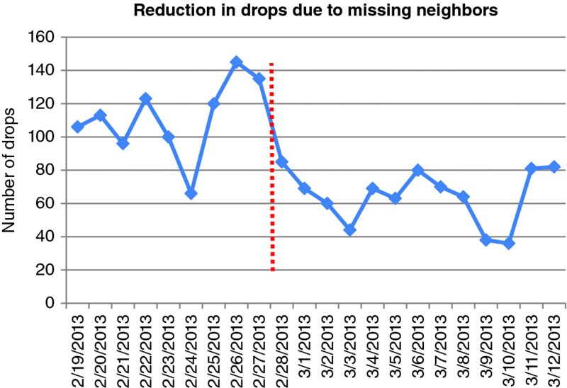
Figure 12.10 Neighbor optimization exercise in one RNC
In general, it is hard to eliminate all missing neighbors due to constraints on neighbor list sizes. The different neighbor lists (intra-frequency, inter-frequency, and inter-RAT) all have size limitations, as well as the overall combined list. Configuring more neighbors than permitted can create serious problems in the sector, derived from SIB11 congestion, which in extreme cases can put the site off service and will require a site reset to be fixed. For this reason it is a good idea to maintain a pruned list size, eliminating the neighbors that are not strictly required as previously discussed.
Some infrastructure vendors provide special reporting of the detected set neighbors, which are neighbors not contained in the neighbor list that are properly decoded by the UE using soft handover event triggers. These special reports provide aggregated information containing the RSCP and Ec/No value of the detected scrambling code, and can be useful to identify missing neighbors in live networks.
12.2.4 HS Cell Change Optimization
The mobility performance in HSPA+ presents significant challenges due to the nature of HS cell change procedure, which is significantly different from the handover method of the original UMTS dedicated channels. The R99 UMTS systems included soft handover mechanisms to avoid the harmful effects from adjacent cell interference that are inherent in systems with a single frequency reuse: the user plane transmission was never interrupted, and links from multiple sectors could be combined to improve the performance at the cell edge.
In the case of HSDPA, and to a certain extent of HSUPA, the transition between sectors can result in a reduction of user throughput due to the interference levels endured at the cell boundary: since the device is only transmitting and receiving data from one sector at a time, the new target sector will become a source of interference until the cell change procedure has been completed. In addition to this interference problem, it is not uncommon to observe “ping-pong” effects, by which the UE bounces back and forth between two cells that have similar power levels, which sometimes further degrade the offered HSPA throughput.
More recently, the HSDPA performance at the cell edge has been significantly improved thanks to the wide adoption of Type 2i and 3i receivers which are able to cancel the strongest sources of interference in the HS-DSCH channel. Advanced receivers were presented in Chapter 8, and practical performance aspects were discussed in Chapter 10.
While HSUPA was designed to use Soft Handover (SHO), the cell change procedure suffers from practical limitations that impact its performance. For example, some infrastructure vendors limit the SHO utilization to the control plane alone to limit excessive baseband consumption for users in border areas. Furthermore, the HSUPA cell changes will follow the change of serving cell decided on downlink, and thus will also be impacted by ping-pong effects in the HSDPA cell change.
The HS cell change procedure can be triggered by an explicit event (1D), by which the UE notifies the network of a more suitable serving cell, or implicitly following a soft handover event (1A–1C). The event triggers can be based on RSCP or Ec/No, or both, depending on vendor implementation. Table 12.2 summarizes the relevant UE events that can trigger a cell change procedure.
Table 12.2 UE Events that can trigger a HS cell change
| Event | Impact |
| 1A | SHO radio link addition |
| 1B | SHO radio link removal |
| 1C | SHO radio link replacement |
| 1D | Change of best cell |
These events are configured on the network side, and are typically defined with a level threshold and a time to trigger. Very short trigger times can lead to an excessive number of cell changes and frequent ping-pong, while very long times can result in decreased quality (CQI) due to a longer exposure to interference. The metric used to trigger the event is also relevant: for example, events triggered based on Ec/No can result in higher fluctuations in the case of HSDPA data.
It is important to realize that macro level network KPIs can sometimes mask some of these problems that occur only in specific areas, such as cell boundaries. Customers that are located in cell boundary areas may be experiencing a consistent poor data experience, but these problems will go unnoticed because these stats will be combined with the overall sector KPIs. Therefore, to tune the performance at these locations the best course of action is to rely on drive test exercises, or alternatively on geo-located KPIs. Section 12.3.2 discusses a set of tools that can be very useful to troubleshoot and optimize this type of problem.
In the following example we analyze the performance of a cluster that presented a high number of ping-pong effects, which resulted in poor data performance in those particular locations. The performance degradation could be noticed even during stationary conditions when located in the cell boundary areas.
The objective of the exercise was to reduce the amount of unnecessary cell changes, with the ultimate goal to improve the throughput in those challenging areas. Table 12.3 summarizes the original parameter settings controlling the HS cell change, as well as the optimized settings adopted during the trial.
Table 12.3 Results from HS cell optimization exercise
| Parameters | Baseline | Optimized | Unit |
| Addition window | 1.5 | 0 | dB |
| Drop window | 3.5 | 6 | dB |
| Replacement window | 1.5 | 3 | dB |
| Addition time | 320 | 640 | ms |
| Drop time | 640 | 1280 | ms |
| Replacement time | 320 | 1280 | ms |
| HSDPA CPICH Ec/No threshold | −5 | −9 | dB |
Figure 12.11a illustrates the trial area, in which the sectors with higher data loads are indicated with a darker color. It shows the stationary test locations, as well as the selected test drive route, which was chosen to go through equal power boundary areas where there was no clear cell dominance. As discussed earlier, these are the most challenging conditions for HSDPA traffic channels. The Figure 12.11b shows the throughput distribution along the drive route, with baseline (light gray) and new parameters (dark gray).
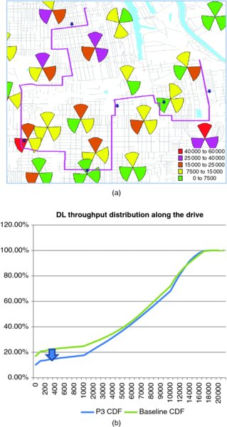
Figure 12.11 HS cell change optimization area (a) and throughput distribution (b)
As the throughput distribution in Figure 12.11b shows, the performance for the customers in the worse performing areas was significantly improved with the new parameters. For an equal percentile (20% on the chart), user throughputs increased from 100 kbps to 1.5 Mbps. As Figure 12.12 illustrates, the tests performed in stationary locations also showed improved performance for users in poor locations, both for simple download as well as web browsing performance – on the other hand, users in good RF locations suffered a slight reduction in uplink throughput.
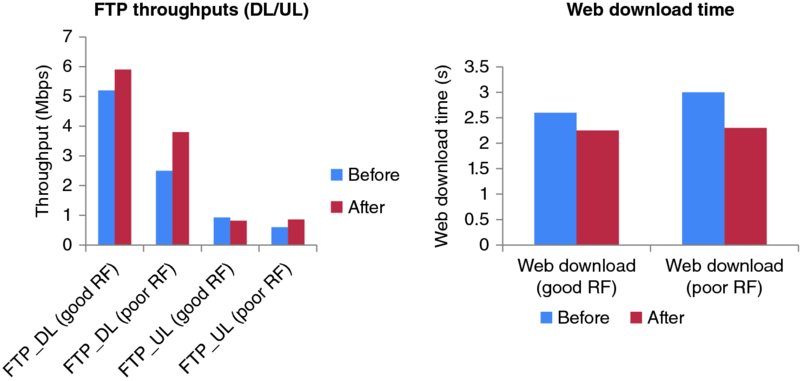
Figure 12.12 User experience improvement with new settings
Other benefits from these settings included up to a 30% reduction in HS cell changes, reduction in SHO events and SHO overhead, and reduction of radio bearer reconfigurations as well as R99 traffic.
It should be noted that these results may not be applicable to every network, since the settings depend heavily on the underlying RF design, as well as the characteristics of the cluster. For example, these settings are not recommended for areas with high traffic mobility.
12.2.5 IRAT Handover Optimization
When UMTS networks were originally introduced, the use of Inter Radio Access Technology (IRAT) handovers was a simple and reliable mechanism to ensure service continuity in areas with discontinuous 3G coverage. On the other hand, IRAT handovers introduce an additional point of failure in the system, and result in a poorer customer experience as well as reduced system capacity since the underlying GSM system is not well suited to transfer high speed data connections.
The use of IRAT handovers can often mask underlying RF performance issues in the network that are not reflected in the typical network indicators: users in areas with poor performance will handover to GSM instead of dropping in UMTS – they may later on drop in GSM as well, but this drop is not considered in the UMTS optimization and this results in a poorly optimized network exercise.
Frequent IRAT also increases the probability of missing paging. Call alerts may be missed when the devices are in the middle of a transition between technologies and the location area update has not been completed. Although this problem can be mitigated with MSS paging coordination, this is a complicated problem to troubleshoot, since there are no counters that keep track of these events.
In general, as networks mature and a sufficient penetration of 3G sites is achieved, operators should try and minimize the utilization of IRAT handovers whenever possible. It is recommended to try and disable IRAT in areas with 1 : 1 overlay; if there is not 100% overlay, the default parameters can be adjusted with more aggressive settings at the expense of a higher drop rate in UMTS – however this increase is often compensated with a drop reduction in the underlying GSM layer.
Figure 12.13 illustrates an example in which the voice IRAT thresholds were reduced to a very aggressive setting (RSCP level of −120 dBm, Ec/No of −15 dB). Note that these values were used for testing purposes and may not necessarily be appropriate for a widespread use in commercial networks.
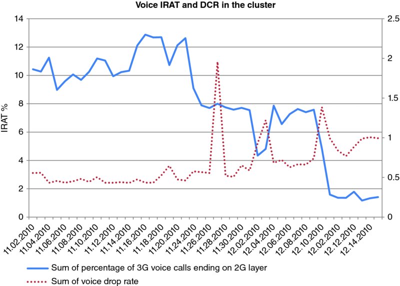
Figure 12.13 Optimization of voice IRAT settings
The test cluster was the same one referenced in Section 12.2.2.2, where there was approximately a 70% overlay between UMTS and GSM sites. In the example, the IRAT ratio was reduced from an original 10%, down to a level close to 1%. The 3G dropped call rate in the area subsequently increased from 0.5 to 1%. On the other hand, the 2G drop rate improved, because there were not so many rescue calls going down to the GSM layer. At the end of the day, each operator will need to decide their own specific tradeoffs between 3G traffic share and 2G/3G traffic quality.
In the case of HSDPA data, the service is more forgiving to poor radio conditions and thus permits even more aggressive settings to retain the traffic on the HS channel. There are two sets of parameters controlling this, the PS IRAT parameters as well as the parameters controlling the transition from HS to DCH. Figure 12.14 shows the case of a network in which these settings have been aggressively adjusted:
- HS to DCH transitions due to poor quality OFF.
- Ec/No service offset for Event 2D (used by compressed mode) from −1 dB to −3 dB.
- RSCP service offset for Event 2D (used by compressed mode) from −6 dB to 0 dB.
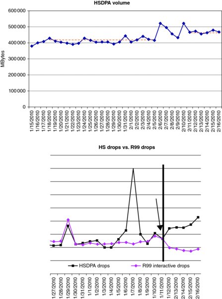
Figure 12.14 Optimization of PS traffic retention in the HSPA layer
By adjusting these settings the users will stay longer in HSDPA, thus avoiding unnecessary transitions to R99 – which is a less efficient transport – or ultimately 2G. Figure 12.14 shows the impact of the change on the overall HSDPA traffic volume (left), which increased by 12%; the chart on the right shows the impact of the change on PS drops. The overall packet drop rate remains stable, although there was an increase in HSDPA drops that was offseted by a reduction in R99 drops.
Nowadays, many operators have completely removed IRATs for data and some operators also for voice, which has typically resulted in better KPIs, assuming that the UMTS coverage is sufficiently good. If IRAT is used for data, then it is normally triggered only by RSCP and not by Ec/No.
12.2.6 Optimization of Radio State Transitions
Section 4.10 in Chapter 4, and Section 10.3 in Chapter 10 discussed how the delay in the radio state transitions has an important impact on the HSPA+ latency, and therefore on the final data service experienced by the customer. While packets on the DCH state enjoy a fast transfer speed and a protocol architecture that minimizes latency, those packets transmitted over the FACH channel will be transferred at a very slow speed. Even worse is the case where the device is in a dormancy state, either IDLE or PCH, in which case there is an additional delay to set up the corresponding channel.
The following diagram (Figure 12.15a) illustrates the typical RRC state transitions in today's networks. The diagram does not include the IDLE state, since nowadays it is widely accepted that the default dormancy state should be Cell_PCH (either Cell_PCH or URA_PCH). This is due to the fact that the transition from Cell_PCH is much faster than from IDLE, and involves a significantly lower amount of signaling messages, as illustrated in Figure 12.15b.
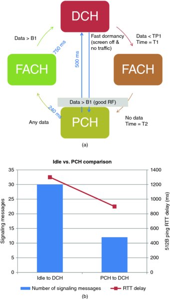
Figure 12.15 Illustration of RAN state transitions for HSPA (a) and comparison between idle and PCH performance (b)
When the UE is in the PCH state, a new data packet that needs to be transmitted can either be sent via DCH – if the direct transition feature is activated and certain conditions are met – or via FACH. To trigger a direct DCH transition the data volume should be larger than a certain threshold (B1, on the diagram); in certain implementations there is also a quality criterion, by which the direct transition is only triggered if the Ec/No is better than a certain threshold. Figure 12.16 illustrates the result from a trial network in which different quality thresholds were tried. As the threshold is relaxed, the amount of direct transitions increase, but there's also an increase in upswitch failures.
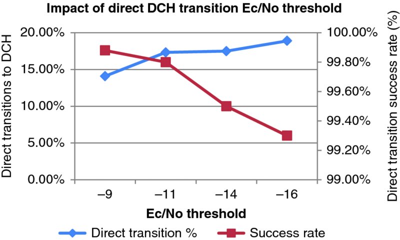
Figure 12.16 Impact of different Ec/No thresholds on the PCH to DCH direct transition (buffer size = 512 B)
When the UE is in FACH state, it will transmit at a very low bitrate, typically 32 kbps. If the application data volume increases beyond a threshold B1, a transition to DCH will be triggered; this promotion time is quite slow and can take around 750 ms, so in general the operator should avoid entertaining continuous FACH<->DCH transitions. When there is no data to be transmitted, the UE will fall back to PCH (or IDLE) state after an inactivity time (T2).
The DCH state is the fastest state, where the user can enjoy minimum latency (as low as 25 ms) and high-speed data transfer. The UE will fall back from this state into FACH state in case the transmission speed falls below the TP1 threshold for a certain amount of time (T1). There is also a possible DCH to PCH direct transition for mobiles that implement the Release 8 fast dormancy feature that is described in Chapter 4. This is typically triggered when there is no additional data to be transmitted, and the phone screen is off.
The configuration of the HSPA+ radio states parameters is a complex task as it affects many different factors. For example, a large T1 timer will have a good effect on user experience, but may create capacity issues in the cell. Similarly, a low B1 buffer to transition to DCH would reduce latency, but can degrade some network KPIs. The following summarizes the impact of these parameters on different aspects of the network:
- User experience: small buffers will minimize the connection latency; long inactivity timers can reduce the number of transitions to DCH, thus reducing connected-mode latency; facilitating direct transitions from PCH to DCH will also reduce connection latency. Section 13.5.5 in Chapter 13 provides additional details on the impact of state transitions on end user experience.
- NodeB baseband capacity: longer timers will increase the consumption of channel elements, since there will be an increase in number of simultaneous RRC connections.
- RNC processing capacity: large buffer thresholds will minimize the number of state transitions and reduce the signaling load in the RNC. Very short timers will increase the amount of signaling due to continuous switching between channel states.
- Network KPIs: aggressive settings for direct transition can increase the channel switching failures; small channel switching thresholds can increase the access failure rates.
- Battery drain: long inactivity timers will result in a faster battery drain.
- Radio capacity: long timers will keep more users in DCH state, thus increasing the uplink noise (see Section 12.2.7.2 for more details); very short timers generate too much signaling, which can also create harmful effects on network capacity.
Table 12.4 summarizes an optimization exercise in a live network in a dense urban environment, where various buffer and timer settings were tried.
Table 12.4 Effect of state transition settings on network KPIs
| Parameter/KPI | Set 1 | Set 2 | Set 3 | Set 4 | Set 5 |
| T2 inactivity timer | 5 s | 3 s | 3 s | 5 s | 5 s |
| UL RLC buffer | 512 bytes | 512 bytes | 256 bytes | 512 bytes | 1024 bytes |
| DL RLC buffer | 500 bytes | 500 bytes | 300 bytes | 1000 bytes | 1000 bytes |
| PS AFR | 1.40% | 1.40% | 1.70% | 1.40% | 1% |
| PS DCR | 0.35% | 0.35% | 0.35% | 0.30% | 0.40% |
| Downswitch failure rate | 2.50% | 2.50% | 2.50% | 2% | 3% |
| Upswitch failure rate | 2% | 2% | 2.50% | 2.20% | 1.50% |
| FACH traffic | 38 000.00 | 30 000.00 | 27 000.00 | 38 000.00 | 40 000.00 |
| Channel switching PCH to FACH | 130 000.00 | 150 000.00 | 150 000.00 | 125 000.00 | 130 000.00 |
| Channel switching FACH to HS | 70 000.00 | 70 000.00 | 80 000.00 | 65 000.00 | 50 000.00 |
| RNC processor load | 15.50% | 15% | 16.50% | 14.50% | 14.50% |
As previously discussed, the results show that there is a tradeoff between user experience and network resources. Shorter buffers and timers result in higher signaling and processor load, and also revealed an increase in access failures due to upswitch failures. On the other hand, as Figure 12.17 shows, the user experience – measured in this case as web download time – is significantly improved with short buffers (33% web download time improvement with 512 bytes as compared to 1024 bytes).
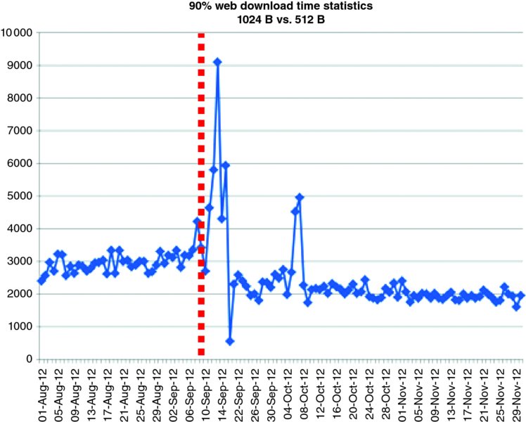
Figure 12.17 Web browsing user experience improvement with shorter buffers
Longer timers result in better user experience due to the extended use of the DCH channel; however, in practice the timers can't be set to values beyond 5 s because they have a significant impact both on battery drain and in network performance – in particular, the uplink noise. A follow up exercise to the one presented, where the inactivity timers were set to 10 s, revealed a significant increase in PS access failures.
When the penetration of Continuous Packet Connectivity (CPC) devices achieves significant levels, it should be possible to further tune these settings to maximize the data user experience with a minimum impact to network resources or battery life.
The exercise in Figure 12.18 shows that the DNS response time would be reduced by over 1 s in case of longer timers; furthermore, thanks to CPC the battery drain would only be 7% higher comparing a baseline 2.6 s timer with an extended 10 s timer. Furthermore, the Uplink Discontinuous Transmission (UL DTX) function of CPC would minimize the amount of uplink interference.
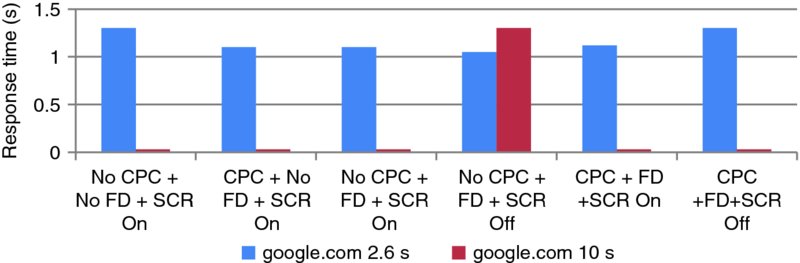
Figure 12.18 DNS response time for two different T2 settings: 2.6 s (light gray) and 10 s (dark gray). CPC = continuous packet connectivity; FD = fast dormancy; SCR = phone screen
12.2.7 Uplink Noise Optimization
Even though data uplink traffic is only a fraction of the volume transmitted in the downlink direction, the current UMTS systems have been unexpectedly suffering from uplink capacity limitations, typically detected in the form of excessive uplink interference or uplink noise.
In most of the cases, operators will try to maintain the network capacity when uplink capacity limits are approached, in the same way that they deal with traditional 2G cellular network congestion by:
- implementing cell splits;
- carrier additions;
- downtilting of antennas;
- traffic redirection between layers and cells;
- and incorporating DAS systems into their networks where applicable.
Although these methods are able to resolve uplink network congestion, they are all costly solutions and do not tackle the root cause of uplink noise rise.
With the introduction of HSUPA, particularly HSUPA with the 2 ms TTI feature, uplink noise rise in many networks was seen to increase. Many operators expected this to occur since the inclusion of HSUPA traffic in a cell allowed for an 8 to 10 dB noise rise (dependent on the network design) above the thermal noise floor to fully obtain the benefits of HSUPA.
Furthermore, the Release 6 HSUPA standards were designed to transfer high bitrate data streams for extended periods of time; however, with the explosion of smartphone traffic in the last few years, it became clear that the existing methods were not optimized for the chatty traffic pattern that is typical of smartphones. This chattiness generates a continuum of small packets flowing to the NodeB from multiple simultaneous locations, which makes it hard to control the interference level in the uplink.
The main impact of high uplink noise is the reduction of the cell coverage, which will be reflected in an increase of packet access failures, as Figure 12.19 illustrates. In this example, when the uplink noise reaches average hourly values beyond 8 dB, the number of access failures increases significantly, both for voice and data connections.
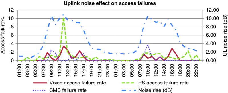
Figure 12.19 Impact of UL noise on access failure rate
The increase in uplink noise will not only affect the performance of that particular cell, but also of adjacent cells, since the mobiles that are attached to it will transmit at a higher power, thus increasing the interference floor of nearby sectors.
Given the importance of uplink noise in smartphone HSPA+ networks, this topic is discussed in various chapters in the book: Chapter 13 provides further details on smartphone chatty profiles, Chapter 11 provided some insight around the relation between the number of connected users and uplink noise, and Chapter 4 discussed some of the HSPA+ features that will help mitigate uplink noise problems in the future, such as the use of CPC and enhanced FACH/RACH. This section provides further analysis on the causes of uplink noise, and some practical methods to mitigate this problem in current networks.
12.2.7.1 Uplink Noise Rise Causes
There are two main reasons for excessive uplink noise in HSPA+ networks:
- a power overhead due to the inefficient design of the uplink channel (DCH), which will cause high levels of interference even in situations where there is no data transmissions; and
- power race scenarios that can be triggered by various causes, including near-far effects and system access with too high power, among others.
Figure 12.20 summarizes an analysis conducted at 3GPP in the context of Continuous Data Connectivity (CPC), which shows the overhead caused by the DPCCH of inactive HSUPA users. In this example, a sector with 30 users in DCH state would deplete the available capacity, even when they are not transmitting any data at all. This analysis is related to the analysis shared in Chapter 11, Section 11.4.3, which shows the relation between UL noise and the number of active users in a sector.
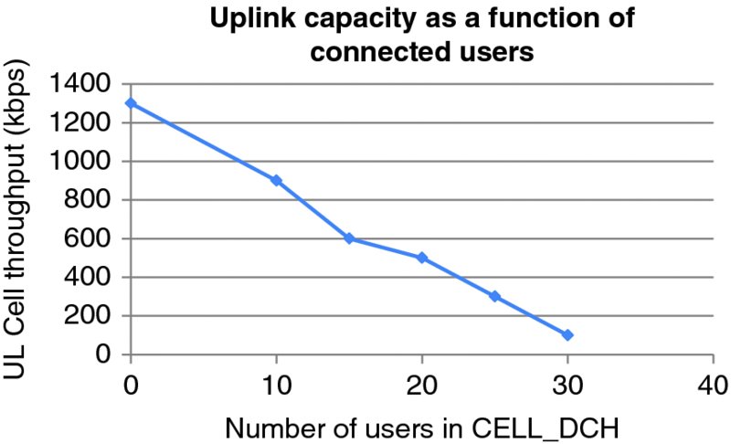
Figure 12.20 Simulation of the reduction of cell capacity with number of connected users (no data). Data from [1]
The most effective method to combat this problem is to adjust the RRC state transition parameters; in particular, reduce the T1 timer as will be discussed later in Section 12.2.7.2.
The introduction of HSUPA users in a sector will also generate a power race between these and the existing voice traffic in the sector: the increase in noise causes the R99 users to no longer meet their uplink EbNo, SIR targets, which results in the failure to meet the BLER targets for the bearers – the system response is to increase the uplink power for each R99 bearer, which causes an increase in the overall uplink system noise. Figure 12.21 shows an example of a congested sector, in which it can be observed how the power of the R99 channels stays typically around 2 dB above the designed uplink load threshold.
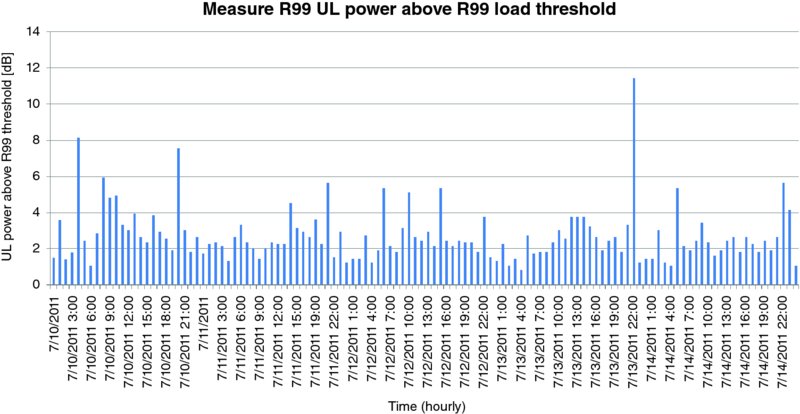
Figure 12.21 Additional uplink power used by R99 channels when HSUPA traffic is present
Following a similar trend, uplink RACH power for UEs will also be higher in a cell with E-DCH bearers, and given the fact that the RACH power does not have an effective power control mechanism, this may cause instantaneous uplink power spikes.
In general, the HSUPA system is highly sensitive to uplink power spikes, which may generate power race conditions such as the one described before. The following describes some of the scenarios that can generate these power spikes.
A wireless system based on spread spectrum will suffer from inter-cell interference in both the uplink and the downlink. When a UE approaches a cell boundary, the power received by the non-serving cell will be within a few dBs of the serving cell. This problem is more pronounced with the introduction of HSUPA, where soft handover is not widely utilized. One approach to dealing with this issue is to downgrade the uplink scheduling TTI based on an Ec/No threshold from 2 to 10 ms, allowing for less power to be used in the UL. Another option is to control the soft handover parameters for HSUPA service, expanding the triggering of cell addition as well as the time to trigger additional windows, in order to control the interferer. This will, however, have an impact on the NodeB baseband resources.
A similar problem is caused by building shadowing, where a UE is connected to one cell but due to mobility and shadowing (such as moving around a building) finds itself within the footprint of a new cell. This results in a significant amount of power being received in the new cell before the UE can enter into soft handover and the interference brought under control.
Figure 12.22 shows the results of this effect – a cell carrying no UE traffic and experiencing high uplink noise in the beginning part of the trace before the UE changes cells. A plot of the UE TX power during the cell change is shown in Figure 12.23.
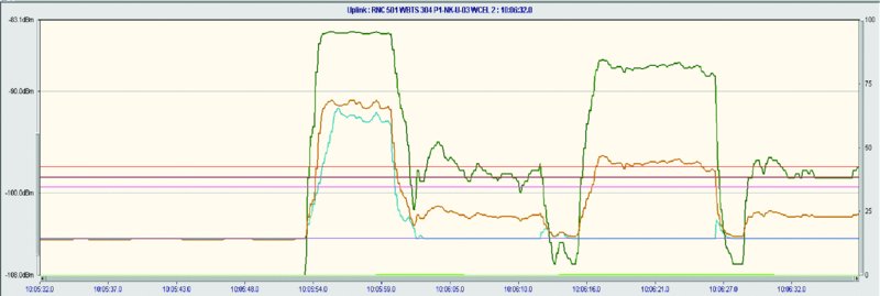
Figure 12.22 Power measurement from live sector showing near–far problem

Figure 12.23 Illustration of UE Tx power peak during HS cell change
In this example, prior to cell change the UE TX power ramps up to 14 dBm before reducing to −15 dBm post cell change.
In many cases, it is not possible to avoid those uplink spikes; however it is possible to control how the system deals with these spikes. Section 12.2.7.3 presents an example in which the system parameters are adjusted to limit the reaction of the devices in the cell, thus effectively mitigating the consequential increase in uplink noise.
12.2.7.2 Adjustment of State Transition Timers
As previously indicated, an effective way to reduce uplink noise in congested cells is the optimization of the RRC state transitions parameters, in particular the reduction of the T1 timer, which controls the transition from Cell_DCH to Cell_FACH state. A reduction in T1 timers will lead to fewer erlangs which, as discussed in Chapter 11, Section 11.4.3, is helpful in reducing the noise rise, but will also increase the signaling load in the network. Furthermore, as indicated in Section 12.2.6, a reduction in these timers will result in a longer connection delay, which will impact the user experience. Unfortunately, in most vendor implementations these settings are configured at the RNC level and it is therefore not possible to reduce the timers only in sectors with extreme congestion.
Figure 12.24 illustrates the impact of modifying the T1 timer from 8 s down to 3 s in a live RNC. The chart represents the uplink Received Total Wideband Power (RTWP) distribution for the top 5 loaded cells in the RNC, before and after the change.
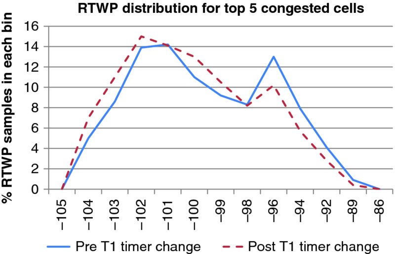
Figure 12.24 Impact of inactivity timer optimization on UL noise
As the figure indicates, there is a significant reduction of uplink noise after the change, as can be seen in the reduction of samples between −98 and −83 dBm. As a consequence of the optimization, the following aspects were improved in the network:
- HSUPA packet session access failure rate was reduced from 10.8 to 3.8%.
- The usage of the UL R99 channel was reduced (80% reduction in triggers due to reaching the limit of HSUPA users).
- Reduction in NRT SHO overhead from 25.7 to 23.8%.
- 13 to 45 mA reduction in battery utilization, depending on device type and user activity.
The drawbacks of this change include:
- Higher (2–3%) RNC processing load due to increased signaling.
- An increase in utilization of FACH/RACH channels.
- Increase in connection latency.
12.2.7.3 Adjustment of Filter Coefficients
In some infrastructure vendors, one effective method to reduce the uplink noise rise caused by these effects is to modify the filter coefficient length used by the NodeB to aggregate the uplink noise rise measurement. By extending the filter coefficient, significant improvements in the uplink noise rise can be obtained. As shown in Figure 12.25, the uplink noise spiking caused by the shorter filter coefficient is eliminated and a smoother, less “spiky” noise measurement is obtained.

Figure 12.25 Filter coefficient adjustment and impact on the measured noise floor
The modification of the filter coefficient has a direct impact on the PRACH outer loop power control, and can introduce more stability into the system. If we refer to the initial PRACH power calculation:
The filter coefficient controls the way the UL interference component of this formula is calculated by the NodeB and transmitted to the mobiles via the SIB7 information block. A conservative setting of the filter coefficient makes the system less susceptible to instantaneous modifications in uplink noise.
Statistical analysis of a real network has shown the following improvements in the RTWP with the introduction of changing this value, as shown in Figure 12.26.
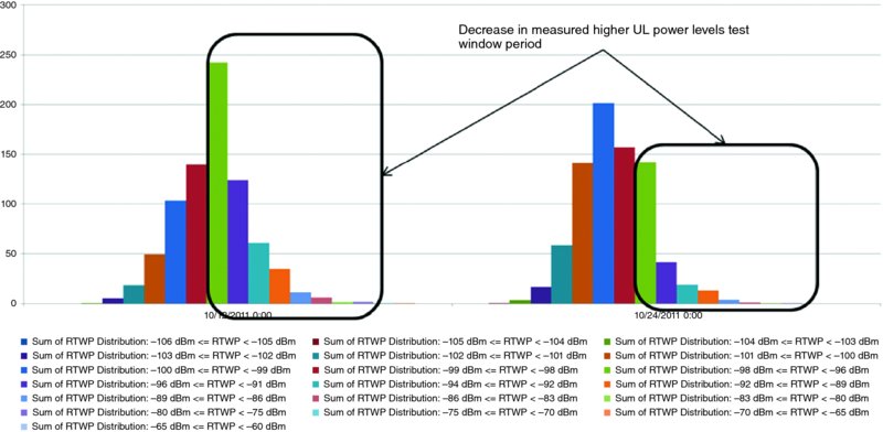
Figure 12.26 RTWP distribution in the test cluster. Left: with default (shorter) coefficients; right: after parameter change
12.2.7.4 Adjustment of PRACH Parameters
Care should also be taken to tune the initial PRACH target settings. Lab testing has shown that, when these values are not optimally adjusted, excessive spiking occurs when there are small coupling losses between the UE and the network as shown below in Figure 12.27
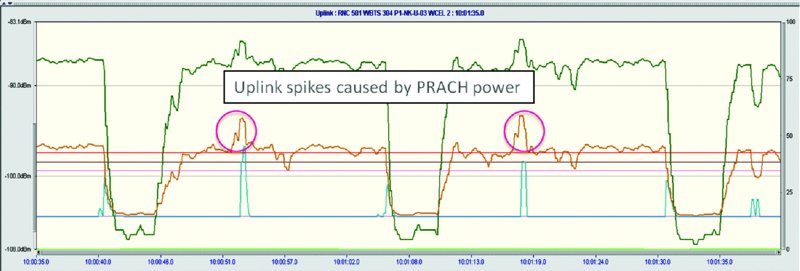
Figure 12.27 Spiking in uplink noise due to initial PRACH access attempts; circles show noise spiking effects
Many network operators approach PRACH power settings with the goal of ensuring reduced call setup times. Their approach is therefore to maximize the power used in the initial PRACH settings which ensures an access grant on the first attempt. In a spread spectrum network this approach has a negative impact on the uplink shared resource.
In a study conducted on a live network cell, adjusting the initial PRACH parameters showed immediate relief from excessive uplink noise rise (Figure 12.28).
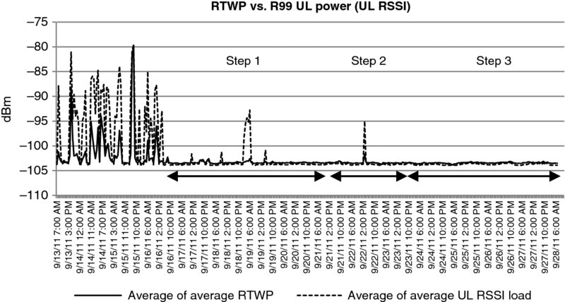
Figure 12.28 Impact of PRACH parameter optimization on UL noise
Table 12.5 defines the parameter sets that were used in the above study. PRACH optimization needs to be done cautiously as it has an impact on cell coverage and very aggressive values could result in missed calls. When analyzing different impacts, special care should be taken to ensure that traffic is not being lost due to the smaller sector footprint. This can be checked through drive tests or with the help of geolocation tools.
Table 12.5 Summary of PRACH parameter changes
| Parameter | Baseline | Step 1 | Step 2 | Step 3 |
| Required PRACH C/I | −25 dB | −28 dB | −30 dB | −33 dB |
| PRACH preamble step size | 2 dB | 1 dB | 1 dB | 1 dB |
| RACH preamble retransmissions | 32 | 16 | 16 | 16 |
| RACH preamble cycles | 8 | 1 | 1 | 1 |
| Power offset after last PRACH preamble | 0 dB | 2 dB | 2 dB | 2 dB |
In this study, the biggest improvement occurred after step 1, the contributor to this change is the required PRACH carrier to interference target. The other steps deal with further decreasing the required carrier to interference ratio; however, not much further improvement is obtained for this change.
Combining the filter coefficient together with the PRACH settings, a significant amount of the noise that exists in the uplink can be controlled.
12.3 Optimization Tools
With the increase of technology complexity the planning and maintenance of the network has become increasingly difficult; however, new and powerful engineering tools have been designed to help the engineers in their daily tasks. In this section we discuss three of the most interesting tools that are available today, which can help operators improve their network operational efficiency and performance: geolocation, user tracing tools, and self-organizing network (SON) tools.
12.3.1 Geolocation
Geolocation tools can help provide traffic positioning data to be used for network planning and dimensioning. As discussed in Chapter 11, network performance and capacity are always maximized when the cell sites can be located near the traffic sources. Additionally, the geolocation tool can be used to:
- Evaluate impact from a network change, by analyzing geolocated metrics such as RSCP and Ec/No.
- Help pinpoint problem areas in a network, typically masked by macroscopic network KPIs.
- Provide geolocated data to feed other tools, such as planning, Automatic Cell Planning (ACP) and SON tools.
There are two types of tool that can provide geolocation information: the first type requires a special client embedded in the handset device that reports statistics collected at the application layer with GPS accuracy; one example of this tool is carrier IQ. This first type of tool provides very good geolocation accuracy, but limited radio information.
The second type of tool can provide detailed RF metrics, such as pilot power, Ec/No, and RRC events such as handovers. This information is gathered from special RNC trace interfaces that stream UE measurements and events, such as Ericsson's General Performance Event Handling (GPEH) or NSNs MegaMon. Since the mobiles don't report their location, these tools estimate it based on triangulation information and timing advance. The accuracy improves with a larger number of neighbors; therefore there is typically higher accuracy in dense urban environments (around 100 m), as compared to suburban (around 300 m) and rural environments (up to 1000 m).
Figure 12.29 shows an example network in which a signal strength map has been built based on geolocation data. Traffic information has also been overlayed on the map to show the areas with higher network traffic.
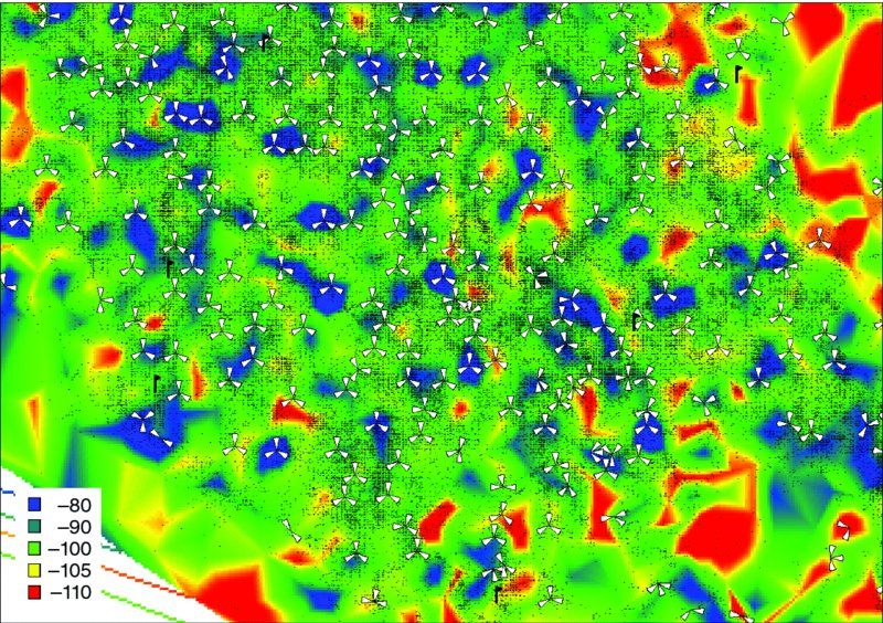
Figure 12.29 Example of a geolocation exercise. The shades of gray represent the pilot signal strength, and the black dots the location of the traffic samples
12.3.2 User Tracing (Minimization of Drive Tests)
The user tracing tools permit one to visualize RF metrics and Layer 3 messages from any mobile in the network, providing a subset of the functionality than that of a drive test tool, with the convenience of remote operation.
A similar use case has been standardized for LTE systems, and is referred to as “Minimization of Drive Tests” or MDT. In the case of UMTS, the functionality is non-standard, but most infrastructure vendors provide a wealth of trace information through proprietary interfaces – the same one that was mentioned in the case of the geolocation tool. Consequently, often both tools – geolocation and user tracing functionality – are offered within the same framework.
The main uses of the MDT tools are:
- Substitution for drive testing, which can result in significant savings in engineering resources.
- Generation of real-time alerts based on network or user KPIs (dropped calls, access failures, etc.).
- Troubleshooting support to customer care. These tools can typically save historical trace data, which can be used in case a specific customer issue needs to be analyzed.
- Support for marketing uses, based on customer behavior.
Figure 12.30, taken from one of the leading tools in this space, shows the typical capabilities of this type of tool. As can be observed, the engineer can monitor specific geographical areas, identify issues, and drill down into the trace of the specific subscriber that has suffered the problem. Historical data from the subscriber is also available to understand what happened to the connection before the specific problem occurred.
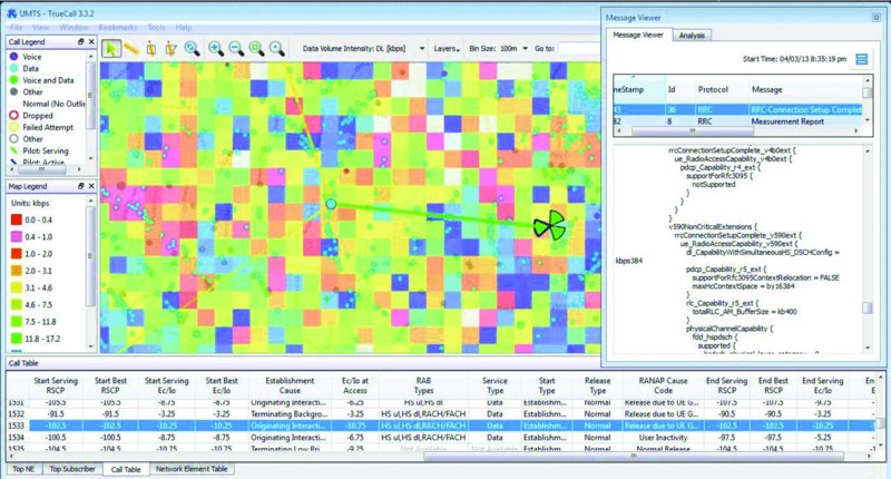
Figure 12.30 Snapshot of remote tracing tool, showing user events and traces. Reproduced with permission of Newfield Wireless
As indicated earlier, these tools nowadays need to operate on closed, proprietary interfaces that have been defined by the infrastructure vendors. This complicates the integration and maintenance of such tools, and makes them dependent on the willingness of the infrastructure vendors to share their format information.
12.3.3 Self Organizing Network (SON) Tools
While network technologies have been evolving very rapidly, the operational tools that the field engineers utilize in their daily activities are still very labor intensive. A significant amount of the engineer's work day is spent in manual tasks, reports, and troubleshooting activities, which prevents them from concentrating on proper optimization activities, which are often very time-consuming.
As discussed in many instances in this chapter, in order to achieve optimum efficiency and performance, the network should be configured on a cell by cell basis. In some cases, it should be configured differently at specific times of the day, since traffic distributions can change dramatically in certain conditions. However, it is practically impossible to manually design and manage so many changes, and it risks human error due to the complexity of the task.
This challenge was widely discussed during the introduction of the LTE technology, and considerable effort has been put into a new concept called “Self Organizing Networks,” whose ultimate goal is to improve the operational efficiency of the carriers through increased network automation. Some of the benefits of utilizing SON techniques are:
- Permits operators to optimize many aspects of the network at once, with minimal or no supervision.
- Provides fast and mathematically optimum configurations of the network.
- Continuous network optimization, adapting to changes in the environment.
- Optimization of each sector independently, ensuring an optimum configuration in each and every location and improving overall network efficiency.
- Permits assigning different configuration strategies at different times of the day.
The concept of self organizing networks can be applied to any network technology, and in the case of HSPA+ some SON algorithms are readily available from infrastructure vendors, to support mainly integration tasks such as NodeB plug and play, or automatic neighbor configuration. Additionally, there are third-party companies that offer automatic optimization solutions that can connect to the operator's data sources to extract the relevant KPIs and output an optimized set of parameters for that network. These solutions are becoming increasingly popular as they deliver on the promised performance and operational efficiencies.
Below is a recommended list of features that the SON tool should provide:
- Support for fully automated, closed-loop mode as well as open-loop mode for test purposes.
- Support for automatic import/export of data. The SON tool should be able to handle Configuration Management (CM) and Performance Management (PM) data from the OSSs, as well as streaming trace data such as GPEH and Megamon feeds.
- Support for advanced data management functions, including functions to analyze data trends, and the ability to provide parameter rollback mechanisms.
- Fast processing and reaction time to near-real time data.
- Coordination mechanisms for different algorithms and parameters.
- Configurable optimization strategies.
12.3.3.1 SON Algorithms for HSPA+
The optimization algorithms will typically try to find a balance between coverage, capacity, and quality, depending on a certain policy that can usually be configured by the operator. To achieve this, the SON tool typically modifies network parameters that are configurable through the OSS, while for example, the Automatic Cell Planning (ACP) tool deals primarily with RF parameters such as antenna tilts, azimuth, height, and so on. However, as SON tools have become more sophisticated, the boundary between these tools has become blurred, and now it is possible to find SON algorithms that optimize certain RF parameters, such as pilot powers and antenna tilts. Table 12.6 summarizes some of the HSPA+ SON strategies that can be found in today's tools.
Table 12.6 Table with automated 3G strategies
| Automated planning, configuration, and integration | |
| NodeB integration support | 3G automatic neighbors |
| Automatic NodeB rehomes | Parameter consistency enforcement |
| Automated optimization | |
| Cell outage detection and compensation | Energy savings |
| 3G mobility optimization | Automatic load balancing |
| Automatic CCCH optimization | Coverage and interference optimization |
| Automated performance monitoring and troubleshooting | |
| Automatic performance reports | Real-time alerts |
| Detection of crossed antenna feeders | Cell outage detection and compensation |
| Automatic sleeping cell detection and resolution | |
The following section provides a high-level description of the most interesting algorithms for automatic 3G optimization.
UMTS Automatic Neighbors (ANR)
This algorithm configures neighbors of a 3G cell to try and minimize dropped calls due to missing neighbors and UL sync issues. Most existing modules will configure intra-frequency, inter-frequency, and inter-RAT neighbors to GSM, and will keep the neighbor list within the limits imposed by the technology or vendor implementation. In certain implementations, this module can operate in near real time taking input from RAN traces, which can be very helpful during cell outages.
Automatic Load Balancing
These algorithms will try and adjust the sector footprint, handover weights, and inter-layer configuration parameters to distribute the load in case of high congestion in one specific hotspot area. The goal is to maximize service availability (limit access failures) and increase throughput fairness for all customers, irrespective of their geographical location. There are two flavors of load balancing mechanisms, one that reacts quickly to sudden changes in traffic, and one that tries to adjust the network configuration based on long-term traffic characteristics.
Automatic Sleeping Cell Resolution
Sleeping cells are sectors which stop processing traffic for no apparent reason, and for which no alarm is generated. The sleeping cell detection algorithm identifies a sleeping cell based on certain performance criteria and resets the cell accordingly.
Coverage and Interference Optimization
This module adjusts the footprint of the cells by modifying antenna tilts (in case of RET capable) and powers to (i) eliminate coverage holes in the area, (ii) minimize inter-sector interference, and (iii) minimize the amount of power used in the cluster. In some cases, the algorithm will use geolocation information to improve the accuracy of the decision. If antenna ports are being shared by more than one technology, then decisions for tilts need to be assessed for all network layers that share that path.
12.3.3.2 Results from SON Trials
HSPA+ SON tools are commercially deployed in a number of networks today. The examples in this section are extracted from test results of these tools in a live network.
The following example illustrates the use of a SON tool during a network recovery situation. The network presented was impacted by a heavy storm which caused a very large number of cell outages in the area; when this happened, the number of drops due to bad neighbor configuration skyrocketed and the engineers were spending a large amount of their time configuring neighbor relations, which took away time from other network recovery efforts. Three days after the event, a SON tool was activated in the area, which took care of automatic neighbor configuration in the network. Figure 12.31 shows the relevant network statistics and time savings.
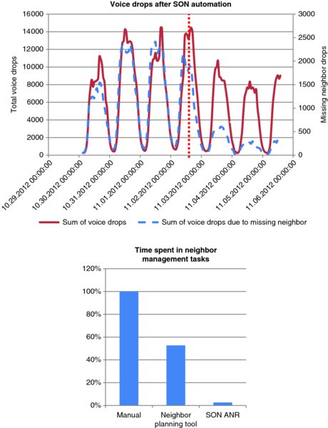
Figure 12.31 Results from SON ANR execution during massive cell outages situation
As can be seen, the number of voice drops was dramatically reduced immediately after the activation of the ANR solution. Due to the dramatic cell outage situation, the amount of drops due to missing neighbors accounted for almost 20% of the total number of drops; after the tool was activated, this percentage was reduced to less than 4%. And most importantly, as indicated on the chart on the right, all this improvement was obtained with no intervention from the engineering crew, except for the initial configuration required.
In the next example, a SON tool was activated in two live RNCs in a market for a month. Several SON algorithms were run continuously, including:
- automatic parameter enforcement;
- plug and play (configuration of new sectors);
- ANR;
- coverage and interference optimization.
During the trial period, other RNCs in the market were used to track any possible changes in the network, such as natural traffic growth, seasonality effects, and so on.
Figure 12.32 shows the reduction in drops in one of the RNCs (RNC4) once the SON tool was activated. It should be noted that the tool runs autonomously, gathering KPIs every 15 min interval, and is capable of implementing parameter modifications at that rate if necessary. The Drop Call Rate (DCR) chart shows a spike corresponding to an outage in the network that happened before the tool was activated.

Figure 12.32 Reduction in voice drop call rate in one of the trial RNCs
The second RNC (RNC2) was activated one week later with similar performance improvements. Given the fact that parameter changes are implemented gradually, which results in a slow slope in performance improvement, this second RNC showed lower gains at the time of the analysis.
Table 12.7 summarizes the performance results, comparing weekly statistics before and after the tool was activated in each of the RNCs.
Table 12.7 Improvement in main KPIs after SON activation
| KPIs | RNC4 (%) | RNC2 (%) | Other RNCs (%) |
| Voice drop call rate gain | 21 | 14 | 0 |
| Voice access failure rate gain | 30 | 10 | −14 |
| Voice traffic gain | 8.2 | 9.2 | 7 |
| Voice IRAT gain | 11 | 15 | 2.2 |
| Data drop call rate gain | 14.5 | 19 | −1.3 |
| Data access failure rate gain | 56.3 | 2.4 | 11.7 |
| Data traffic gain | 5.6 | 7.3 | 5.1 |
| Data IRAT gain | 2.1 | −2.9 | 2.4 |
| Data throughput gain | 6.3 | 9.9 | 3.5 |
As the results show, the SON tool was able to improve in all main KPIs, while still capturing more traffic than the rest of RNCs in the market. Even more interesting is the fact that calls to customer care in the trial area were reduced by about 15%.
12.3.3.3 Evolution of the SON Architecture
In the long run, SON tools will become a central piece in the network operations process, and will likely evolve into a more complex architecture in which it interacts with other engineering tools, in addition to the OSS. The leverage of big data technologies will help facilitate this paradigm shift. The following aspects are facilitated by an evolved SON architecture:
- Increased scope of data sources and network elements, expanding from OSS to operator specific units, such as work order and inventory databases.
- Simplified data extraction and consolidation that is used by the multiple tools to pull data and configuration information, and push new configurations as required by the automated tasks. It should provide advanced filtering capabilities as well as data storage, and the ability to work with historical data as well as near real-time.
- The SON tool will interact with existing engineering tools that add value to the system, but don't operate in an automatic fashion. For instance, the tool may receive special alerts that are generated in real time by the MDT tool, and react accordingly.
- New, custom automation tasks can be defined and created in the form of SON plugin modules, that can be scheduled to run in background, either periodically or reacting to upcoming events from the SON framework or other tools.
Figure 12.33 illustrates this concept.
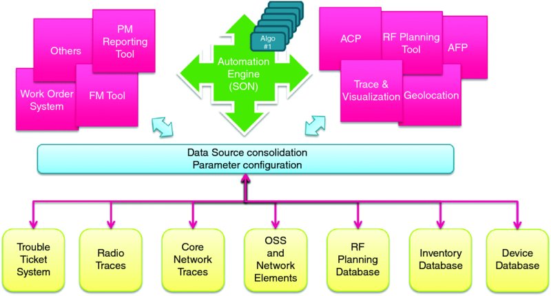
Figure 12.33 Advanced SON management architecture
The above mentioned architecture would facilitate an increased level of network automation. It will enable a transition from network-centric SON actions, which are typically based on aggregated node KPIs, to customer-centric specific actions, including app-level optimization.
Figure 12.34 illustrates an example interaction that would be possible with this architecture. In this example, the SON system detects congestion in certain areas, and notifies an application server that is generating excessive traffic in the area – the app server will modify the service quality for the users in the affected areas, which will in turn alleviate the congestion in the network.
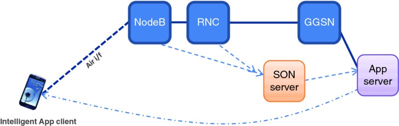
Figure 12.34 Example of advanced SON interactions
12.4 Summary
This chapter has presented the main focus areas for optimization in commercial HSPA+ networks, including neighbor management, antenna and power configurations, handovers, and radio state transitions.
A special section has been devoted to analyzing the uplink noise rise problem, which is probably the most challenging optimization task in networks with a large number of smartphones, and several techniques have been discussed to help mitigate the problem.
Finally, several useful engineering tools have been discussed, including self organizing network and MDT tools, which would greatly help during the optimization and troubleshooting of the HSPA+ networks.
Reference
- 3GPP TR 25.903, “Continuous connectivity for packet data users”, Release 8.