

11
Networks
Elizabeth L. Ogburn and Alexander Volfovsky
CONTENTS
11.1 Introduction .................................................................... 171
11.2 Network Models ................................................................ 173
11.2.1 Erdos–Renyi–Gilbert Model ........................................... 173
11.2.2 Stochastic Blockmodel ................................................. 174
11.2.3 General Latent Space Model .......................................... 176
11.2.4 Testing for Network Structure ......................................... 177
11.2.4.1 Bickel and Sarkar (2013) Main Result ..................... 177
11.2.4.2 Volfovsky and Hoff (2014) Main Result .................... 177
11.3 Observations Sampled from Network Nodes ................................... 178
11.3.1 Terminology and Notation ............................................ 179
11.3.2 Experiments in Networks .............................................. 179
11.3.2.1 Fisherian Hypothesis Testing .............................. 180
11.3.2.2 Estimation of Causal Effects in Randomized Experiments
on Networks ................................................ 181
11.3.3 Observational Studies ................................................. 182
11.3.3.1 Peer Effects ................................................. 182
11.3.3.2 Instrumental Variable Methods ............................ 183
11.3.3.3 Dependence ................................................. 184
11.3.3.4 Targeted Maximum Loss-Based Estimation for Causal
Effects in Networks ......................................... 185
11.4 Discussion and Future Directions .............................................. 185
References ............................................................................. 186
11.1 Introduction
Networks are collections of objects (nodes or vertices) and pairwise relations (ties or edges)
between them. Formally, a graph G is a mathematical object composed of two sets: the
vertex set V = {1,...,n} lists the nodes in the graph and the edge set E = {(i, j):i ∼ j}
lists all of the pairwise connections among the nodes. Here ∼ defines the relationship between
nodes. The set E can encode binary or weighted relationships and directed or undirected
relationships. A common and more concise representation of a network is given by the n ×n
adjacency matrix A,whereentrya
ij
represents the directed relationship from object i to
object j. Most often in statistics, networks are assumed to be unweighted and undirected,
resulting in adjacency matrices that are symmetric and binary: a
ij
= a
ji
is an indicator of
whether i and j share an edge. A pair of nodes is known as a dyad; a network with n nodes
171
172 Handbook of Big Data
has
n
2
distinct dyads, and in an undirected graph, this is also the total number of possible
edges. The degree of a node is its number neighbors, or nodes with which it shares an edge.
In a directed network, each node has an in-degree and an out-degree; in an undirected
network, these are by definition the same. Some types of networks, such as family trees
and street maps, have been used for centuries to efficiently represent relationships among
objects (i.e., people and locations, respectively), but the genesis of the mathematical study
of networks and their topology (graph theory) is usually attributed to Euler’s 1741 Seven
Bridges of K¨onigsberg (Euler, 1741).
Beginning with Euler’s seminal paper and continuing through the middle of the twentieth
century, the formal study of networks or graphs was the exclusive domain of deterministic
sciences such as mathematics, chemistry, and physics; its primary objectives were the
description of properties of a given, fixed graph, for example, the number of edges, paths,
or loops of a graph or taxonomies of various kinds of subgraphs. Random graph theory was
first introduced by the mathematicians Erdos and Renyi (1959). A random graph is simply
a random variable whose sample space is a collection of graphs. It can be characterized
by a probability distribution over the sample space of graphs or by the graph-generating
mechanism that produces said probability distribution. Random graph theory has become a
vibrant area of research in statistics: random graph models have been used to describe and
analyze gene networks, brain networks, social networks, economic interactions, the formation
of international treaties and alliances, and many other phenomena across myriad disciplines.
Common to all of these disparate applications is a focus on quantifying similarities and
differences among local and global topological features of different networks. A random
graph model indexes a probability distribution over graphs with parameters, often having
topological interpretations; the parameters can be estimated using an observed network
as data. Parameter estimates and model fit statistics are then used to characterize the
topological features of the graph. We describe some such models and estimating procedures
in Section 11.2.
Over the past 5–10 years, interest has grown in a complementary but quite different
area of network research, namely the study of causal effects in social networks. Here,
the network itself is not causal, but edges in the network represent the opportunity for
one person to influence another. Learning about the causal effects that people may have
on their social contacts concerns outcomes and covariates sampled from network nodes—
outcomes superimposed over an underlying network topology—rather than features of the
network topology. A small but growing body of literature attempts to learn about peer
effects (also called induction or contagion ) using network data (e.g., Christakis and Fowler,
2007, 2008, 2010): these are the causal effects that one individual’s outcome can have
on the outcomes of his or her social contacts. A canonical example is infectious disease
outcomes, where one individual’s disease status effects his or her contacts’ disease statuses.
Interference or spillover effects are related but distinct causal effects that are also of interest
in network settings; these are the causal effects that one individual’s treatment or exposure
can have on his or her contacts’ outcomes. For example, vaccinating an individual against
an infectious disease is likely to have a protective effect on his or her contacts’ disease
statuses.
Simple randomized experiments that facilitate causal inference in many settings cannot
be applied to the study of contagion or interference in social networks. This is because the
individual subjects (nodes) who would be independently randomized in classical settings
do not furnish independent outcomes in the network setting. In Section 11.3, we describe
recent methodological advances toward causal inference using network data. Before that,
in Section 11.2, we describe some current work on probabilistic network generating models.
While it is possible to be relatively complete in our survey of the literature on causal
inference for outcomes sampled from social network nodes, the literature on network
Networks 173
generating models is vast, and we limit our focus to models that we believe to be appropriate
for modeling social networks and that we see as potential tools for furthering the project of
causal inference using social network data.
Networks are inarguably examples of big data, but just how big they are is an open
question. Big data often points to large sample sizes and/or high dimensionality. Networks
can manifest both kinds of bigness, with a tradeoff between them. On the one hand, a
network can be seen as a single observation of a complex, high-dimensional object, in which
case sample size is small but dimensionality is high. On the other hand, a network can be
seen as comprising a sample of size on the order of the number of nodes or the number
of edges. In this case, sample size is large but complexity and dimensionality are less than
they would be if the entire network were considered to be a single observation. In reality,
the effective sample size for any given network is likely to lie somewhere between 1 and the
number of nodes or edges. We are aware of only one published paper that directly tackles the
question of sample size for network models: Kolaczyk and Krivitsky (2011) relate sample
size to asymptotic rates of convergence of maximum likelihood estimates under certain
model assumptions. A notion of sample size undergirds any statistical inference procedure,
and most of the models we describe below inherently treat the individual edges or nodes as
units of observation rather than the entire network. In some cases, this approach ignores
key structure and complexity in the network and results in inferences that are likely to be
invalid. We do not explicitly focus on issues of sample size and complexity in this chapter,
but note that the tradeoff between network-as-single-complex-object and network-as-large-
sample is a crucial and understudied component of statistics for network data.
11.2 Network Models
Different network models are designed to capture different levels of structure and variability
in a network. We discuss three models in increasing order of complexity: the Erdos–Renyi–
Gilbert model, the stochastic blockmodel and the latent space model. For each of these three
models, we describe the parameters and properties of the model and, where appropriate,
propose estimation and testing procedures to fit the model to observed network data. For
more extensive surveys of the literature on random graph models, see Goldenberg et al.
(2010) and Kolaczyk (2009).
11.2.1 Erdos–Renyi–Gilbert Model
The first random graph model, developed simultaneously by Paul Erdos and Alfred Renyi
and by Edgar Gilbert, considers a random graph G with a fixed number of nodes n = |V |
and a fixed number of undirected edges e = |E| that are selected at random from the pool
of
n
2
possible edges. This induces a uniform distribution over the space of graphs with n
nodes and e edges (Erdos and Renyi, 1959; Gilbert, 1959). A slight variation on this model
fixes n but only specifies e as the expected number of edges in an independent sample—that
is, the probability of any particular edge is given by p = e/
n
2
,sothate is the expected
but not necessarily exact number of realized edges. Under both of these formulations, the
primary objects of interest are functions of p and n; therefore, these models collapse all
of the possible complexity in a network into two parameters and provide only a high-level
overview of the network.
Much of the early work on the Erdos–Renyi–Gilbert model concentrated on its
asymptotic behavior. One of the most celebrated results describes a phase change in the
structure of Erdos–Renyi–Gilbert random graphs as a function of expected degree λ = pn,
174 Handbook of Big Data
namely the almost sure emergence of a giant component as n →∞when λ converges to a
constant greater than 1. A giant component is a connected component (a subgraph in which
all nodes are connected to one another by paths) that contains a strictly positive fraction of
the nodes. According to the phase change results, all other components are small in the sense
that none of them contain more than O(log n)nodes.Ifλ converges to a constant smaller
than 1, then almost surely all components are small in this sense. Finally, for λ =1,the
largest component is almost surely O(n
2/3
) (Durrett, 2007). While this is a simplistic model
for real-world networks, the emergence of the giant component is of practical importance
when performing inference.
Perhaps the most significant criticism of this model is that real-world networks generally
do not exhibit constant expected degrees across nodes; power law degree distributions
(Barab´asi and Albert, 1999; Albert and Barab´asi, 2002), and departures from those (Clauset
et al., 2009) are thought to be especially common. A natural extension of the Erdos–
Renyi–Gilbert model, allowing for a power-law and other degree distributions, partitions
the nodes into groups having different expected degrees, essentially interpolating several
different Erdos–Renyi–Gilbert graphs (Watts and Strogatz, 1998). However, these models
can become unwieldy; for example, efficiently generating a simple graph with a user-specified
degree distribution requires sequential importance sampling (Blitzstein and Diaconis, 2011).
Additionally, as we will see in Section 11.2.3, nonconstant degree distributions can be
accommodated very intuitively by the latent space model.
A sample from an undirected Erdos–Renyi–Gilbert model with n =20nodesandedge
probability p = .25 is displayed in the first panel of Figure 11.1. The expected degree
for each node in the graph is np = 4; the observed average degree is 5.5. Estimation of the
probability of edge formation under this model is straightforward via the binomial likelihood
p
e
(1 − p)
(
n
2
)
−e
,wheree is the observed number of edges, and in this case ˆp = .289. The
simplicity of this model and estimation procedure make it extremely appealing for inference
when we cannot observe the full network, as the marginal distribution of any subgraph is
easily computed, but the lack of any structure on the nodes and their degrees ensures that
this model a simplification of reality in most cases.
11.2.2 Stochastic Blockmodel
A higher level of model complexity is achieved by the stochastic blockmodel (Holland et al.,
1983; Nowicki and Snijders, 2001; Wang and Wong, 1987), which recognizes that a given
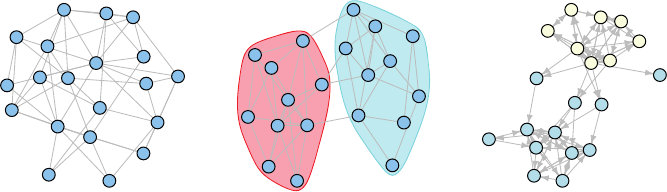
(a) (b) (c)
FIGURE 11.1
Networks generated using the three models described in Section 11.2. They are: (a) an
Erdos–Renyi–Gilbert graph with p =1/2; (b) a stochastic blockmodel with probability
matrix P =
0.50.2
0.20.4
; and (c) a directed latent space model based on the latent variable
s
ij
= α
i
+ α
i
α
j
+
ij
where α
i
,
ij
iid
∼ normal(0, 1).
Networks 175
network node is more likely to be connected to some nodes than to others (e.g., because it
is more similar to some nodes than to others). This is codified in the assumption that the
n nodes in a network are separated into k<nnonoverlapping groups and the relationship
between any two nodes depends only on their group memberships. Nodes that belong
to the same group are stochastically equivalent—that is, probability distributions over
their edges are identical. The Erdos–Renyi–Gilbert model is a special case of a stochastic
blockmodel with k = 1. By introducing structure in the form of multiple groups of nodes, the
stochastic blockmodel captures an additional level of complexity and relaxes the assumption
of identical expected degree across all nodes. While this model is not generally compatible
with power law degree distributions, it is very flexible.
The parameter of a stochastic blockmodel is a k × k probability matrix P ,whereentry
p
ij
is the probability that a node in group i is connected by an edge to a node in group
j. Edges can be directed or undirected. The main constraint on P is that every entry is
between 0 and 1. While p
ij
= 0 or = 1 may be plausible, many estimation procedures
make the assumption that p
ij
is bounded away from 0 and 1. For undirected networks, an
additional assumption is that the matrix P is symmetric (or simply upper triangular), while
for directed networks, this requirement can be relaxed. In the middle panel of Figure 11.1,
we see an undirected network simulated from a two block stochastic blockmodel where the
probability of edges within each block is greater than that between the blocks. Additionally,
one of the blocks has a higher probability of within group edges than the other.
The color coding in the figure clearly demarcates the two groups in the stochastic
blockmodel and it is easy to see that each of the groups can be viewed marginally as
an Erdos–Renyi–Gilbert graph. Given the group labels, we can perform inference as in the
Erdos–Renyi–Gilbert case, treating each class of edges (within each group and between each
pair of groups) individually to estimate the entries of P . However, we rarely know group
membership apriori, making estimation of the stochastic blockmodel parameters much
more complicated, since the group labels must be inferred. There are two main approaches
to this estimation process. The first is a model-driven approach in which group membership
is a well-defined parameter to be estimated jointly with the elements of P ; this approach
can be viewed as a special case of the latent space model (see Section 11.2.3), where the
multiplicative latent effects are k dimensional vectors with a single nonzero entry. The
second approach is a heuristic approach involving spectral clustering. Given the number of
clusters or blocks, k, and an adjacency matrix A, the first step is to find the k eigenvectors
corresponding to the k largest eigenvalues (in absolute value; Rohe et al., 2011) of the graph
Laplacian L (= D
1/2
AD
1/2
,whereD
ii
=
j
a
ij
). Treating the rows of the concatenated
n×k matrix of eigenvectors as samples in R
k
, the next step is to run a k-means algorithm to
cluster the rows into k nonoverlapping sets. These sets estimate the groups of the underlying
stochastic blockmodel, and Rohe et al. (2011) provide bounds on the number of nodes that
will be assigned to the wrong cluster under conditions on the expected average degree as
well as the number of clusters. The power of their result lies in the fact that they allow the
number of clusters to grow with sample size. Choi et al. (2012) developed similar results for
a model-based approach to clustering in stochastic blockmodels. After clustering, estimation
of P is straightforward.
It has recently been shown that stochastic blockmodels can provide a good approxima-
tion to a general class of exchangeable graph models characterized by a graphon: a function
mapping the unit square to the unit interval and representing the limiting probability
of edges in a graph (Airoldi et al., 2013). This suggests that, given the relatively weak
assumption of an exchangeable graph model, a stochastic blockmodel approximation may
lead to approximately valid inference. In other words, despite the simplicity of the stochastic
blockmodel and the fact that the only structure it models is at the group level, it captures
enough structure to closely approximate a large class of exchangeable random graph
models.
..................Content has been hidden....................
You can't read the all page of ebook, please click here login for view all page.