

20
Tutorial for Causal Inference
Laura Balzer, Maya Petersen, and Mark van der Laan
CONTENTS
20.1 Why Bother with Causal Inference? ........................................... 361
20.2 The Scientific Question ........................................................ 363
20.3 The Causal Model .............................................................. 363
20.4 The Target Causal Quantity ................................................... 366
20.5 The Observed Data and Their Link to the Causal Model ..................... 368
20.6 Assessment of Identifiability ................................................... 369
20.7 Estimation and Inference ...................................................... 373
20.8 Interpretation of the Results ................................................... 376
20.9 Conclusion ...................................................................... 377
Appendix: Extensions to Multiple Time Point Interventions ......................... 378
Acknowledgments ...................................................................... 381
References ............................................................................. 381
20.1 Why Bother with Causal Inference?
This book has mostly been dedicated to large-scale computing and machine learning
algorithms. These tools help us describe the relationships between variables in vast, complex
datasets. This chapter goes one step further by introducing methods, as well as their
limitations, to learn causal relationships from these data. Consider, for example, the
following questions:
1. What proportion of patients taking drug X suffered adverse side effects?
2. Which patients taking drug X are more likely to suffer adverse side effects?
3. Would the risk of adverse effects be lower if all patients took drug X instead of
drug Y ?
The first question is purely descriptive; the second can be characterized as a prediction
problem, whereas the last is causal. Causal inference is distinct from statistical inference in
that it seeks to make conclusions about the world under changed conditions [1]. In the third
example, our goal is to make inferences about how the distribution of patient outcomes
would differ if all patients had taken drug X versus if the same patients, over the same
time frame and under the same conditions, had taken drug Y . Purely statistical analyses
are sometimes endowed with causal interpretations. Furthermore, many of our noncausal
questions have causal elements. For example, Geng et al. [2] sought to assess whether sex was
361
362 Handbook of Big Data
an independent predictor of mortality among patients initiating drug therapy (i.e., describe
a noncausal association) but in the absence of loss to follow up (i.e., a change to the existing
conditions).
In this chapter, we review a formal framework for causal inference to (1) state the
scientific question; (2) express our causal knowledge and limits of that knowledge; (3) specify
the causal parameter; (4) specify the observed data and their link to the causal model;
(5) assess identifiability of our causal parameter as some function of the observed data
distribution; (6) estimate the corresponding statistical parameter, incorporating methods
discussed in this book; and (7) interpret our results [3–5]. Access to millions of data
points does not obviate the need for this framework. Analyses of big data are not
immune to the problems of small data. Instead, one might argue that analyses of big
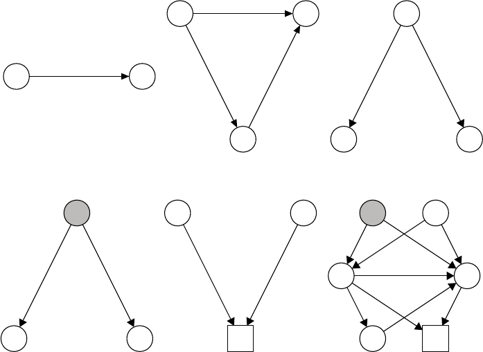
data exacerbate many of the problems of small data. As illustrated in Figure 20.1, there
are many sources of association between two variables, including direct effects, indirect
effects, measured confounding, unmeasured confounding, and selection bias [6]. Methods to
delineate causation from correlation are perhaps more pressing now than ever [7,8].
AY
(a)
A
Z
Y
(b)
W
AY
(c)
U
AY
(d)
A
C
Y
(e)
U
W
A
ZC
Y
(f)
FIGURE 20.1
Some of the sources of dependence between an exposure A and an outcome Y :(a)the
exposure A directly affects the outcome Y ; (b) the exposure A directly affects the outcome
Y as well as indirectly affects it through the mediator Z;(c)theexposureA has no effect
on the outcome Y , but an association is induced by a measured common cause W ;(d)the
exposure A has no effect on the outcome Y , but an association is induced by an unmeasured
common cause U;(e)theexposureA has no effect on the outcome Y , but an association
is induced by only examining data among those not censored C; (f) all these sources of
dependence are present. Please note this is not an exhaustive list.

Tutorial for Causal Inference 363
20.2 The Scientific Question
The first step in the causal “roadmap” is to specify the scientific objective. As a running
example, we will consider the timing of antiretroviral therapy (ART) initiation and its
impact on outcomes among HIV+ individuals. Early ART initiation has been been shown to
improve patient outcomes as well as reduce transmission between discordant couples [9,10].
Suppose we want to learn the effect of immediate ART initiation (i.e., irrespective of CD4+
T-cell count) on mortality. Large consortiums, such as the International Epidemiologic
Databases to Evaluate AIDS and Sustainable East Africa Research in Community Health,
are providing unprecedented quantities of data to answer this and other questions [12,13].
To sharply frame our scientific aim, we need to further specify the system, including the
target population (e.g., patients and context), the exposure (e.g., criteria and timing), and
the outcome. As a second try, consider our goal as learning the impact of initiating ART
within 1 month of diagnosis on 5-year all-cause mortality among adults, recently diagnosed
with HIV in Sub-Saharan Africa. This might seem like an insurmountable task, and it may
seem safer to frame our question in terms of an association. Indeed, there seems to be a
tendency to shy away from causal language when stating the scientific objective. However,
we are not fundamentally interested in the correlation between early ART initiation and
mortality among HIV+ adults. Instead, we want to isolate the effect of interest from the
spurious sources of dependence (e.g., confounding, selection bias, informative censoring) as
shown in Figure 20.1. The framework, discussed in this chapter, provides a pathway from
our scientific aim to estimation of a statistical parameter that best approximates our causal
effect, while keeping any assumptions transparent.
20.3 The Causal Model
The second step of the roadmap is to specify our causal model. Causal inference is distinct
from statistics in that it requires something more than a sample from the observed data
distribution. In particular, causal inference requires specification of background knowledge,
and causal models provide a rigorous language for expressing this knowledge and its limits.
In this chapter, we focus on structural causal models [14] to formally represent which
variables potentially affect one another, the roles of unmeasured factors, and the functional
form of those relationships. Structural causal models unify causal graphs [15], structural
equations [16,17], and counterfactuals. We also briefly introduce the Neyman–Rubin
potential outcomes framework [18–20] and discuss its relation to the structural causal model.
Consider again our running example. Let W denote the set of baseline covariates,
including sociodemographics, clinical measurements, and social constructs. The exposure
A is an indicator, equalling 1 if the patient initiated ART within 1 month of diagnosis and
equalling 0 otherwise (i.e., initiation took longer than 1 month). Finally, the outcome Y is an
indicator that the patient did not survive 5 years of follow-up. These factors have scientific
meaning to the question and comprise the set of endogenous variables: X = {W, A, Y }.They
can be measurable (e.g., age and sex) or unmeasurable and are affected by other variables
in the model.
Each endogenous variable is associated with a set of background factors U =
(U
W
,U
A
,U
Y
) with some joint distribution P
U
. These represent all the unmeasured factors,
affecting other variables in the model but not included in X. For example, U
A
could include
unknown clinic-level factors, influencing whether or not a patient initiates early ART.
364 Handbook of Big Data
Likewise, U
Y
may include a patient’s genetic risk profile. Furthermore, there might be
shared unmeasured causes between the endogenous variables. For example, socioeconomic
status may impact whether a patient initiates early ART as well as his/her 5-year
mortality.
Each endogenous variable is also associated with a structural equation. These functions
help encode our causal knowledge. Suppose, for example, we believe that the set of baseline
covariates possibly impact whether a patient initiates early ART, and that both the
covariates and the exposure may affect subsequent morality. Then we write each endogenous
variable as a deterministic function of its “parents,” variables that may impact its value:
W = f
W
(U
W
)
A = f
A
(W, U
A
)
Y = f
Y
(W, A, U
Y
). (20.1)
These functions F = {f
W
,f
A
,f
Y
} are left unspecified (nonparametric). For example, the
third equation f
Y
encodes that the covariates W and the exposure A may have influenced
the value taken by the outcome Y . We have not, however, restricted their relationships: A
and any member of W may interact on an additive (or any other) scale to affect Y and the
impacts of A and W on Y may be nonlinear.
The structural causal model, denoted M
F
, is defined by all possible distributions of P
U
and all possible sets of functions F , which are compatible with our assumptions (if any). For
the above example, there is some true joint distribution P
U,0
of health care access, personal
preferences for ART use, socioeconomic factors, etc. Randomly sampling a patient from the
population corresponds to drawing a particular realization u from P
U,0
. Likewise, there are
some true structural equations F
0
that would deterministically generate the endogenous
variables X = x if given input U = u. For a given distribution P
U
and set of functions F ,
the structural causal model M
F
describes the following data generating process for (U, X):
1. Drawing the background factors U from some joint probability distribution P
U
2. Generating the baseline covariates W as some deterministic function f
W
of U
W
3. Generating the exposure A as some deterministic function f
A
of covariates W
and U
A
4. Generating the outcome Y as some deterministic function f
Y
of covariates W ,
the exposure A,andU
Y
Thus, the model M
F
is the collection of all possible probability distributions P
U,X
for the
exogenous and endogenous variables (U, X). The true joint distribution is an element of the
causal model: P
U,X,0
∈M
F
. The structural causal model is also sometimes also called a
nonparametric structural equation model [14,21].
In other settings, we may have more in-depth knowledge about the data generating
process. This knowledge is generally encoded in two ways. First, excluding a variable from
the parent set of X
j
encodes that this variable does not directly impact the value X
j
takes.
These assumptions are known as exclusion restrictions. Second, restricting the set of allowed
distributions for P
U
encodes that some variables do not have any unmeasured common
causes. These assumptions are known as independence assumptions. Suppose, for example,
that patients were randomized R to early ART initiation, but adherence A was imperfect.
Then the treatment assignment R would only be determined by chance (e.g., a coin flip) and
not influenced by the baseline covariates W . The unmeasured factors determining treatment
assignment would be independent from all other unmeasured factors:
U
R
|=
(U
W
,U
A
,U
Y
).

Tutorial for Causal Inference 365
This is an independence assumption that restricts the allowed distribution of background
factors P
U
. Furthermore, suppose that randomization R only affects the mortality Y through
its effect on adherence A. The resulting structural equations are then
W = f
W
(U
W
)
R = f
R
(U
R
)
A = f
A
(W, R, U
A
)
Y = f
Y
(W, A, U
Y
). (20.2)
We have made two exclusion restrictions: (1) the baseline covariates W do not influence
randomization R and (2) randomization R has no direct effect on the outcome Y .The
structural causal model is then defined by all probability distributions for U that are com-
patible with our independence assumptions and all sets of functions F =(f
W
,f
R
,f
A
,f
Y
)
that are compatible with our exclusion restrictions.
A causal graph can be drawn from the structural causal model [14]. Each endogenous
variable (node) is connected to its parents and background error term with a directed arrow.
The potential dependence between the background factors is encoded by the inclusion of
a node representing any unmeasured common cause. Exclusion restrictions are encoded
by absence of a directed arrow. Likewise, independence assumptions are encoded with the
absence of a node representing an unmeasured common cause. The corresponding causal
graphs for the two examples are given in Figure 20.2.
U
W
AY
(a) (b)
U
W
AY
R
FIGURE 20.2
Directed acyclic graphs representing the structural causal model for our study (Equa-
tion 20.1) and for the hypothetical randomized trial (Equation 20.2). (a) This graph
only encodes the time ordering between baseline covariates W ,theexposureA,andthe
outcome Y . A single node U represents the unmeasured common causes of the endogenous
variables. (b) This graph encodes the randomization R of some treatment with incomplete
adherence A. There are two exclusion restrictions: The baseline covariates W do not impact
the randomization R, and the randomization R has no direct effect on the outcome Y .There
is also an independence assumption: the unmeasured factors contributing to randomization
are independent of the unmeasured factors, contributing to the other variables.
..................Content has been hidden....................
You can't read the all page of ebook, please click here login for view all page.