
Tutorial for Causal Inference 371
associations (i.e., conditioning on a collider). The rationale for condition 2 is to block
any remaining spurious sources of association. For the basic structure (Figure 20.3),
the randomization assumption will hold if the following independence assumptions are
true:
U
A
|=
U
Y
and U
A
|=
U
W
or U
Y
|=
U
W
.
There must not be any unmeasured common causes of the exposure and the outcome, and of
the exposure and covariates or of the outcome and covariates. As illustrated in Figure 20.4,
this graphical criteria can aid in the selection of an appropriate adjustment set.
When the randomization assumption holds, we can identify the distribution of counter-
factuals within strata of covariates. Specifically, we have that for each P
U,X
∈M
F
P
U,X
(Y
a
= y|W = w )=P
U,X
(Y
a
= y|A = a, W = w)
= P (Y = y|A = a, W = w),
where the distribution P of the observed data is implied by P
U,X
. This gives us the G-
computation identifiability result [27] for the true distributions P
U,X,0
and P
0
:
E
U,X,0
(Y
a
)=
w
E
0
(Y |A = a, W = w)P
0
(W = w),
where the summation generalizes to an integral for continuous covariates. Likewise, we can
identify the difference in the expected counterfactual outcomes (i.e., the average treatment
effect) in terms of the difference in the conditional mean outcomes, averaged with respect
to the covariate distribution:
E
U,X,0
(Y
1
− Y
0
)
Ψ
F
(P
U,X,0
)
=
w
E
0
(Y |A =1,W = w) − E
0
(Y |A =0,W = w)
P
0
(W = w)
Ψ(P
0
)
.
Identifiability also relies on having sufficient support in the data. The G-computation
formula requires that the conditional mean E
0
(Y |A = a, W = w) is well defined for all
possible values of w and levels of a of interest. In a nonparametric statistical model, each
exposure of interest must occur with some positive probability for each possible covariate
stratum:
min
a∈A
P
0
(A = a|W = w) > 0, for all w for which P
0
(W = w) > 0.
This condition is known as the positivity assumption and as the experimental treatment
assignment assumption.
Suppose, for example, that the randomization assumption holds conditionally on a single
binary baseline covariate. Then our statistical estimand could be rewritten as
Ψ(P
0
)=
E
0
(Y |A =1,W =1)− E
0
(Y |A =0,W =1)
P
0
(W =1)
+
E
0
(Y |A =1,W =0)− E
0
(Y |A =0,W =0)
P
0
(W =0).
As an extreme, suppose that in the population, there are zero exposed patients with this
covariate: P
0
(A =1|W = 1) = 0. Then there would be no information about outcomes under
the exposure for this subpopulation. To identify the treatment effect, we could consider a
different target parameter (e.g., the effect among those with W = 0) or consider additional
modeling assumptions (e.g., the effect is the same among those with W =1andW =0).
372 Handbook of Big Data
Both options are a bit dissatisfying and other approaches may be taken [37]. The risk of
violating the positivity assumption is exacerbated with higher dimensional data (i.e., as the
number of covariates or their levels grow).
In many cases, our initial assumptions, encoded in the structural causal model M
F
,
are not sufficient to identify the causal effect Ψ
F
(P
U,X
). Indeed, for our running example
(Figure 20.2a), the set of baseline covariates is not sufficient to block the back-door
paths from the outcome to the exposure. The question then becomes how to proceed?
Possible options include giving up, gathering more data, or continuing to estimation while
clearly acknowledging the lack of identifiability during the interpretation step. To facilitate
the third option, we can use M
F∗
to denote the structural causal model, augmented
with additional convenience-based assumptions needed for identifiability. This gives us a
way to proceed, while separating our real knowledge M
F
from our wished identifiability
assumptions M
F∗
.
Overall, identifiability assumptions and resulting estimands are specific to the causal
parameter Ψ
F
(P
U,X
). We are focusing on a point treatment effect (i.e., distribution of
counterfactuals under interventions on a single node or variable). Different identifiability
results are needed for interventions on more than one node (e.g., longitudinal treatment
effects and direct effects) and interventions responding to patient characteristics (e.g.,
dynamic regimes). Furthermore, a given causal parameter may have more than one
identifiability result (e.g., instrumental variables and the front-door criterion). See, for
example, Pearl [14].
Common Pitfall: Stating vs. Evaluating the Identifiability Assumptions
There is a temptation to simply state the identifiability assumptions and proceed
to the analysis. The identifiability assumptions require careful consideration. Directed
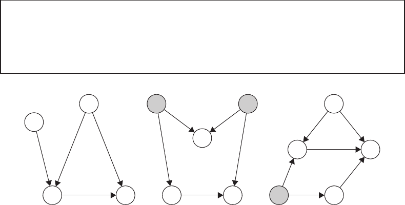
W2
AY
W1
(a)
W
AY
UU*
(b)
W
A
U
L
Y
(c)
FIGURE 20.4
Considering the back-door criterion. (a) The set of covariates W 2 is sufficient to block the
back-door path from Y → W 2 → A. Therefore, the randomization assumption will hold
conditionally on W 2. Further adjustment for W 1 is unnecessary and potentially harmful. (b)
The randomization assumption holds conditionally on ∅. Adjusting for W (i.e., conditioning
on a collider of U and U
∗
) opens a back-door path and induces a spurious association
between A and Y . (c) The randomization assumption holds conditionally on (W, L). The
covariates L are needed to block the back-door path from Y → L → U → A, even though
L occurs temporally after the exposure A.

Tutorial for Causal Inference 373
acyclic graphs facilitate the evaluation of assumptions by subject-matter experts
without extensive statistical training. When interpreting the analysis, any convenience-
based causal assumptions should be transparently stated and explained.
20.7 Estimation and Inference
In the previous step, we defined the parameter of interest as a mapping from the statistical
model to the parameter space: Ψ : M→R. In other words, the statistical parameter is
a function, whose input is any distribution P compatible with the statistical model and
whose output is a real number. The parameter mapping applied to the true observed data
distribution P
0
is called the estimand and denoted Ψ(P
0
). Recall we have n independent,
identically distributed (i.i.d.) copies of the random variable O =(W, A, Y ). The empirical
distribution P
n
corresponds to putting a weight 1/n on each copy of O
i
.Anestimator is a
function, whose input is the observed data (a realization of P
n
) and output a value in the
parameter space.
In this chapter, we consider substitution estimators based on the G-computation
identifiability result [27]:
Ψ(P
0
)=E
0
E
0
(Y |A =1,W) − E
0
(Y |A =0,W)
. (20.3)
A simple substitution estimator for Ψ(P
0
) can be implemented as follows:
1. Estimate the conditional expectation of the outcome, given the exposure and
covariates, denoted
ˆ
E(Y |A, W ).
2. Use this estimate to generate the predicted outcomes for each unit, setting A =1
and A =0.
3. Take the sample average of the difference in these predicted outcomes:
ˆ
Ψ(P
n
)=
1
n
n
i=1
ˆ
E(Y
i
|A
i
=1,W
i
) −
ˆ
E(Y
i
|A
i
=0,W
i
).
The last step corresponds to estimating the marginal covariate distribution P
0
(W )withthe
sample proportion:
1
n
i
I(W
i
= w).
There are many options available for estimating the conditional expectation E
0
(Y |A, W ).
Often, parametric models are used to relate the conditional mean outcome to the possible
predictor variables and the exposure. Suppose, for example, we knew that the conditional
expectation of a continuous outcome could be described by the following parametric
model:
E
0
(Y |A, W )=β
0
+ β
1
A + β
2
W
1
+ β
3
W
2
+ β
4
A
∗
W
1
+ β
5
A
∗
W
2
,
where W = {W
1
,W
2
} denotes the set of covariates, needed for identifiability. Then
this knowledge should have been encoded in our structural causal model M
F
with
implied restrictions on our statistical model M. (In other words, we avoid introducing
new assumptions during the analysis.) The coefficients in this regression model could be
estimated with maximum likelihood or with ordinary least squares regression. The estimate
ˆ
β
1
does not, however, provide an estimate of the G-computation identifiability result. The

374 Handbook of Big Data
exact interpretation of
ˆ
β
1
depends on which variables and which interactions are included
in the parametric model. To obtain an estimate of Ψ(P
0
), we need to average the predicted
outcomes with respect to the distribution of covariates:
ˆ
Ψ(P
n
)=
1
n
n
i=1
ˆ
E(Y
i
|A
i
=1,W
i
) −
ˆ
E(Y
i
|A
i
=0,W
i
)
=
1
n
n
i=1
ˆ
β
1
+
ˆ
β
4
W
1,i
+
ˆ
β
5
W
2,i
.
As a second example, suppose we knew that the conditional risk of a binary outcome could
be described by the following parametric model:
logit
E
0
(Y|A, W)
= β
0
+ β
1
A+β
2
W
1
+ ···+ β
11
W
10
,
where W = {W
1
...,W
10
} denotes the set of covariates, needed for identifiability. Then
the estimate
ˆ
β
1
would provide an estimate of the logarithm of the conditional odds ratio.
An estimate of the G-computation identifiability result is given by averaging the expected
outcomes under the exposure A = 1 and control A =0:
ˆ
Ψ(P
n
)=
1
n
n
i=1
1
1+exp
−(
ˆ
β
0
+
ˆ
β
1
+
ˆ
β
2
W
1,i
+···+
ˆ
β
11
W
10,i
)
−
1
1+exp
−(
ˆ
β
0
+
ˆ
β
2
W
1,i
+···+
ˆ
β
11
W
10,i
)
.
In most cases, our background knowledge is inadequate to describe the conditional
expectation E
0
(Y |A, W )withsuchparametricmodels.Indeed, with high dimensional data,
the sheer number of potential covariates will likely make it impossible to correctly specify the
functional form. If the assumed parametric model is incorrect, the point estimates will often
be biased and inference misleading. In other words, the structural causal model M
F
,repre-
senting our knowledge of the underlying data generating process, often implies a nonpara-
metric statistical model M. Our estimation approach should respect the statistical model.
To avoid unsubstantiated assumptions about functional form, it is sometimes possible
to estimate E
0
(Y |A, W ) with the empirical mean in each exposure–covariate stratum.
Unfortunately, even when all covariates are discrete valued, nonparametric maximum
likelihood estimators quickly become ill-defined due to the curse of dimensionality; the
number of possible exposure–covariate combinations far exceeds the number of observations.
Again, this problem becomes exacerbated with big data, where, for example, there are
hundreds of potential covariates under consideration.
Various model selection routines can help alleviate these problems. For example, stepwise
regression will add and subtract variables in hopes of minimizing the Akaike information
criterion or the Bayesian information criterion. Other data-adaptive methods, based on
cross-validation, involve splitting the data into training and validation sets. Each possible
algorithm (e.g., various parametric models or semiparametric methods) is then fit on the
training set and its performance assessed on the validation set. The measure of performance
can be defined by a loss function, such as the L2-squared error or the negative log likelihood.
Super learner, for example, uses cross-validation to select the candidate algorithm with the
best performance or to build the optimal (convex) combination of estimates from candidate
algorithms [38,39]. (For further details, see Chapter 19.) A point estimate could then be
obtained by averaging the difference in predicted outcomes for each unit under the exposure
and under the control.
Although these data-adaptive methods avoid betting on one apriorispecified parametric
regression model and are amenable to semiparametric algorithms, there is no reliable
Tutorial for Causal Inference 375
way to obtain statistical inference for parameters, such as the G-computation estimand
Ψ(P
0
). Treating the final algorithm as if it were prespecified ignores the selection process.
Furthermore, the selected algorithm was tailored to maximize/minimize some criterion
with regard to the conditional expectation E
0
(Y |A, W ) and will, in general, not provide
the best bias–variance trade-off for estimating the statistical parameter Ψ(P
0
). Indeed,
estimating the conditional mean outcome Y in every stratum of (A, W )isamuch
more ambitious task than estimating one number (the difference in conditional means,
averaged with respect to the covariate distribution). Thus, without an additional step, the
resulting estimator will be overly biased relative to its standard error, preventing accurate
inference.
Targeted maximum likelihood estimation (TMLE) provides a way forward [3,40]. TMLE
is a general algorithm for the construction of double robust, semiparametric, efficient
substitution estimators. TMLE allows for data-adaptive estimation while obtaining valid
statistical inference. The algorithm is detailed in Chapter 22. Although TMLE is a
general algorithm for a wide range of parameters, we focus on its implementation for the
G-computation estimand. Briefly, the TMLE algorithm uses information in the estimated
exposure mechanism
ˆ
P (A|W ) to update the initial estimator of the conditional mean
E
0
(Y |A, W ). The targeted estimates are then substituted into the parameter mapping.
The updating step achieves a targeted bias reduction for the parameter of interest Ψ(P
0
)
and serves to solve the efficient score equation. As a result, TMLE is a double robust
estimator; it will be consistent for Ψ(P
0
) is either the conditional expectation E
0
(Y |A, W )
or the exposure mechanism P
0
(A|W ) is estimated consistently. When both functions are
consistently estimated at a fast enough rate, the TMLE will be efficient in that it achieves the
lowest asymptotic variance among a large class of estimators. These asymptotic properties
typically translate into lower bias and variance in finite samples. The advantages of TMLE
have been repeatedly demonstrated in both simulation studies and applied analyses [37,41–
43]. The procedure is available with standard software such as the tmle and ltmle packages
in R [44–46].
Thus far, we have discussed obtaining a point estimate from a simple or targeted substi-
tution estimator. To create confidence intervals and test hypotheses, we also need to quantify
uncertainty. A simple substitution estimator based on a correctly specified parametric model
is asymptotically linear, and its variance can be approximated by the variance of its influence
curve, divided by sample size n. It is worth emphasizing that our estimand Ψ(P
0
) often does
not correspond to a single coefficient, and therefore we usually cannot read off the reported
standard error from common software. Under reasonable conditions, the TMLE is also
asymptotically linear and inference can be based on an estimate of its influence curve.
Overall, this chapter focused on substitution estimators (simple and targeted) of the
G-computation identifiability result [27]. The simple substitution estimator only requires
an estimate of the marginal distribution of baseline covariates P
0
(W ) and the conditional
expectation of the outcome, given the exposure and covariates E
0
(Y |A, W ). TMLE also
requires an estimate of the exposure mechanism P
0
(A|W ). There are many other algorithms
available for estimation of Ψ(P
0
). A popular class of estimators relies only on estimation
of the exposure mechanism [47–49]. Inverse probability of treatment weighting (IPTW)
estimators, for example, control for measured confounders by up-weighting exposure–
covariate groups that are underrepresented and down-weighting exposure–covariate groups
that are overrepresented (relative to what would be seen were the exposure randomized).
Its double robust counterpart, augmented-IPTW, shares many of the same properties as
TMLE [50,51]. A key distinction is that IPTW and augmented-IPTW are solutions to
estimating equations and therefore respond differently in the face of challenges due to strong
confounding and rare outcomes [37,52]. Throughout, we maintain that estimators should
..................Content has been hidden....................
You can't read the all page of ebook, please click here login for view all page.