From the world cloud, it is clear that there are still numbers and words that are not relevant for us. For example, there is the technical term package, and we can remove those. In addition to that, showing plural versions of nouns is redundant. Let's use the removeNumbers function to remove numbers:

> v <- tm_map(v, removeNumbers)

In order to remove some frequent domain-specific words with less relevance to our purpose, we need to see most common words in our corpus. To do that, we can compute TermDocumentMatrix, as shown in the following snippet:

> tdm <- TermDocumentMatrix(v)

The tdm object is a matrix that holds the words in the rows and the documents in the columns, where the cells show the number of occurrences. For example, let's take a look at the first 10 words' occurrences in the first 25 documents:

> inspect(tdm[1:10, 1:25])
<<TermDocumentMatrix (terms: 10, documents: 25)>>
Non-/sparse entries: 10/240
Sparsity : 96%
Maximal term length: 10
Weighting : term frequency (tf)
Sample :
 Docs
Terms 1 10 2 3 4 5 6 7 8 9
 abbyy 0 0 1 0 0 0 0 0 0 0
 access 0 0 1 0 0 0 0 0 0 0
 accessible 1 0 0 0 0 0 0 0 0 0
 accurate 1 0 0 0 0 0 0 0 0 0
 adaptable 1 0 0 0 0 0 0 0 0 0
 api 0 0 1 0 0 0 0 0 0 0
 error 1 0 0 0 0 0 0 0 0 0
 metrics 1 0 0 0 0 0 0 0 0 0
 models 1 0 0 0 0 0 0 0 0 0
 predictive 1 0 0 0 0 0 0 0 0 0

Now, we can extract the overall number of occurrences for each word using the findFrequentTerms function. Let's show all the terms that show up in the descriptions at least 100 times:

> findFreqTerms(tdm, lowfreq = 100)
[1] "models" "api" "bayesian" "tools"
[5] "data" "analysis" "based" "package"
[9] "implementation" "optimization" "model" "random"
[13] "via" "the" "files" "visualization"
[17] "modelling" "multivariate" "networks" "detection"
[21] "time" "regression" "gene" "series"
[25] "functions" "sampling" "prediction" "sparse"
[29] "algorithm" "using" "multiple" "dynamic"
[33] "distributions" "method" "estimation" "linear"
[37] "matrix" "robust" "testing" "statistics"
[41] "classification" "methods" "tests" "mixture"
[45] "generalized" "simulation" "learning" "survival"
[49] "test" "graphical" "interface" "selection"
[53] "spatial" "inference" "clustering" "fast"
[57] "statistical" "function" "sets" "modeling"
[61] "distribution" "plots" "client" "mixed"
[65] "network" "nonparametric" "likelihood" "variable"

From the preceding list, we can see that there are some terms that are not relevant for us. If we want to get rid of them, we can construct our own stop words. Say we do not find the package, the, via, using, or based words because they are irrelevant for our purpose:

> myStopwords <- c('the', 'via', 'package', 'based', 'using')

Now, let's remove these words from our corpus:

> v <- tm_map(v, removeWords, myStopwords)

Now, let's remove the plural forms of the nouns. For this purpose, we can use stemming algorithms. 

The text documents always use different forms of a word in order to build a coherent meaning of the text. In the process of doing so, a word can take several forms, for example, send, sent, sending, sends. In addition to this type of form, there are sets of derivationally-related terms that have analogous meanings, such as democracy, democratic, and democratization. It would be more meaningful if search engines recognize these forms of the words, and return the documents that contain another form of the same word. In order to achieve that, we are going to use one of the libraries, called the Snowballc package. If the library does not exist, we know how to install it, don't we? 

wordStem supports different languages and can identify the stem of a character vector. Let's check some of the examples:

> wordStem(c('dogs', 'walk', 'print', 'printed', 'printer', 'printing'))
[1] "dog" "walk" "print" "print" "printer" "print"

Copy the words from the already-existing corpus into another object:

> d <- v

Then stem all the words in the documents:

> v <- tm_map(v, stemDocument, language = "english")

Here, we called the stemDocument function, which is the wrapper around the Snowballc package's wordStem function. Now, let's call the stemCompletion function on our copied directory. Here, we have to write out our own function. The idea is to split each document into words by a space, apply the stemCompletion function, and then concatenate the words into sentences again:

> stemCompletion2 <- function(x, dictionary) {
  x <- unlist(strsplit(as.character(x), " "))
  x <- x[x != ""]
  x <- stemCompletion(x, dictionary=dictionary)
  x <- paste(x, sep="", collapse=" ")
  PlainTextDocument(stripWhitespace(x))
}

Now, let's run the function as follows:

> v <- lapply(v, stemCompletion2, dictionary=d)

This step is going to use CPU for around 30-60 minutes, so you can either step this process or wait until this is done. Run the following command to convert into VCorpus:

> v <- Corpus(VectorSource(v))
> tdm <- TermDocumentMatrix(v)
> findFreqTerms(tdm, lowfreq = 100)
  [1] "118" "164" "access" "author"
  [5] "character" "content" "datetimestamp" "description"
  [9] "heading" "hour" "isdst" "language"
 [13] "list" "mday" "meta" "min"
 [17] "model" "mon" "origin" "predict"
 [21] "sec" "wday" "yday" "year"
 [25] "api" "bayesian" "computation" "tool"
 [29] "data" "analysing" "implement" "optim"
 [33] "estimability" "random" "analyse" "file"
 [37] "visual" "associate" "use" "multivariable"
 [41] "network" "measure" "popular" "detect"
 [45] "simulate" "time" "fit" "regression"
 [49] "gene" "infer" "serial" "function"
 [53] "process" "valuation" "sample" "plot"
 [57] "sparse" "response" "algorithm" "design"
 [61] "multiplate" "select" "dynamic" "distributed"
 [65] "method" "effect" "linear" "matrix"
 [69] "robust" "test" "map" "statistic"
 [73] "classifcation" "read" "applicable" "mixture"
 [77] "general" "learn" "survival" "graphic"
 [81] "interface" "densities" "genetic" "spatial"
 [85] "calculate" "cluster" "fast" "informatic"
 [89] "studies" "object" "equating" "curvature"
 [93] "variable" "set" "dataset" "utilities"
 [97] "generate" "create" "database" "interact"
[101] "client" "mixed" "weight" "analyze"
[105] "system" "nonparametric" "structural" "tablature"
[109] "likelihood" "tree" "libraries" "correlated"
[113] "interva" "covariable"

Let's check the density of the document term matrix:

> tdm<<TermDocumentMatrix (terms: 20202, documents: 12658)>>
Non-/sparse entries: 339239/255377677
Sparsity : 100%
Maximal term length: 33
Weighting : term frequency (tf)

As we can see, the density has increased. However, we can see there are still some terms we do not want in our corpus. We can refine further until we reach our desired results. 

In addition to these results, we can build TermDocumentMatrix:

> dtm <- TermDocumentMatrix(v)
> m <- as.matrix(dtm) 
> v <- sort(rowSums(m),decreasing=TRUE) 
> d <- data.frame(word = names(v),freq=v) 
> head(d, 10)
 word freq
character character 75961
list      list      38009
language  language  12697
description description 12686
meta       meta      12668
content    content   12667
origin     origin    12663
year       year      12662
min        min       12660
sec        sec       12659

We can use the RColorBrewer library to color our graph:

### Load the package or install if not present
if (!require("RColorBrewer")) {
  install.packages("RColorBrewer")
  library(RColorBrewer)
}

And finally:

> set.seed(1234)
> wordcloud::wordcloud(words = d$word, freq = d$freq, min.freq = 1,
+ max.words=200, random.order=FALSE, rot.per=0.35,
+ colors=brewer.pal(8, "Dark2"))

The output of the preceding snippet should generate the color-coded cloud model, similar to this:

If you want to plot a bar chart of the first 10 most frequent words, it can be plotted using the following code: 

> barplot(d[1:10,]$freq, las = 2, names.arg = d[1:10,]$word,
+ col ="lightblue", main ="Most frequent words",
+ ylab = "Word frequencies")

Running the preceding command should produce the following graph:

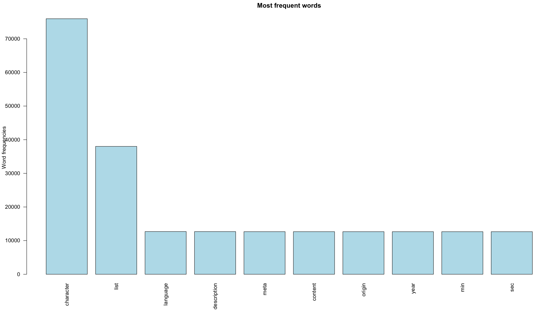
The graph shows that the most frequent words are character, list, language, description, meta, content, origin, and year.