

Planning storage pools
This chapter describes considerations for planning storage pools for an IBM FlashSystem implementation. It explains various pool configuration options, including Easy Tier and data reduction pools (DRPs). It provides and provides best practices on implementation and an overview of some typical operations with MDisks.
This chapter includes the following topics:
4.1 Introduction to pools
In general, a storage pool or pool, sometimes referred to as managed disk group, is a grouping of storage capacity that is used to provision volumes and logical units (LUNs) that can subsequently be made visible to hosts.
IBM FlashSystem supports the following types of pools:
•Standard pools: Parent pools and child pools
•DRPs: Parent pools and quotaless child pools
Standard pools were available since the initial release of IBM Spectrum Virtualize in 2003 and can include fully allocated or thin-provisioned volumes.
Real-time Compression (RtC) is allowed only with standard pools on some older IBM SAN Volume Controller hardware models and should not be implemented in new configurations.
|
Note: The latest node hardware does not support RtC.
SA2 and SV2 IBM SAN Volume Controller node hardware do not support the use of RtC volumes. To migrate a system to use these node types, all RtC volumes must be removed (migrated) to uncompressed standard pool volumes, or into a DRP.
|
IBM FlashSystems that use standard pools cannot be configured by using RtC.
DRPs represent a significant enhancement to the storage pool concept because the virtualization layer is primarily a simple layer that runs the task of lookups between virtual and physical extents. With the introduction of data reduction technology, compression, and deduplication, it has become more of a requirement to have an uncomplicated way to stay thin.
DRPs increase infrastructure capacity usage by employing new efficiency functions and reducing storage costs. The pools enable you to automatically de-allocate (not to be confused with deduplicate) and reclaim capacity of thin-provisioned volumes containing deleted data. In addition, for the first time, the pools enable this reclaimed capacity to be reused by other volumes.
Either pool type can be made up of different tiers. A tier defines a performance characteristic of that subset of capacity in the pool. Often, no more than three tier types are be defined in a pool (fastest, average, and slowest). The tiers and their usage are managed automatically by the Easy Tier function.
4.1.1 Standard pool
Standard pools (also referred to as traditional storage pools), provide a way of providing storage in IBM FlashSystem. They use a fixed allocation unit of an extent. Standard pools are still a valid method to providing capacity to hosts. For more information about guidelines for implementing standard pools, see 4.2, “Storage pool planning considerations” on page 132.
IBM FlashSystem can define parent and child pools. A parent pool has all the capabilities and functions of a normal IBM FlashSystem pool. A child pool is a logical subdivision of a storage pool or managed disk group. Like a parent pool, a child pool supports volume creation and migration.
When you create a child pool in a standard parent pool the user must specify a capacity limit for the child pool. This limit allows for a quota of capacity to be allocated to the child pool. This capacity is reserved for the child pool and detracts from the available capacity in the parent pool. This process is different than the method with which child pools are implemented in a DRP. For more information, see “Quotaless data reduction child pool” on page 118.
A child pool inherits its tier setting from the parent pool. Changes to a parent’s tier setting are inherited by child pools.
A child pool supports the Easy Tier function if Easy Tier is enabled on the parent pool. The child pool also inherits Easy Tier status, pool status, capacity information, and back-end storage information. The I/O activity of parent pool is the sum of the I/O activity of itself and the child pools.
Parent pools
Parent pools receive their capacity from MDisks. To track the space that is available on an MDisk, the system divides each MDisk into chunks of equal size. These chunks are called extents and are indexed internally. The choice of extent size affects the total amount of storage that is managed by the system. The extent size remains constant throughout the lifetime of the parent pool.
All MDisks in a pool are split into extents of the same size. Volumes are created from the extents that are available in the pool. You can add MDisks to a pool at any time to increase the number of extents that are available for new volume copies or to expand volume copies. The system automatically balances volume extents between the MDisks to provide the best performance to the volumes.
You cannot use the volume migration functions to migrate volumes between parent pools that feature different extent sizes. However, you can use volume mirroring to move data to a parent pool that has a different extent size.
Choose extent size wisely according to your future needs. A small extent size limit your overall usable capacity, but a larger extent size can waste storage. For example, if you select an extent size of 8 GiB, but then only create a 6 GiB volume, one entire extent is allocated to this volume (8 GiB) and hence 2 GiB are unused.
When you create or manage a parent pool, consider the following general guidelines:
•Ensure that all MDisks that are allocated to the same tier of a parent pool are the same RAID type. This configuration ensures that the same resiliency is maintained across that tier. Similarly, for performance reasons, do not mix RAID types within a tier. The performance of all volumes is reduced to the lowest achiever in the tier and a mismatch of tier members can result in I/O convoying effects where everything is waiting on the slowest member.
•An MDisk can be associated with only one parent pool.
•You should specify a warning capacity for a pool. A warning event is generated when the amount of space that is used in the pool exceeds the warning capacity. The warning threshold is especially useful with thin-provisioned volumes that are configured to automatically use space from the pool.
•Volumes are associated with just one pool, except for the duration of any migration between parent pools.
•Volumes that are allocated from a parent pool are by default striped across all the storage that is placed into that parent pool. Wide striping can provide performance benefits.
•You can only add MDisks that are in unmanaged mode to a parent pool. When MDisks are added to a parent pool, their mode changes from unmanaged to managed.
•You can delete MDisks from a parent pool under the following conditions:
– Volumes are not using any of the extents that are on the MDisk.
– Enough free extents are available elsewhere in the pool to move extents that are in use from this MDisk.
– The system ensures that all extents that are used by volumes in the child pool are migrated to other MDisks in the parent pool to ensure that data is not lost.
|
Important: Before you remove MDisks from a parent pool, ensure that the parent pool has enough capacity for child pools that are associated with the parent pool.
|
•If the parent pool is deleted, you cannot recover the mapping that existed between extents that are in the pool or the extents that the volumes use. If the parent pool includes associated child pools, you must delete the child pools first and return its extents to the parent pool. After the child pools are deleted, you can delete the parent pool. The MDisks that were in the parent pool are returned to unmanaged mode and can be added to other parent pools. Because the deletion of a parent pool can cause a loss of data, you must force the deletion if volumes are associated with it.
|
Note: Deleting a child or parent pool is unrecoverable.
If you force-delete a pool, all volumes in that pool are deleted, even if they are mapped to a host and are still in use. Use extreme caution when force-deleting pool objects because volume-to-extent mapping cannot be recovered after the delete is processed.
Force-deleting a storage pool is possible only with the command line tools. See the rmmdiskgrp command-help for details.
|
•When you delete a pool with mirrored volumes, consider the following points:
– if the volume is mirrored and the synchronized copies of the volume are all in the same pool, the mirrored volume is destroyed when the storage pool is deleted.
– If the volume is mirrored and a synchronized copy exists in a different pool, the volume remains after the pool is deleted.
You might not be able to delete a pool or child pool if Volume Delete Protection is enabled. In code versions 8.3.1 and later, Volume Delete Protection is enabled by default. However, the granularity of protection is improved; you can now specify Volume Delete Protection to be enabled or disabled on a per-pool basis, rather than on a system basis as was previously the case.
Child pools
Instead of being created directly from MDisks, child pools are created from existing capacity that is allocated to a parent pool. As with parent pools, volumes can be created that specifically use the capacity that is allocated to the child pool. Child pools are similar to parent pools with similar properties and can be used for volume copy operation.
Child pools are created with fully-allocated physical capacity; that is, the physical capacity that is applied to the child pool is reserved from the parent pool, as though you created a fully-allocated volume of the same size in the parent pool.
The allocated capacity of the child pool must be smaller than the free capacity that is available to the parent pool. The allocated capacity of the child pool is no longer reported as the free space of its parent pool. Instead, the parent pool reports the entire child pool as used capacity. You must monitor the used capacity (instead of the free capacity) of the child pool instead.
When you create or work with a child pool, consider the following general guidelines:
•Child pools are created automatically by IBM Spectrum Connect VASA client to implement VMware vVols.
•As with parent pools, you can specify a warning threshold that alerts you when the capacity of the child pool is reaching its upper limit. Use this threshold to ensure that access is not lost when the capacity of the child pool is close to its allocated capacity.
•On systems with encryption enabled, child pools can be created to migrate existing volumes in a non-encrypted pool to encrypted child pools. When you create a child pool after encryption is enabled, an encryption key is created for the child pool even when the parent pool is not encrypted. You can then use volume mirroring to migrate the volumes from the non-encrypted parent pool to the encrypted child pool.
•Ensure that any child pools that are associated with a parent pool have enough capacity for the volumes that are in the child pool before removing MDisks from a parent pool. The system automatically migrates all extents that are used by volumes to other MDisks in the parent pool to ensure data is not lost.
•You cannot shrink the capacity of a child pool to less than its real capacity. The system uses reserved extents from the parent pool that use multiple extents. The system also resets the warning level when the child pool is shrunk, and issues a warning if the level is reached when the capacity is shrunk.
•The system supports migrating a copy of volumes between child pools within the same parent pool or migrating a copy of a volume between a child pool and its parent pool. Migrations between a source and target child pool with different parent pools are not supported. However, you can migrate a copy of the volume from the source child pool to its parent pool. The volume copy can then be migrated from the parent pool to the parent pool of the target child pool. Finally, the volume copy can be migrated from the target parent pool to the target child pool.
•Migrating a volume between parent and child pool (with the same encryption key or no encryption) results in a nocopy migration. That is, the data does not move. Instead, the extents are re-allocated to the child or parent pool and the accounting of the used space is corrected. That is, the free extents are reallocated to the child or parent to ensure the total capacity allocated to the child pool remains unchanged.
•A special form of quotaless data reduction child pool can be created from a data reduction parent pool. For more information, see “Quotaless data reduction child pool” on page 118
Small Computer System Interface unmap in a standard pool
A standard pool can use Small Computer System Interface (SCSI) unmap space reclamation, but not as efficiently as a DRP.
When a host submits a SCSI unmap command to a volume in a standard pool, the system changes the unmap command into a write_same command of zeros. This unmap command becomes an internal special command and can be handled accordingly by different layers in the system.
For example, the cache does not mirror the data; instead, it passes the special reference to zeros. The RtC functions reclaim those areas (assuming 32 KB or larger) and shrink the volume allocation.
The back-end layers also submit the write_same command of zeros to the internal or external MDisk devices. For a Flash or SSD-based MDisk this process results in the device freeing the capacity back to its available space. Therefore, it shrinks the used capacity on Flash or SSD, which helps to improve the efficiency of garbage collection on the device and performance. The process of reclaiming space is called garbage collection.
For Nearline SAS drives, the write_same of zeros commands can overload the drives themselves, this can result in performance problems.
|
Important: A standard pool does shrink its used space as the result of a SCSI unmap command. The backend capacity might shrink its used space, but the pool used capacity does not shrink.
The exception is with RtC volumes where the reused capacity of the volume might shrink; however, the pool allocation to that RtC volume remains unchanged. It means that an RtC volume can reuse that unmapped space first before requesting more capacity from the thin provisioning code.
|
Thin-provisioned volumes in a standard pool
A thin-provisioned volume presents a different capacity to mapped hosts than the capacity that the volume uses in the storage pool. IBM FlashSystem supports thin-provisioned volumes in standard pools.
|
Note: While DRPs fundamentally support thin-provisioned volumes, they are used in conjunction with compression and deduplication. With DRPs, you should avoid the use of thin-provisioned volumes without additional data reduction.
|
In standard pools, thin-provisioned volumes are created as a specific volume type; that is, based on capacity-savings criteria. These properties are managed at the volume level. The virtual capacity of a thin-provisioned volume is typically significantly larger than its real capacity. Each system uses the real capacity to store data that is written to the volume, and metadata that describes the thin-provisioned configuration of the volume. As more information is written to the volume, more of the real capacity is used.
The system identifies read operations to unwritten parts of the virtual capacity and returns zeros to the server without the use of any real capacity. For more information about storage system, pool, and volume capacity metrics, see Chapter 9, “Implementing a storage monitoring system” on page 387.
Thin-provisioned volumes can also help simplify server administration. Instead of assigning a volume with some capacity to an application and increasing that capacity as the needs of the application change, you can configure a volume with a large virtual capacity for the application. You can then increase or shrink the real capacity as the application needs change, without disrupting the application or server.
It is important to monitor physical capacity if you want to provide more space to your hosts than is physically available in your IBM FlashSystem. For more information about monitoring the physical capacity of your storage, and an explanation of the difference between thin provisioning and over-allocation, see 9.5, “Creating alerts for IBM Spectrum Control and IBM Storage Insights” on page 425.
Thin provisioning on top of Flash Core Modules
If you use the compression functions that are provided by the IBM Flash Core Modules (FCMs) in your FlashSystem as a mechanism to add data reduction to a standard pool while maintaining the maximum performance, take care to understand the capacity reporting, in particular if you want to thin provision on top of the FCMs.
The FCM RAID array reports its theoretical maximum capacity, which can be as large as 4:1. This capacity is the maximum that can be stored on the FCM array. However, it might not reflect the compression savings that you achieve with your data.
It is recommended that you start conservatively, especially if you are allocating this capacity to IBM SAN Volume Controller or another IBM FlashSystem (the virtualizer).
You must first understand your expected compression ratio. In an initial deployment, allocate approximately 50% fewer savings. You can easily add “volumes” to the back-end storage system to present as new external “MDisk” capacity to the virtualizer later if your compression ratio is met or bettered.
For example, you have 100 TiB of physical usable capacity in an FCM RAID array before compression. Your comprestimator results show savings of approximately 2:1, which suggests that you can write 200 TiB of volume data to this RAID array.
Start at 150 TiB of volumes that are mapped to as external MDisks to the virtualizer. Monitor the real compression rates and usage and over time add in the other 50 TiB of MDisk capacity to the same virtualizer pool. Be sure to leave spare space for unexpected growth, and consider the guidelines that are outlined in 3.2, “Arrays” on page 78
If you often over-provision your hosts at much higher rates, you can use a standard pool and create thin-provisioned volumes in that pool. However, be careful that you do not run out of space. You now need to monitor the backend controller pool usage and the virtualizer pool usage in terms of volume thin provisioning over-allocation. In essence, you are double accounting with the thin provisioning; that is, expecting 2:1 on the FCM compression, and then whatever level you over-provision at the volumes.
If you know that your hosts rarely grow to use the provisioned capacity, this process can be safely done; however, the risk comes from run-away applications (writing large amounts of capacity) or an administrator suddenly enabling application encryption and writing to fill the entire capacity of the thin-provisioned volume.
4.1.2 Data reduction pools
IBM FlashSystem uses innovative DRPs that incorporate deduplication and hardware-accelerated compression technology, plus SCSI unmap support. It also uses all of the thin provisioning and data efficiency features that you expect from IBM Spectrum Virtualize-based storage to potentially reduce your CAPEX and OPEX. Also, all of these benefits extend to over 500 heterogeneous storage arrays from multiple vendors.
DRPs were designed with space reclamation being a fundamental consideration. DRPs provide the following benefits:
•Log Structured Array allocation (re-direct on all overwrites)
•Garbage collection to free whole extents
•Fine-grained (8 KB) chunk allocation/de-allocation within an extent.
•SCSI unmap and write same (Host) with automatic space reclamation
•Support for “back-end” unmap and write same
•Support for compression
•Support for deduplication
•Support for traditional fully allocated volumes
Data reduction can increase storage efficiency and reduce storage costs, especially for flash storage. Data reduction reduces the amount of data that is stored on external storage systems and internal drives by compressing and deduplicating capacity and providing the ability to reclaim capacity that is no longer in use.
The potential capacity savings that compression alone can provide are shown directly in the GUI interfaces by way of the included “comprestimator” functions. Since version 8.4 of the Spectrum Virtualize software, comprestimator is always on and you can see the overall expected savings in the dashboard summary view. The specific savings per volume in the volumes views also are available.
To estimate potential total capacity savings that data reduction technologies (compression and deduplication) can provide on the system, use the Data Reduction Estimation Tool (DRET). This tool is a command line, host-based utility that analyzes user workloads that are to be migrated to a new system. The tool scans target workloads on all attached storage arrays, consolidates these results, and generates an estimate of potential data reduction savings for the entire system.
You download DRET and its readme file to a Windows client and follow the installation instructions in the readme. The readme file also describes how to use DRET on a variety of host servers.
The DRET can be downloaded from this IBM Support web page.
To use data reduction technologies on the system, you must create a DRP, and create compressed or compressed and deduplicated volumes.
For more information, see 4.1.4, “Data reduction estimation tools” on page 125.
Quotaless data reduction child pool
From version 8.4, DRP added support for a special type of child pool, known as a quotaless child pool.
The concepts and high-level description of parent-child pools are the same as for standard pools with a few major exceptions.
•You cannot define a capacity or quota for a DRP child pool.
•A DRP child pool shares the same encryption key as its parent.
•Capacity warning levels cannot be set on a DRP child pool. Instead, you must rely on the warning levels of the DRP parent pool.
•A DRP child pool consumes space from the DRP parent pool as volumes are written to it.
•Child and parent pools share the same data volume; therefore, data is de-duplicated between parent and child volumes.
•A DRP child pool can use 100% of the capacity of the parent pool.
•The migratevdisk commands can now be used between parent and child pools. Because they share the encryption key, this operation becomes a “nocopy” operation.
•From code level 8.4.2.0 throttling is supported on DRP child pools.
To create a DRP child pool, use the new pool type of child_quotaless.
Because a DRP share capacity between volumes (when deduplication is used), it is virtually impossible to attribute capacity ownership of a specific grain to a specific volume because it might be used by two more volumes, which the is value proposition of deduplication. This process results in the differences between standard and DRP child pools.
Object-based access control (OBAC) or multi-tenancy can now be applied to DRP child pools or volumes as OBAC requires a child pool to function.
VMware vVols for DRP is not yet supported or certified at the time of this writing.
SCSI unmap
DRPs support end-to-end unmap functionality. Space that is freed from the hosts by means of a SCSI unmap command results in the reduction of the used space in the volume and pool.
For example, a user deletes a small file on a host, which the operating system turns into a SCSI unmap for the blocks that made up the file. Similarly, a large amount of capacity can be freed if the user deletes (or Vmotions) a volume that is part of a data store on a host. This process might result in many contiguous blocks being freed. Each of these contiguous blocks results in a SCSI unmap command being sent to the storage device.
n a DRP, when the IBM FlashSystem receives a SCSI unmap command, the result is that the capacity is freed that is allocated within that contiguous chunk. The deletion is asynchronous, and the unmapped capacity is first added to the “reclaimable” capacity, which is later physically freed by the garbage collection code. For more information, see 4.1.5, “Understanding capacity use in a data reduction pool” on page 130.
Similarly, deleting a volume at the DRP level frees all of the capacity back to the pool. The DRP also marks those blocks as “reclaimable” capacity, which the garbage collector later frees back to unused space. After the garbage collection frees an entire extent, a new SCSI unmap command is issued to the backend MDisk device.
Unmapping can help ensure good MDisk performance; for example, Flash drives can reuse the space for wear-leveling and to maintain a healthy capacity of “pre-erased” (ready to be used) blocks.
Virtualization devices like IBM FlashSystem with external storage can also forward unmap information (such as when extents are deleted or migrated) to other storage systems.
Enabling, monitoring, throttling, and disabling SCSI unmap
By default, host-based unmap support is disabled on all product other than the FlashSystem 9000 series. Backend unmap is enabled by default on all products.
To enable or disable host-based unmap, run the following command:
chsystem -hostunmap on|off
To enable or disable backend unmap run the following command:
chsystem -backendunmap on|off
You can check how much SCSI unmap processing is occurring on a per volume or per-pool basis by using the performance statistics. This information can be viewed with Spectrum Control or Storage Insights.
|
Note: SCSI unmap might add more workload to the backend storage.
Performance monitoring helps to notice possible effects and if SCSI unmap workload is affecting performance, consider taking the necessary steps and consider the data rates that are observed. It might be expected to see GiBps of unmap if you just deleted many volumes.
|
You can throttle the amount of “offload” operations (such as the SCSI unmap command) using the per-node settings for offload throttle. For example:
mkthrottle -type offload -bandwidth 500
This setting limits each node to 500MiBps of offload commands.
You can also stop the IBM FlashSystem from processing SCSI unmap operations for one or more host systems. You might find an over-zealous host, or not have the ability to configure the settings on some of your hosts. To modify a host to disable unmap, change the host type:
chhost -type generic_no_unmap <host_id_or_name>
If you experience severe performance problems as a result of SCSI unmap operations, you can disable SCSI unmap on the entire IBM FlashSystem for the front end (host), backend, or both.
Fully allocated volumes in a DRP
It is possible to create fully allocated volumes in a DRP.
A fully allocated volume uses the entire capacity of the volume. That is, when created that space is reserved (used) from the DRP and is not available for other volumes in the DRP.
Data will not be deduplicated or compressed in a fully allocated volume. Similarly, because it does not use the internal fine-grained allocation functions, the allocation and performance are the same or better than a fully allocated volume in a standard pool.
Compressed and deduplicated volumes in a DRP
It is possible to create compressed only volumes in a DRP.
A compressed volume is by its nature thin-provisioned. A compressed volume uses only its compressed data size in the pool. The volume grows only as you write data to it.
It is possible, but not recommended that you create a deduplicated-only volume in a DRP. A deduplicated volume is thin-provisioned in nature. The additional processing that is required to also compress the de-duplicated block is minimal; therefore, it is recommended that you create a compressed and de-duplicated volume rather than only a de-duplicated volume.
The DRP will first look for deduplication matches; then, it compress the data before writing to the storage.
Thin-provisioned only volumes in a DRP
It is not recommended that you create a thin-provisioned only volume in a DRP.
Thin-provisioned volumes use the fine-grained allocation functions of DRP. The main benefit of DRP is in the data reduction functions (compression and deduplication). Therefore, if you want to create a thin-provisioned volume in a DRP, create a compressed volume.
|
Note: In some cases, when the backend storage is thin-provisioned or data reduced, the GUI might not offer the option to create only thin-provisioned volumes in a DRP. This issue occurs because it is highly recommended that you do not use this option because it can cause extreme capacity-monitoring problems with a high probability of running out of space.
|
DRP internal details
DRPs consists of various internal metadata volumes and it is important to understand how these metadata volumes are used and mapped to user volumes. Each user volume has a corresponding journal, forward lookup, and directory volume.
The internal layout of a DRP is different from a standard pool. A standard pool creates volume objects within the pool. Some fine grained internal metadata is stored within a thin-provisioned or real-time-compressed volume in a standard pool. Overall, the pool contains volume objects.
A DRP reports volumes to the user in the same way as a standard pool. However, internally it defines a Directory Volume for each user volume that is created within the pool. The directory points to grains of data that are stored in the Customer Data Volume. All volumes in a single DRP use the same Customer Data Volume to actually store their data. Therefore, deduplication is possible across volumes in a single DRP.
Other internal volumes are created, one per DRP. There is one Journal Volume per I/O group that can be used for recovery purposes, to replay metadata updates if needed. There is one Reverse Lookup Volume per I/O group that is used by garbage collection.
Figure 4-1 shows the difference between DRP volumes and volumes in standard pools.

Figure 4-1 Standard and data reduction pool - volumes
The Customer Data Volume uses greater than 97% of pool capacity. The I/O pattern is a large sequential write pattern (256 KB) that is coalesced into full stride writes, and you typically see a short random read pattern.
Directory Volumes occupy approximately 1% of pool capacity. They typically have a short 4 KB random read and write I/O. The Journal Volume occupies approximately 1% of pool capacity, and shows large sequential write I/O (256 KB typically).
Journal Volumes are only read for recovery scenarios (for example, T3 recovery). Reverse Lookup Volumes are used by the garbage-collection process and occupy less than 1% of pool capacity. Reverse Lookup Volumes have a short, semi-random read/write pattern.
The primary task of garbage collection (see Figure 4-2) is to reclaim space; that is, to track all of the regions that were invalidated, and to make this capacity usable for new writes. As a result of compression and deduplication, when you overwrite a host-write, the new data does not always use the same amount of space that the previous data. This issue leads to the writes always occupying new space on back-end storage while the old data is still in its original location.

Figure 4-2 Garbage Collection principle
For garbage collection, stored data is divided into regions. As data is overwritten, a record is kept of which areas of those regions have been invalidated. Regions that have many invalidated parts are potential candidates for garbage collection. When the majority of a region has invalidated data, it is fairly inexpensive to move the remaining data to another location, therefore freeing the whole region.
DRPs include built-in services to enable garbage collection of unused blocks. Therefore, many smaller unmaps end up enabling a much larger chunk (extent) to be freed back to the pool. Trying to fill small holes is inefficient because too many I/Os are needed to keep reading and rewriting the directory. Therefore, garbage collection waits until an extent has many small holes and moves the remaining data into the extent, compacts the data, and rewrites the data. When there is an empty extent, it can be freed back to the virtualization layer (and back-end with unmap) or start writing into the extent with new data (or rewrites).
The reverse lookup metadata volume tracks the extent usage, or more importantly the holes created by overwrites or unmaps. garbage collection looks for extents with the most unused space. After a whole extent has had all valid data moved elsewhere, it can be freed back to the set of unused extents in that pool, or it can be reused for new written data.
Because garbage collection needs to move data to free regions, it is suggested that you size pools to keep a specific amount of free capacity available. This practice ensures that some free space for garbage collection. For more information, see 4.1.5, “Understanding capacity use in a data reduction pool” on page 130.
4.1.3 Standard pools versus data reduction pools
When it comes to designing pools during the planning of an IBM FlashSystem project, it is important to know all requirements, and to understand the upcoming workload of the environment. The IBM FlashSystem is flexible in creating and using pools. This section describes how to figure out which types of pool or setup you can use.
Some of the information that you should be aware of in the planned environment is as follows:
•Is your data compressible?
•Is your data deduplicable?
•What are the workload and performance requirements?
– Read/write ratio
– Block size
– Input/Output Operations per Second (IOPS), MBps, and response time
•Flexibility for the future
•Thin provisioning
Determine if your data is compressible
Compression is one option of DRPs. The deduplication algorithm is used to reduce the on-disk footprint of data that is written-to by thin provisioning. In IBM FlashSystem, this compression is an inline compression or a deduplication approach rather than an attempt to compress data as a background task. DRP provides unmap support at the pool and volume level. Out-of-space situations can be managed at the DRP pool level.
Compression can be enabled in DRPs on a per-volume basis, and thin provisioning is a prerequisite. The input IO is split into a fixed 8 KiB block for internal handling, and compression is performed on each 8 K block. These compressed blocks are then consolidated into 256 K chunks of compressed data for consistent write performance by allowing the cache to build full stride writes enabling the most efficient RAID throughput.
Data compression techniques depend on the type of data that must be compressed and on the desired performance. Effective compression savings generally rely on the accuracy of your planning and the understanding if the specific data is compressible or not. Several methods are available to help you decide whether your data is compressible, including the following examples:
•General assumptions
•Tools
General assumptions
IBM FlashSystem compression is lossless; that is, data is compressed without losing any of the data. The original data can be recovered after the compress or expend cycle. Good compression savings might be achieved in the following environments (and others):
•Virtualized Infrastructure
•Database and Data Warehouse
•Home Directory, Shares, and shared project data
•CAD/CAM
•Oil and Gas data
•Log data
•SW development
•Text and some picture files
However, if the data is compressed in some cases, the savings are less, or even negative. Pictures (for example, GIF, JPG, and PNG), audio (MP3 and WMA) and video or audio (AVI and MPG) and even compressed databases data might not be good candidates for compression.
Table 4-1 lists the compression ratio of common data types and applications that provide high compression ratios
Table 4-1 Compression ratios of common data types
|
Data Types/Applications
|
Compression Ratio
|
|
Databases
|
Up to 80%
|
|
Server or Desktop Virtualization
|
Up to 75%
|
|
Engineering Data
|
Up to 70%
|
|
Email
|
Up to 80%
|
Also, do not compress encrypted data (for example, compression on host or application). Compressing already encrypted data does not result in many savings, because the data contains pseudo random data. The compression algorithm relies on patterns in order to gain efficient size reduction. Because encryption destroys such patterns, the compression algorithm would be unable to provide much data reduction.
For more information about compression, see 4.1.4, “Data reduction estimation tools” on page 125.
|
Note: Saving assumptions that are based on the type of data are imprecise. Therefore, you should determine compression savings with the proper tools.
|
Determine if your data is a deduplication candidate
Deduplication is done by using hash tables to identify previously written copies of data. If duplicate data is found, instead of writing the data to disk, the algorithm references the previously found data.
•Deduplication uses 8 KiB deduplication grains and an SHA-1 hashing algorithm.
•Data reduction pools build 256 KiB chunks of data consisting of multiple de-duplicated and compressed 8 KiB grains.
•Data reduction pools will write contiguous 256 KiB chunks allowing for efficient write streaming with the capability for cache and RAID to operate on full stride writes.
•Data reduction pools provide deduplication then compress capability.
•The scope of deduplication is within a DRP within an I/O Group.
General assumptions
Some environments have data with high deduplication savings, and are therefore candidates for deduplication.
Good deduplication savings can be achieved in several environments, such as virtual desktop and some virtual machine environments. Therefore, these environments might be good candidates for deduplication.
IBM provides the Data Reduction Estimate Tool (DRET) to help determine the deduplication capacity-saving benefits.
4.1.4 Data reduction estimation tools
IBM provides two tools to estimate the savings when you use data reduction technologies.
•Comprestimator
This tool is built into the IBM FlashSystem. It reports the expected compression savings on a per-volume basis in the GUI and command line.
•Data Reduction Estimation Tool (DRET)
The DRET tool must be installed on and used to scan the volumes that are mapped to a host and is primarily used to assess the deduplication savings. The DRET tool is the most accurate way to determine the estimated savings. However, it must scan all of your volumes to provide an accurate summary.
Comprestimator
Comprestimator is provided in the following ways:
•As a stand-alone, host-based command-line utility. It can be used to estimate the expected compression for block volumes where you do not have an IBM Spectrum Virtualize product providing those volumes.
•Integrated into the IBM FlashSystem. In software versions before 8.4, triggering a volume sampling (or all volumes) was done manually.
•Integrated into the IBM FlashSystem and always on, in versions 8.4 and later.
Host-based Comprestimator
The tool can be downloaded from this IBM Support web page.
IBM FlashSystem Comprestimator is a command-line and host-based utility that can be used to estimate an expected compression rate for block devices.
Integrated Comprestimator for software levels before 8.4.0
IBM FlashSystem also features an integrated Comprestimator tool that is available through the management GUI and CLI. If you are considering to apply compression on existing non-compressed volumes in an IBM FlashSystem, you can use this tool to evaluate if compression will generate capacity savings.
To access the Comprestimator tool in management GUI, select Volumes → Volumes.
If you want to analyze all the volumes in the system, click Actions → Capacity Savings → Estimate Compression Savings.
If you want to select a list of volumes and click Actions → Capacity Savings → Analyze to evaluate only the capacity savings of the selected volumes, as shown in Figure 4-3.

Figure 4-3 Capacity savings analysis
To display the results of the capacity savings analysis, click Actions → Capacity Savings → Download Savings Report, as shown in Figure 4-3, or enter the command lsvdiskanalysis in the command line, as shown in Example 4-1.
Example 4-1 Results of capacity savings analysis
IBM_FlashSystem:superuser>lsvdiskanalysis TESTVOL01
id 64
name TESTVOL01
state estimated
started_time 201127094952
analysis_time 201127094952
capacity 600.00GB
thin_size 47.20GB
thin_savings 552.80GB
thin_savings_ratio 92.13
compressed_size 21.96GB
compression_savings 25.24GB
compression_savings_ratio 53.47
total_savings 578.04GB
total_savings_ratio 96.33
margin_of_error 4.97
IBM_FlashSystem:superuser>
The following actions are preferred practices:
•After you run Comprestimator, consider applying compression only on those volumes that show greater than or equal to 25% capacity savings. For volumes that show less than 25% savings, the trade-off between space saving and hardware resource consumption to compress your data might not make sense. With DRPs, the penalty for the data that cannot be compressed is no longer seen. However, the DRP includes overhead in grain management.
•After you compress your selected volumes, review which volumes have the most space-saving benefits from thin provisioning rather than compression. Consider moving these volumes to thin provisioning only. This configuration requires some effort, but saves hardware resources that are then available to give better performance to those volumes, which achieves more benefit from compression than thin provisioning.
You can customize the Volume view to view the metrics you might need to help make your decision, as shown in Figure 4-4.

Figure 4-4 Customized view
Integrated comprestimator for software version 8.4 and onwards
Because the newer code levels include an always-on comprestimator, you can view the expected capacity savings in the main dashboard view, pool views. volume views. You do not need to first trigger the “estimate” or “analyze” tasks; these are performed automatically as background tasks.
Data Reduction Estimation Tool
IBM provides the Data Reduction Estimation Tool (DRET) to support both deduplication and compression. The host-based CLI tool scans target workloads on various older storage arrays (from IBM or another company), merges all scan results, and then provides an integrated system-level data reduction estimate for your IBM FlashSystem planning.
The DRET uses advanced mathematical and statistical algorithms to perform an analysis with a low memory “footprint”. The utility runs on a host that can access the devices to be analyzed. It performs only read operations, so it has no effect on the data stored on the device. Depending on the configuration of the environment, in many cases the DRET is used on more than one host to analyze additional data types.
It is important to understand block device behavior, when analyzing traditional (fully allocated) volumes. Traditional volumes that were created without initially zeroing the device might contain traces of old data on the block device level. Such data is not accessible or viewable on the file system level. When the DRET is used to analyze such volumes, the expected reduction results reflect the savings rate to be achieved for all the data on the block device level, including traces of old data.
Regardless of the block device type being scanned, it is also important to understand a few principles of common file system space management. When files are deleted from a file system, the space they occupied before the deletion becomes free and available to the file system. The freeing of space occurs even though the data on disk was not actually removed, but rather the file system index and pointers were updated to reflect this change.
When the DRET is used to analyze a block device used by a file system, all underlying data in the device is analyzed, regardless of whether this data belongs to files that were already deleted from the file system. For example, you can fill a 100 GB file system and use 100% of the file system, then delete all the files in the file system making it 0% used. When scanning the block device used for storing the file system in this example, the DRET (or any other utility) can access the data that belongs to the files that are deleted.
To reduce the impact of the block device and file system behavior, it is recommended that you use the DRET to analyze volumes that contain as much active data as possible rather than volumes that are mostly empty of data. The use increases the accuracy level and reduces the risk of analyzing old data that is deleted, but might still have traces on the device.
The DRET can be downloaded from this IBM Support web page.
Example 4-2 shows the DRET command line.
Example 4-2 DRET command line
Data-Reduction-Estimator –d <device> [-x Max MBps] [-o result data filename] [-s Update interval] [--command scan|merge|load|partialscan] [--mergefiles Files to merge] [--loglevel Log Level] [--batchfile batch file to process] [-h]
The DRET can be used on the following client operating systems:
•Windows 2008 Server, Windows 2012
•Red Hat Enterprise Linux Version 5.x, 6.x, 7.x (64-bit)
•UBUNTU 12.04
•ESX 5.0, 5.5, 6.0
•AIX 6.1, 7.1
•Solaris 10
|
Note: According to the results of the DRET, use DRPs to use the available data deduplication savings, unless performance requirements exceed what DRP can deliver.
Do not enable deduplication if the data set is not expected to provide deduplication savings.
|
Determining the workload and performance requirements
An important factor of sizing and planning for an IBM FlashSystem environment is the knowledge of the workload characteristics of that specific environment.
Sizing and performance is affected by the following workloads, among others:
•Read/Write ratio
Read/Write (%) ratio will affect performance because higher writes cause more IOPS to the DRP. To effectively size an environment, the Read/Write ratio should be considered. During a write I/O, when data is written to the DRP, it is stored on the data disk, the forward lookup structure is updated, and the I/O is completed.
DRPs use metadata. Even when volumes are not in the pool, some of the space in the pool is used to store the metadata. The space that is allocated to metadata is relatively small. Regardless of the type of volumes that the pool contains, metadata is always stored separately from customer data.
In DRPs, the maintenance of the metadata results in I/O amplification. I/O amplification occurs when a single host-generated read or write I/O results in more than one back-end storage I/O request because of advanced functions. A read request from the host results in two I/O requests, a directory lookup and a data read. A write request from the host results in three I/O requests, a directory lookup, a directory update, and a data write. Therefore, keep in mind that DRPs create more IOPS on the FCMs or drives.
•Block size
The concept of a block size is simple and the impact on storage performance might be distinct. Block size effects might have an impact on overall performance. Therefore, consider that larger blocks affect performance more than smaller blocks. Understanding and considering for block sizes in the design, optimization, and operation of the storage system-sizing leads to more predictable behavior of the entire environment.
|
Note: Where possible limit the maximum transfer size sent to the IBM FlashSystem to no more than 256 KiB. This limitation is general best practice and not specific to only DRP.
|
•IOPS, MBps, and response time
Storage constraints are IOPS, throughput, and latency, and it is crucial to correctly design the solution or plan for a setup for speed and bandwidth. Suitable sizing requires knowledge about the expected requirements.
•Capacity
During the planning of an IBM FlashSystem environment, capacity (physical) must be sized accordingly. Compression and deduplication might save space, but metadata uses little space. For optimal performance, our recommendation is to use the DRP to a maximum of 85%.
Before planning a new environment, consider monitoring the storage infrastructure requirements with monitoring or management software (such as IBM Spectrum Control or IBM Storage Insights). At busy times, the peak workload (such as IOPS or MBps) and peak response time provide you with an understanding of the required workload plus expected growth. Also, consider allowing enough room for the performance that is required during planned and unplanned events (such as, upgrades and possible defects or failures).
It is important to understand the relevance of application response time rather than internal response time with required IOPS or throughput. Typical OLTP applications require IOPS and low latency.
Do not place capacity over performance while designing or planning a storage solution. Even if capacity might be sufficient, the environment can suffer from low performance. Deduplication and compression might satisfy capacity needs, but aim for performance and robust application performance.
To size an IBM FlashSystem environment, your IBM account team or IBM Business Partner must access IBM Storage Modeller (StorM). The tool can be used to determine if DRPs can provide suitable bandwidth and latency. If the data does not deduplicate (according to the DRET), the volume can be either fully allocated or compressed only.
Flexibility for the future
During the planning and configuration of storage pools, you must decide which pools to create. Because the IBM FlashSystem enables you to create standard pools or DRPs, you must decide which type best fits the requirements.
Verify whether performance requirements meet the capabilities of the specific pool type. For more information, see “Determining the workload and performance requirements” on page 128.
For more information about the dependencies with child pools regarding vVols, see 4.3.3, “Data reduction pool configuration limits” on page 142, and “DRP restrictions” on page 143.
If other important factors do not lead you to choose standard pools, then DRPs are the right choice. Using DRPs can increase storage efficiency and reduce costs because it reduces the amount of data that is stored on hardware and reclaims previously used storage resources that are no longer needed by host systems.
DRPs provide great flexibility for future use because they add the ability of compression and deduplication of data at the volume level in a specific pool, even if these features are initially not used at creation time.
Note that it is not possible to convert a pool. If you must change the pool type (from standard pool to DRP, or vice versa), it will be an offline process and you will have to migrate your data as described in 4.3.6, “Data migration with DRP” on page 145.
|
Note: We recommend the use of DRPs pools with fully allocated volumes if the restrictions and capacity do not affect your environment. For more information about the restrictions, see “DRP restrictions” on page 143.
|
4.1.5 Understanding capacity use in a data reduction pool
This section describes capacity terms associated with DRPs.
After a reasonable period of time, the DRP will have approximately 15-20% of overall free space. The garbage collection algorithm must balance the need to free space with the overhead of performing garbage collection. Therefore, the incoming write/overwrite rates and any unmap operations will dictate how much “reclaimable space” is present at any given time. The capacity in a DRP consists of the components that are listed in Table 4-2 on page 131.
Table 4-2 DRP capacity uses
|
Use
|
Description
|
|
Reduced Customer Data
|
The data that is written to the DRP, in compressed and de-duplicated form.
|
|
Fully Allocated Data
|
The amount of capacity allocated to fully allocated volumes (assumed to be 100% written)
|
|
Free
|
The amount of free space, not in use by any volume
|
|
Reclaimable Data
|
The amount of garbage in the pool. This is either old (overwritten) yet to be freed data or data that has is unmapped but not yet freed or associated with recently deleted volumes
|
|
Metadata
|
Approximately 1 - 3% overhead for DRP metadata volumes
|
Balancing how much garbage collection is done versus how much free space is available dictates how much reclaimable space is present at any time. The system dynamically adjusts the target rate of garbage collection to maintain a suitable amount of free space.

Figure 4-5 Data reduction pool capacity use example
Consider the following points:
•If you create a large capacity of fully allocated volumes in a DRP, you are taking this capacity directly from free space only. This could result in triggering heavy garbage collection if there is little free space remaining and a large amount of reclaimable space, as shown in Figure .
•If you create a large number of fully allocated volumes and experience degraded performance due to garbage collection, you can reduce the required work by temporarily deleting unused fully-allocated volumes.
•When deleting a fully-allocated volume, the capacity is returned directly to free space.
•When deleting a thin-provisioned volume (compressed or deduplicated), the following is a two-phase approach can be used:
a. The grain must be inspected to determine if this was the last volume that referenced this grain (deduplicated):
• If so, the grains can be freed.
• If not, the grain references need to be updated and the grain might need to be re-homed to belong to one of the remaining volumes that still require this grain.
b. When all grains that are to be deleted are identified, these grains are returned to the “reclaimable” capacity. It is the responsibility of garbage collection to convert them to free space.
c. The garbage-collection process runs in the background, attempting to maintain a sensible amount of free space. If there is little free space and you delete a large number of volumes, the garbage-collection code might trigger a large amount of backend data movement and could result in performance issues.
•Deleting a volume might not immediately create free space.
•If you are at risk of running out of space, but a lot of reclaimable space exists, you can force garbage collection to work harder by creating a temporary fully allocated volume to reduce the amount of real free space and trigger more garbage collection.
|
Important: Use extreme caution when using up all or most of the free space with fully-allocated volumes. Garbage collection requires free space to coalesce data blocks into whole extents and hence free capacity. If little free space is available, the garbage collector must to work harder to free space.
|
•It might be worth creating some “get out of jail free” fully-allocated volumes in a DRP. This type of volume reserves some space that you can quickly return to the free space resources if you reach a point where you are almost out of space, or when garbage collection is struggling to free capacity in an efficient manner.
Consider these points:
– This type of volume should not be mapped to hosts.
– This type of volume should be labeled accordingly. For example, “RESERVED_CAPACITY_DO_NOT_USE”
4.2 Storage pool planning considerations
The implementation of storage pools in an IBM FlashSystem requires an holistic approach that involves application availability and performance considerations. Usually a trade-off between these two aspects must be taken into account.
The main best practices in the storage pool planning activity are described in this section. Most of these practices apply to both standard and DRP pools, except where otherwise specified. For additional specific best practices for DRPs, see 4.6, “Easy Tier, tiered and balanced storage pools” on page 169. For more information, see specific practices for high-availability solutions.
4.2.1 Planning for availability
By design, IBM Spectrum Virtualize based storage systems take the entire storage pool offline if a single MDisk in that storage pool goes offline. This means that the storage pool’s quantity and size define the failure domain. Reducing the hardware failure domain for back-end storage is only part of your considerations. When you are determining the storage pool layout, you must also consider application boundaries and dependencies to identify any availability benefits that one configuration might have over another.
Sometimes, reducing the hardware failure domain, such as placing the volumes of an application into a single storage pool, is not always an advantage from the application perspective. Alternatively, splitting the volumes of an application across multiple storage pools increases the chances of having an application outage if one of the storage pools that is associated with that application goes offline.
Finally, increasing the number of pools to reduce the failure domain is not always a viable option. For instance, in IBM FlashSystems configurations that do not include expansion enclosures, the number of physical drives is limited (up to 24), and creating more arrays reduces the usable space because of spare and protection capacity.
Consider, for instance, a single I/O group FlashSystem configuration with 24 7.68 TB NVMe drives. In a case of a single array DRAID 6 creation, the available physical capacity would be 146.3 TB, while creating two arrays DRAID 6 would provide 137.2 TB of available physical capacity with a reduction of 9.1 TB.
When virtualizing external storage, remember that the failure domain is defined by the external storage itself, rather than by the pool definition on the front-end system. For instance, if you provide 20 MDisks from external storage and all of these MDisks are using the same physical arrays, the failure domain becomes the total capacity of these MDisks, no matter how many pools you have distributed them across.
The following actions are the starting preferred practices when planning storage pools for availability:
•Create separate pools for internal storage and external storage, unless you are creating a hybrid pool managed by Easy Tier (see 4.2.5, “External pools” on page 138).
•Create a storage pool for each external virtualized storage subsystem, unless you are creating a hybrid pool managed by Easy Tier (see 4.2.5, “External pools” on page 138).
|
Note: If capacity from different external storage is shared across multiple pools, provisioning groups are created.
IBM SAN Volume Controller detects that resources (MDisks) share physical storage and monitors provisioning group capacity; however, monitoring physical capacity must still be done. MDisks in a single provisioning group should not be shared between storage pools because capacity consumption on one pool can affect free capacity on other pools. IBM SAN Volume Controller detects this condition and shows that the pool contains shared resources.
|
•Use dedicated pools for image mode volumes.
|
Limitation: Image Mode volumes are not supported with DRPs.
|
•For Easy Tier-enabled storage pools, always allow free capacity for Easy Tier to deliver better performance.
•Consider implementing child pools when you must have a logical division of your volumes for each application set. Cases often exist where you want to subdivide a storage pool but maintain a larger number of MDisks in that pool. Child pools are logically similar to storage pools, but allow you to specify one or more subdivided child pools. Thresholds and throttles can be set independently per child pool.
|
Note: Throttling is supported on DRP child pools in code versions 8.4.2.0 and later.
|
When you are selecting storage subsystems, the decision often comes down to the ability of the storage subsystem to be more reliable and resilient, and meet application requirements. While IBM Spectrum Virtualize does not provide any physical level-data redundancy for virtualized external storages, the availability characteristics of the storage subsystems’ controllers have the most impact on the overall availability of the data that is virtualized by IBM Spectrum Virtualize.
4.2.2 Planning for performance
When planning storage pools for performance the capability to stripe across disk arrays is one of the most important advantages IBM Spectrum Virtualize provides. To implement performance-oriented pools, create large pools with many arrays rather than more pools with few arrays. This approach usually works better for performance than spreading the application workload across many smaller pools, because typically the workload is not evenly distributed across the volumes, and then across the pools.
Adding more arrays to a pool, rather than creating a new pool, can be a way to improve the overall performance if the added arrays have the same or better performance characteristics than the existing ones.
Note that in IBM FlashSystem configurations arrays built from FCM and SAS SSD drives have different characteristic, both in terms of performance and data reduction capabilities. Therefore, when using FCM and SAS SSD arrays in the same pool, follow these recommendations:
•Enable the Easy Tier function (see 4.6, “Easy Tier, tiered and balanced storage pools” on page 169). The Easy Tier treats the two-array technologies as different tiers (tier0_flash for FCM arrays and tier1_flash for SAS-SSD arrays), so the resulting pool is a multi-tiered pool with inter-tier balancing enabled.
•Strictly monitor the FCM physical usage. As Easy Tier moves the data between the tiers, the compression ratio can vary frequently and an out-of-space condition can be reached without changing the data contents.
The number of arrays that are required in terms of performance must be defined in the pre-sales or solution design phase, but when sizing the environment remember that adding too many arrays to a single storage pool increases the failure domain, and therefore it is important to find the trade-off between the performance, availability, and scalability cost of the solution.
Using the following external virtualization capabilities, you can boost the performance of the back-end storage systems:
•Using wide-striping across multiple arrays
•Adding additional read/write cache capability
It is typically understood that wide-striping can add approximately 10% additional Input/Output Processor (IOP) performance to the backend-system by using these mechanisms.
Another factor is the ability of the virtualized-storage subsystems to be scaled up or scaled out. For example, IBM System Storage DS8000 series is a scale-up architecture that delivers the best performance per unit, and the IBM FlashSystem series can be scaled out with enough units to deliver the same performance.
With a virtualized system, there is debate as to whether to scale out back-end system, or add them as individual systems behind IBM FlashSystem. Either case is valid. However, adding individual controllers is likely to allow IBM FlashSystem to generate more I/O, based on queuing and port-usage algorithms. It is recommended that you add each controller (I/O Group) of an IBM FlashSystem back-end as its own controller; that is, do not cluster the IBM FlashSystem when it acts as an external storage controller behind another Spectrum Virtualize product, such as IBM SAN Volume Controller. Adding each controller (I/O Group) of an IBM FlashSystem backend as its own controller adds additional management IP addresses and configuration. However, it provides the best scalability in terms of IBM FlashSystem performance.
A significant consideration when you compare native performance characteristics between storage subsystem types is the amount of scaling that is required to meet the performance objectives. Although lower-performing subsystems can typically be scaled to meet performance objectives, the additional hardware that is required lowers the availability characteristics of the IBM FlashSystem cluster.
All storage subsystems possess an inherent failure rate. Therefore, the failure rate of a storage pool becomes the failure rate of the storage subsystem times the number of units.
The following actions are the starting preferred practices when planning storage pools for performance:
•Create a dedicated storage pool with dedicated resources if there is a specific performance application request.
•When using external storage in an Easy Tier enabled pool, do not intermix MDisks in the same tier with different performance characteristics.
•In a FlashSystem clustered environment, create storage pools with IOgrp or Control Enclosure affinity. That means you have to use only arrays or MDisks supplied by the internal storage that is directly connected to one IOgrp SAS chain only. This configuration avoids unnecessary IOgrp-to-IOgrp communication traversing the SAN and consuming Fibre Channel bandwidth.
•Use dedicated pools for image mode volumes.
|
Limitation: Image Mode volumes are not supported with DRPs.
|
•For Easy Tier-enabled storage pools, always allow free capacity for Easy Tier to deliver better performance.
•Consider implementing child pools when you must have a logical division of your volumes for each application set. Cases often exist where you want to subdivide a storage pool but maintain a larger number of MDisks in that pool. Child pools are logically similar to storage pools, but allow you to specify one or more subdivided child pools. Thresholds and throttles can be set independently per child pool.
|
Note: Before code version 8.4.2.0, throttling is not supported on DRP child pools.
|
Cache partitioning
The system automatically defines a logical cache partition per storage pool. Child pools do not count towards cache partitioning. The cache partition number matches the storage pool ID.
A cache partition is a logical threshold that stops a single partition from consuming the entire cache resource. This partition is provided as a protection mechanism and does not affect performance in normal operations. Only when a storage pool becomes overloaded, does the partitioning kick in and essentially slow down write operations in the pool to the same speed that the backend can handle. Overloaded means that the front-end write throughput is greater than back-end storage that the pool can sustain. This situation should be avoided.
In recent versions of IBM Spectrum Control, the fullness of the cache partition is reported and can be monitored. You should not see partitions reaching 100% full. If you do, then it suggest the corresponding storage pool is in an overload situation and workload should be moved from that pool, or additional storage capability should be added to that pool.
4.2.3 Planning for capacity
Capacity planning is never an easy task. Capacity monitoring has become more complex with the advent of data reduction. It is important to understand the terminology used to report usable, used, and free capacity.
The terminology and its reporting in the GUI changed in recent versions and is listed Table 4-3.
Table 4-3 Capacity terminology in 8.4.0
|
Old term
|
New term
|
Meaning
|
|
Physical Capacity
|
Usable Capacity
|
The amount of capacity that is available for storing data on a system, pool, array, or MDisk after formatting and RAID techniques are applied.
|
|
Volume Capacity
|
Provisioned Capacity
|
The total capacity of all volumes in the system.
|
|
N/A
|
Written Capacity
|
The total capacity that is written to the volumes in the system. This is shown as a percentage of the provisioned capacity and is reported before any data reduction.
|
The usable capacity describes the amount of capacity that can be written-to on the system and includes any backend data reduction (that is, the “virtual” capacity is reported to the system).
|
Note: In DRP, the rsize parameter, used capacity, and tier capacity are not reported per volume. These items are reported only at the parent pool level because of the complexities of deduplication capacity reporting.
|

Figure 4-6 Example dashboard capacity view
For FlashCore Modules (FCM), this will be the maximum capacity that can be written to the system. However, for the smaller capacity drives (4.8 TB), this will report 20 TiB as usable. The actual usable capacity might be lower because of the actual data reduction achieved from the FCM compression.
Plan to achieve the default 2:1 compression, which is approximately an average of 10 TiB of usable space. Careful monitoring of the actual data reduction should be considered if you plan to provision to the maximum stated usable capacity when the small capacity FCMs are used.
The larger FCMs, 9.6 TB and above, report just over 2:1 usable capacity. Therefore 22, 44, and 88 for the 9.6, 19.2, and 38.4 TB modules respectively.
The provisioned capacity shows the total provisioned capacity in terms of the volume allocations. This is the “virtual” capacity that is allocated to fully-allocated, and thin-provisioned volumes. Therefore, it is in theory that the capacity could be written to if all volumes were filled 100% by the using system.
The written capacity is the actual amount of data that has been written into the provisioned capacity.
•For fully-allocated volumes, the written capacity is always 100% of the provisioned capacity.
•For thin-provisioned (including data reduced volumes), the written capacity is the actual amount of data the host writes to the volumes.
The final set of capacity numbers relates to the data reduction. This is reported in two ways:
•As the savings from DRP (compression and deduplication) provided at the DRP level, as shown in Figure 4-7 on page 138.
•As the FCM compression.

Figure 4-7 Compression Savings dashboard report
4.2.4 Extent size considerations
When adding MDisks to a pool they are logically divided into chunks of equal size. These chunks are called extents and are indexed internally. Extent sizes can be 16, 32, 64, 128, 256, 512, 1024, 2048, 4096, or 8192 MB. IBM Spectrum Virtualize architecture can manage 2^22 extents for a system, and therefore the choice of extent size affects the total amount of storage that can be addressed. For the capacity limits per extent, see V8.4.2.x Configuration Limits and Restrictions for IBM FlashSystem 9200.
When planning for the extent size of a pool, remember that you cannot change the extent size later, it must remain constant throughout the lifetime of the pool.
For pool-extent size planning, consider the following recommendations:
•For standard pools, usually 1 GB is suitable.
•For DRPs, use 4 GB (see 4.6, “Easy Tier, tiered and balanced storage pools” on page 169 for further considerations on extent size on DRP).
•With Easy Tier enabled hybrid pools, consider smaller extent sizes to better utilize the higher tier resources and therefore provide better performance.
•Keep the same extent size for all pools if possible. The extent-based migration function is not supported between pools with different extent sizes. However, you can use volume mirroring to create copies between storage pools with different extent sizes.
|
Limitation: Extent-based migrations from standard pools to DRPs are not supported unless the volume is fully allocated.
|
4.2.5 External pools
IBM FlashSystem-based storage systems have the ability to virtualize external storage systems. This section describes special considerations when configuring storage pools with external storage.
Availability considerations
IBM FlashSystem external storage virtualization feature provides many advantages through consolidation of storage. You must understand the availability implications that storage component failures can have on availability domains within the IBM FlashSystem cluster.
IBM Spectrum Virtualize offers significant performance benefits through its ability to stripe across back-end storage volumes. However, consider the effects that various configurations have on availability.
When you select MDisks for a storage pool, performance is often the primary consideration. However, in many cases, the availability of the configuration is traded for little or no performance gain.
Remember that IBM FlashSystem must take the entire storage pool offline if a single MDisk in that storage pool goes offline. Consider an example where you have 40 external arrays of 1 TB each for a total capacity of 40 TB with all 40 arrays in the same storage pool.
In this case, you place the entire 40 TB of capacity at risk if one of the 40 arrays fails (which causes the storage pool to go offline). If you then spread the 40 arrays out over some of the storage pools, the effect of an array failure (an offline MDisk) affects less storage capacity, which limits the failure domain.
To ensure optimum availability to well-designed storage pools, consider the following preferred practices:
•It is recommended that each storage pool must contain only MDisks from a single storage subsystem. An exception exists when you are working with Easy Tier hybrid pools. For more information, see 4.6, “Easy Tier, tiered and balanced storage pools” on page 169.
•It is suggested that each storage pool contains only MDisks from a single storage tier (SSD or Flash, Enterprise, or NL_SAS) unless you are working with Easy Tier hybrid pools. For more information, see 4.6, “Easy Tier, tiered and balanced storage pools” on page 169.
IBM Spectrum Virtualize does not provide any physical-level data redundancy for virtualized external storages. The availability characteristics of the storage subsystems’ controllers have the most impact on the overall availability of the data that is virtualized by IBM Spectrum Virtualize.
Performance considerations
Performance is a determining factor, where adding IBM FlashSystem as a front-end results in considerable gains. Another factor is the ability of your virtualized storage subsystems to be scaled up or scaled out. For example:
•IBM System Storage DS8000 series is a scale-up architecture that delivers the best performance per unit.
•IBM FlashSystem series can be scaled out with enough units to deliver the same performance.
A significant consideration when you compare native performance characteristics between storage subsystem types is the amount of scaling that is required to meet the performance objectives. Although lower-performing subsystems can typically be scaled to meet performance objectives, the additional hardware that is required lowers the availability characteristics of the IBM FlashSystem cluster.
All storage subsystems possess an inherent failure rate. Therefore, the failure rate of a storage pool becomes the failure rate of the storage subsystem times the number of units.
Number of MDisks per pool
The number of MDisks per pool also can effect availability and performance.
The backend storage access is controlled through MDisks where the IBM FlashSystem acts like a host to the backend controller systems. Just as you have to consider volume queue depths when accessing storage from a host, these systems must calculate queue depths to maintain high throughput capability while ensuring the lowest possible latency.
For more information about the queue depth algorithm, and the rules about how many MDisks to present for an external pool, see “Volume considerations” on page 100.
This section describes how many volumes to create on the backend controller (that are seen as MDisks by the virtualizing controller) based on the type and number of drives (such as HDD and SSD).
4.3 Data reduction pools best practices
This section describes the DRP planning and implementation best practices.
For information about estimating the deduplication ratio for a specific workload, see “Determine if your data is a deduplication candidate” on page 124.
4.3.1 Data reduction pools with IBM FlashSystem NVMe attached drives
|
Important: If you plan to use DRP with deduplication and compression enabled with FCM storage, assume zero extra compression from the FCMs. That is, use the reported physical or usable capacity from the RAID array as the usable capacity in the pool and ignore the above maximum effective capacity.
The reason for assuming zero extra compression from the FCMs is because the DRP function is sending compressed data to the FCMs, which cannot be further compressed. Therefore, the data reduction (effective) capacity savings are reported at the front-end pool level and the backend pool capacity is almost 1:1 for the physical capacity.
Some small amount of other compression savings might be seen because of the compression of the DRP metadata on the FCMs.
|
When providing industry standard NVMe-attached flash drives capacity for the DRP, some considerations must be addressed.
The main point to consider is whether the data is deduplicable.Tools are available to provide estimation of the deduplication ratio. For more information, see “Determine if your data is a deduplication candidate” on page 124.
Consider DRP configurations with IBM FCM drives:
•Data is deduplicable. In this case, the recommendation is to use compressed and deduplicated volume type. The double compression, first from DRP and then from FCMs, will not affect the performance and the overall compression ratio.
•Data is not deduplicable. In this case, you might use standard pools (instead of DRP with FCM), and let the FCM hardware do the compression, because the overall achievable throughput will be higher.
With standard off-the-shelf NVMe drives, which do not support inline compression, similar considerations apply:
•Data is deduplicable. In this case, the recommendation is to use a compressed and deduplicated volume type. The DRP compression technology has more than enough compression bandwidth for these purposes, so compression should always be done.
•Data is not deduplicable. In this case, the recommendation is to use only a compressed volume type. The internal compression technology provides enough compression bandwidth.
|
Note: In general, avoid creating DRP volumes that are only deduplicated. When using DRP volumes, they should be either fully allocated, or deduplicated and compressed.
|
Various configuration items affect the performance of compression on the system. To attain high compression ratios and performance on your system, ensure that the following guidelines are met:
•Use FCM compression, unless your data deduplicates well with IBM FlashSystem Family products that support FCMs
•With SSD and HDD, use DRP and deduplicate if applicable with the IBM FlashSystem 5100, 7000, and 9000 family.
•Use of a small amount (1-3%) of SCM capacity in a DRP will significantly improve DRP metadata performance. As the directory data is the most frequently accessed data in the DRP and the design of DRP maintains directory data on the same extents, Easy Tier will very quickly promote the metadata extents to the fastest available tier.
•Never create a DRP with only Nearline (NL) SAS capacity. If you want to use predominantly NL SAS drives, ensure that you have a small amount of Flash or SCM capacity for the metadata.
•In general, DRP is avoided on FlashSystem 5030 unless you have few performance expectations or requirements. The FlashSystem 5030 does not have extra offload hardware and uses the internal CPU to provide the compression and decompression engine. This has limited throughput capability and is only suitable for extremely low throughput workloads. Latency also is adversely affected in most cases.
•Do not compress encrypted data. That is, if the application or operating system provides encryption, do not attempt to use DRP volumes. Data at rest encryption, which is provided by IBM FlashSystem, is still possible because the encryption is performed after the data is reduced. If host-based encryption is unavoidable, assume data reduction is not possible. That is, ensure there is a 1:1 mapping of physical-to-effective capacity.
•Although DRP and FCM do not have performance penalties if data cannot be compressed (that is, you can attempt to compress all data), the extra overhead of managing DRP volumes can be avoided by using standard pools or fully allocated volumes if no data reduction benefits are realized.
•You can use tools that estimate the compressible data, or use commonly-known ratios for common applications and data types. Storing these data types on compressed volumes saves disk capacity and improves the benefit of using compression on your system. See “Determine if your data is compressible” on page 123 for more details.
•Avoid the use of any client, file system, or application based-compression with the system compression. If this is not possible, use a standard pool for these volumes.
•Never use DRP on the IBM FlashSystem and virtualized external storage at same time (DRP over DRP). In all cases, use DRP at the virtualizer level rather than the backend storage as this simplifies capacity management and reporting.
4.3.2 DRP and external storage considerations
Avoid configurations that attempt to perform data reduction at two levels.
The recommended configuration is to run DRP at only the IBM FlashSystem that is acting as the virtualizer. For storage behind the virtualizer, you should provision fully-allocated volumes to the virtualizer.
By running in this configuration, you ensure that:
•The virtualizer understands the real physical capacity available and can warn and avoid out-of-space situations (where access is lost due to no space).
•Capacity monitoring can be wholly performed on the virtualizer level as it sees the true physical and effective capacity usage.
•The virtualizer performs efficient data reduction on previously unreduced data. Generally, the virtualizer has offload hardware and more CPU resource than the backend storage systems as it does not need to deal with RAID and so forth.
If you cannot avoid backend data reduction (for example the backend storage controller cannot disable its data reduction features), ensure that:
•You do not excessively over-provision the physical capacity on the backend.
– For example, you have 100 TiB of real capacity. Start by presenting just 100 TiB of volumes to the IBM FlashSystem. Monitor the actual data reduction on the backend controller. If your data is reducing well over time, increase the capacity that is provisioned to the IBM FlashSystem.
– This ensures you can monitor and validate your data reduction rates and avoids panic if you do not achieve the expected rates and have presented too much capacity to IBM FlashSystem.
•Do not run DRP on top of the backend device. Since the backend device is going to attempt to reduce the data, use a standard pool or fully-allocated volumes in the IBM FlashSystem DRP.
•Understand that IBM FlashSystem does not know the real capacity usage. You have to monitor and watch for out-of-space at the backend storage controller and the IBM FlashSystem.
|
Important: Never run DRP on top of DRP. This is wasteful and causes performance problems without additional capacity savings.
|
4.3.3 Data reduction pool configuration limits
For more information about the limitations of DRPs (IBM FlashSystem version 8.4.2) at the time of this writing, see IBM Support web page.
Since version 8.2.0, the software does not support 2145-CG8 or earlier node types. Only 2145-DH8 or later nodes support versions since 8.2.0.
For more information, see this IBM Support web page.
4.3.4 DRP provisioning considerations
This section describes practices to consider during DRP implementation.
DRP restrictions
Consider the following important restrictions when planning for a DRP implementation:
•Maximum number of supported DRPs is four.
•vVols is not currently supported in DRP.
•Volume shrinking is not supported in DRP with thin/compressed volumes.
•Non-Disruptive Volume Move (NDVM) is not supported with DRP volumes.
•The volume copy split of a Volume Mirror in a different I/O Group is not supported for DRP thinly-provisioned or compressed volumes.
•Image and Sequential mode VDisk are not supported in DRP.
•Extent level migration is not allowed between DRP unless volumes are fully allocated.
•Volume migrate for any volume type is permitted between a quotaless child and its parent DRP pool.
•A maximum of 128 K extents per Customer Data Volume per I/O group.
– Therefore, the pool extent size dictates the maximum physical capacity in a pool, after data reduction.
– Use 4 GB extent size or above.
•Recommended pool size is at least 20 TB.
•Lower than 1 PB per I/O group.
•Your pool should be no more than 85% occupied.
In addition, the following considerations apply to DRP:
•The real, used, free, and tier capacity are not reported per volume for DRP volumes. Instead, only information a pool level is available.
•Cache mode is always read/write on compressed or deduplicated volumes.
•Autoexpand is always on.
•No ability to place specific volume capacity on specific MDisks.
Extent size considerations
With DRP, the number of extents available per pool is limited by the internal structure of the pool and specifically by the size of the data volume. For more information, see 4.1.2, “Data reduction pools” on page 117.
As of this writing, the maximum number of extents supported for a data volume is 128 K. As shown in Figure 4-1 on page 121, one data volume is available per pool.
Table 4-4 lists the maximum size per pool, by extent size and I/O group number.
Table 4-4 Pool size by extent size and IO group number
|
Extent Size
|
Max size with one I/O group
|
Max size with two I/O groups
|
Max size with three I/O group
|
Max size with four I/O group
|
|
1024
|
128 TB
|
256 TB
|
384 TB
|
512 TB
|
|
2048
|
256 TB
|
512 TB
|
768 TB
|
1024 TB
|
|
4096
|
512 TB
|
1024 TB
|
1536 TB
|
2048 TB
|
|
8192
|
1024 TB
|
2048 TB
|
3072 TB
|
4096 TB
|
Considering that the extent size cannot be changed after the pool is created, it is recommended that you carefully plan the extent size according to the environment capacity requirements. For most of the configurations, an extent size of 4 GB is recommended for DRP.
Pool capacity requirements
A minimum capacity must be provisioned in a DRP to provide capacity for the internal metadata structures. Table 4-5 shows the minimum capacity that is required by extent size and I/O group number.
Table 4-5 Minimum recommended pool size by extent size and IO group number
|
Extent Size
|
Min size with one I/O group
|
Min size with two I/O group
|
Min size with three I/O group
|
Min size with four I/O group
|
|
1024
|
255 GB
|
516 GB
|
780 GB
|
1052 GB
|
|
2048
|
510 GB
|
1032 GB
|
1560 GB
|
2104 GB
|
|
4096
|
1020 GB
|
2064 GB
|
3120 GB
|
4208 GB
|
|
8192
|
2040 GB
|
4128 GB
|
6240 GB
|
8416 GB
|
Note that the values reported in Table 4-5 represent the minimum required capacity for a DRP to create a single volume.
When sizing a DRP, it is important to remember that the garbage collection process is constantly running to reclaim the unused space, which optimizes the extents usage. For more information on the garbage collection process, see “DRP internal details” on page 121.
This garbage-collection process then requires a certain amount of free space to work efficiently. For this reason it is recommended to keep approximately 15% free space in a DRP pool. For more information, see this IBM Support web page.
4.3.5 Standard and DRP pools coexistence
While homogeneous configurations in terms of pool type are preferable, there is no technical reason to avoid using standard and DRP pools in the same system. In some circumstances, this coexistence is unavoidable. Consider the following scenarios:
•IBM FlashSystem installation that require VMware vVols support and data reduction capabilities for other environments. This scenario requires the definition of both standard and DRP pools because of the restriction of DRP regarding the vVols. For more information, see “DRP restrictions” on page 143.
•In this case, the standard pool will be used for vVols environments only, while the DRP will be used for the other environments. Note that some data-reduction capability can be achieved for the vVols standard pool by using the inline data compression provided by the IBM FCMs on FlashSystem.
•IBM FlashSystem installations that require an external pool for image mode volumes and data reduction capabilities for other environments. Also, this scenario requires the definition of standard pools and DRPs because of the restriction of DRPs regarding the Image mode volumes. For more information, see “DRP restrictions” on page 143.
In this case, the standard pool will be used for Image mode volumes only, optionally with the write cache disabled if needed for the back-end native copy services usage. For more information, see Chapter 6, “IBM FlashCopy services capabilities” on page 243. DRP is used for all the other environments.
•IBM FlashSystem installation that includes a FlashSystem system with DRP capabilities as an external pool. In this scenario, the external pool must be a standard pool, as recommended in 4.3.2, “DRP and external storage considerations” on page 142. In this case, the internal storage can be defined in a separate DRP enabling the data reduction capabilities if needed.
•IBM FlashSystem installation that requires more than four pools.
4.3.6 Data migration with DRP
As mentioned in “DRP restrictions” on page 143, extent-level migration to and from a DRP (such as migrate-volume or migrate-extent functions) is not supported. For an existing IBM FlashSystem configuration, where you plan to move data to or from a DRP and use of data reduced volumes, there are two options: host-based migrations and volume mirroring based migrations.
Host-based migration
Host-based migration uses operating-system features or software tools that run on the hosts to concurrently move data to the normal host operations. VMware vMotion and AIX Logical Volume Mirroring are two examples of these features. When you use this approach, a specific amount of capacity on the target pool is required to provide the migration target volumes.
The process includes the following steps:
1. Create the target volumes of the migration in the target pool. Note that, depending on the migration technique, the size and the amount of the volumes can be different from the original ones. For example, you can migrate two 2 TB VMware datastore volumes in a single 4 TB datastore volume.
2. Map the target volumes to the host.
3. Rescan the HBAs to attach the new volumes to the host.
4. Activate the data move or mirroring feature from the old volumes to the new ones.
5. Wait until the copy is complete.
6. Detach the old volumes from the host.
7. Unmap and remove the old volumes from the IBM FlashSystem.
When migrating data to a DRP, consider the following options:
•Migrate directly to compressed or deduplicated volumes. With this option, the migration duration mainly depends on the host-migration throughput capabilities. Consider that the target volumes are subject to high write-workload, which can use many resources because of the compression and deduplication tasks.
To avoid a potential effect on performance on the workload, try to limit the migration throughput at the host level. If this limit cannot be used, implement the throttling function at the volume level.
•Migrate first to fully-allocated volumes and then convert them to compressed or deduplicated volumes. Also, with this option, the migration duration mainly depends on the host capabilities, but usually more throughput can be sustained because there is no overhead for compression and deduplication. The space-saving conversion can be done using the volume mirroring feature.
Volume mirroring based migration
The volume mirroring feature can be used to migrate data from a pool to another pool and at the same time, change the space saving characteristics of a volume. Like host-based migration, volume mirroring-based migration requires free capacity on the target pool, but it is not needed to create volumes manually.
Volume mirroring migration is a three-step process:
•1. Add a volume copy on the DRP and specify the wanted data reduction features.
•2. Wait until the copies are synchronized.
•3. Remove the original copy.
With volume mirroring, the throughput of the migration activity can be adjusted at a volume level by specifying the Mirror Sync Rate parameter. Therefore, if performance is affected, the migration speed can be lowered or even suspended.
|
Note: Volume mirroring supports only two copies of a volume. If a configuration uses both copies, one of the copies must be removed first before you start the migration. The volume copy split of a Volume Mirror in a different I/O Group is not supported for DRP thin-provisioned or compressed volumes.
|
4.4 Operations with storage pools
In the following section we describe some guidelines for the typical operation with pools, which apply both to standard and DRP pool type.
4.4.1 Creating data reduction pools
This section describes how to create DRPs.
Using the management GUI
To create DRPs by using the management GUI, complete the following steps:
1. Create a DRP, as shown in Figure 4-8:
a. In the management GUI, select Pools → Pools.
b. On the Pools page, click Create.
c. On the Create Pool page, enter a name for the pool and select Data Reduction.
d. Click Create.
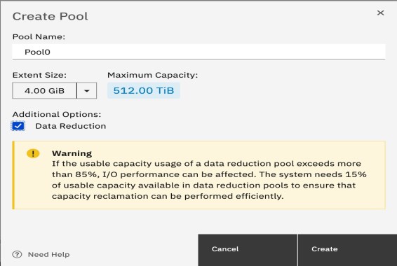
Figure 4-8 Create pool page
2. Create a Data Reduction child pool, as shown in Figure 4-10 on page 148:
a. In the management GUI, select Pools → Pools.
b. Right-click the parent pool you want to create the child pool in, as shown in Figure 4-9 on page 148.

Figure 4-9 Right-click parent pool actions menu
c. Select Create Child Pool.
d. Enter a name for the child pool, as shown in Figure 4-10.
e. Click Create.

Figure 4-10 Create child pool page
3. Add storage to a parent DRP by completing these steps:
a. In the management GUI, select Pools → Pools.
b. Right-click the DRP that you created and select Add Storage.
c. Select from the available storage and allocate capacity to the pool. Click Assign.
4. Create fully-allocated, compressed, deduplicated, or a combination of compressed and deduplicated volumes in the DRP and map them to hosts by completing the following steps:
a. In the management GUI, select Volumes → Volumes.
b. On the Volumes page, click Create Volumes.
c. On the Create Volume page, select the type of volume that you want to create.
d. Enter the following information for the volume:
• Pool
Select a DRP from the list. Compressed, thin-provisioned, and deduplicated volumes, and copies, must be in DRPs.
• Volume details
Enter the quantity, capacity, and name for the volume or volumes that you are creating.
• Capacity savings
Select None (fully-allocated), or Compressed. When compressed is selected, you also can select to use deduplication for the volume that you create.
|
Note: If your system contains self-compressed drives, ensure that the volume is created with Compression enabled. If not, the system cannot calculate accurate available physical capacity.
|

Figure 4-11 Create Volume page
|
Note: Select Create to create the volumes in the DRP without mapping to hosts. If you want to map volumes to hosts later, select Hosts → Hosts → Add Hosts.
|
f. On the Create Mapping page, select Host to display all hosts that are available for mapping. Hosts must support SCSI unmap commands. Verify that the selected host type supports SCSI unmap commands. Click Next.
g. Starting with version 8.3.1 the system will try to map the SCSI LUN ID the same on all Host clusters, if you want to assign specific IDs then select the Self Assign checkbox.

Figure 4-12 The Create Mapping page
Using the command line interface
To create DRPs by using the CLI, complete the following steps:
1. To create a DRP, enter the following command:
mkmdiskgrp -name pool_name -ext extent_size -datareduction yes
Where pool_name is the name of the pool and extent_size is the extent size of the pool. You can create DRPs only as parent pools, not child pools.
2. To create a compressed volume within a DRP, enter the following command:
mkvolume -name name -pool storage_pool_name -size disk_size -compressed
3. Where name is the name of the new volume, storage_pool_name is the name of the DRP, and disk_size is the capacity of the volume.
4. To map the volume to a host, enter the following command:
mkvdiskhostmap -host host_name vdisk_name
Where host_name is the name of the host and vdisk_name is the name of the volume.
For more information, see this IBM Documentation web page.
Monitor the physical capacity of DRPs in the management GUI by selecting Pools → Pools. In the command line interface, use the lsmdiskgrp command to display the physical capacity of a DRP.
4.4.2 Adding external MDisks to existing storage pools
If MDisks are being added to an IBM FlashSystem cluster, it is likely because you want to provide more capacity. In Easy Tier enabled pools, the storage-pool balancing feature guarantees that the newly added MDisks are automatically populated with extents that come from the other MDisks. Therefore, manual intervention is not required to rebalance the capacity across the available MDisks.
|
Important: When adding external MDisks, the system does not know to which tier the MDisk belongs. You must ensure that you specify or change the tier type to match the tier type of the MDisk.
This specification is vital to ensure that Easy Tier keeps a pool as a single tier pool and balances across all MDisks, or Easy Tier adds the MDisk to the correct tier in a multitier pool.
Failure to set the correct tier type creates a performance problem that might be difficult to diagnose in the future.
|
The tier_type can be changed using the CLI:
chmdisk -tier <new_tier> <mdisk>
For more information see 4.6.9, “Easy Tier settings” on page 189.
Adding MDisks to storage pools is a simple task, but it is suggested that you perform some checks in advance especially when adding external MDisks.
Checking access to new MDisks
Be careful when you add external MDisks to existing storage pools to ensure that the availability of the storage pool is not compromised by adding a faulty MDisk. The reason is that loss of access to a single MDisk causes the entire storage pool to go offline.
In IBM Spectrum Virtualize, there is a feature that tests an MDisk automatically for reliable read/write access before it is added to a storage pool. Therefore, user action is not required. The test fails under the following conditions:
•One or more nodes cannot access the MDisk through the chosen controller port.
•I/O to the disk does not complete within a reasonable time.
•The SCSI inquiry data that is provided for the disk is incorrect or incomplete.
•The IBM Spectrum Virtualize cluster suffers a software error during the MDisk test.
Image-mode MDisks are not tested before they are added to a storage pool because an offline image-mode MDisk does not take the storage pool offline. Therefore, the suggestion here is to use a dedicated storage pool for each image mode MDisk. This preferred practice makes it easier to discover what the MDisk is going to be virtualized as, and reduces the chance of human error.
Persistent reserve
A common condition where external MDisks can be configured by IBM FlashSystem, but cannot perform read/write, is when a persistent reserve is left on a LUN from a previously attached host.
In this condition, rezone the back-end storage and map them back to the host that is holding the reserve. Alternatively, map them to another host that can remove the reserve by using a utility such as the Microsoft Windows SDD Persistent Reserve Tool.
4.4.3 Renaming MDisks
After you discover MDisks, rename them from their IBM FlashSystem default name. This can help during problem isolation and avoid confusion that can lead to an administrative error by using a naming convention for MDisks that associates the MDisk with the controller and array.
When multiple tiers of storage are on the same IBM FlashSystem cluster, you might also want to indicate the storage tier in the name. For example, you can use R5 and R10 to differentiate RAID levels, or you can use T1, T2, and so on, to indicate the defined tiers.
|
Preferred practice: For MDisks, use a naming convention that associates the MDisk with its corresponding controller and array within the controller, such as DS8K_<extent pool name/id>_<volume id>.
|
4.4.4 Removing MDisks from storage pools
You might want to remove MDisks from a storage pool (for example, when you decommission a storage controller). When you remove MDisks from a storage pool, consider whether to manually migrate extents from the MDisks. It is also necessary to make sure that you remove the correct MDisks.
|
Sufficient space: The removal of MDisks occurs only if sufficient space is available to migrate the volume data to other extents on other MDisks that remain in the storage pool. After you remove the MDisk from the storage pool, it takes time to change the mode from managed to unmanaged, depending on the size of the MDisk that you are removing.
|
When you remove the MDisk made of internal disk drives from the storage pool on an IBM FlashSystem, the MDisk is deleted. This process also deletes the array on which this MDisk was built, and converts all drives that were included in this array to a candidate state. You can now use those disk drives to create another array of a different size and RAID type, or you can use them as hot spares.
Migrating extents from the MDisk to be deleted
If an MDisk contains volume extents, you must move these extents to the remaining MDisks in the storage pool. Example 4-3 shows how to list the volumes that have extents on an MDisk by using the CLI.
Example 4-3 Listing of volumes that have extents on an MDisk to be deleted
IBM_2145:itsosvccl1:admin>lsmdiskextent mdisk14
id number_of_extents copy_id
5 16 0
3 16 0
6 16 0
8 13 1
9 23 0
8 25 0
|
DRP restriction: The lsmdiskextent command does not provide accurate extent usage for thin-provisioned or compressed volumes on DRPs.
|
Specify the -force flag on the rmmdisk command, or select the corresponding option in the GUI. Both actions cause IBM FlashSystem to automatically move all used extents on the MDisk to the remaining MDisks in the storage pool.
Alternatively, you might want to manually perform the extent migrations. Otherwise, the automatic migration randomly allocates extents to MDisks (and areas of MDisks). After all of the extents are manually migrated, the MDisk removal can proceed without the -force flag.
Verifying the identity of an MDisk before removal
External MDisks must appear to the IBM FlashSystem cluster as unmanaged before their controller LUN mapping is removed. Unmapping LUNs from IBM FlashSystem that are still part of a storage pool results in the storage pool that goes offline and affects all hosts with mappings to volumes in that storage pool.
If the MDisk was named using the preferred practices, the correct LUNs are easier to identify. However, ensure that the identification of LUNs that are being unmapped from the controller match the associated MDisk on IBM FlashSystem by using the Controller LUN Number field and the unique identifier (UID) field.
The UID is unique across all MDisks on all controllers. However, the controller LUN is unique only within a specified controller and for a certain host. Therefore, when you use the controller LUN, check that you are managing the correct storage controller and that you are looking at the mappings for the correct IBM FlashSystem host object.
|
Tip: Renaming your back-end storage controllers as recommended also helps you with MDisk identification.
|
For more information about how to correlate back-end volumes (LUNs) to MDisks, see “Correlating the back-end volume with the MDisk” on page 153.
Correlating the back-end volume with the MDisk
The correct correlation between the back-end volume (LUN) with the external MDisk is crucial to avoid mistakes and possible outages. You can correlate the back-end volume with MDisk for DS8000 series, XIV, and FlashSystem V7000 storage controllers.
DS8000 LUN
The LUN ID only uniquely identifies LUNs within the same storage controller. If multiple storage devices are attached to the same IBM FlashSystem cluster, the LUN ID must be combined with the worldwide node name (WWNN) attribute to uniquely identify LUNs within the IBM FlashSystem cluster.
To get the WWNN of the DS8000 controller, take the first 16 digits of the MDisk UID and change the first digit from 6 to 5, such as 6005076305ffc74c to 5005076305ffc74c. When detected as IBM FlashSystem ctrl_LUN_#, the DS8000 LUN is decoded as 40XX40YY00000000, where XX is the logical subsystem (LSS) and YY is the LUN within the LSS. As detected by the DS8000, the LUN ID is the four digits starting from the 29th digit, as shown in the Example 4-4.
Example 4-4 DS8000 UID example
6005076305ffc74c000000000000100700000000000000000000000000000000
In Example 4-4, you can identify the MDisk supplied by the DS8000, which is LUN ID 1007.
XIV system volumes
Identify the XIV volumes by using the volume serial number and the LUN that is associated with the host mapping. The example in this section uses the following values:
•Serial number: 897
•LUN: 2
Complete the following steps:
1. To identify the volume serial number, right-click a volume and select Properties. Example 4-5 on page 154 shows the Volume Properties dialog box that opens.
2. To identify your LUN, in the volumes by Hosts view, expand your IBM FlashSystem host group and then review the LUN column, as shown in Example 4-5.
3. The MDisk UID field consists of part of the controller WWNN from bits 2 - 13. You might check those bits by using the lscontroller command, as shown in Example 4-5.
Example 4-5 The lscontroller command
IBM_2145:tpcsvc62:admin>lscontroller 10
id 10
controller_name controller10
WWNN 5001738002860000
...
4. The correlation can now be performed by taking the first 16 bits from the MDisk UID field:
– Bits 1 - 13 refer to the controller WWNN, as shown in Example 4-5.
– Bits 14 - 16 are the XIV volume serial number (897) in hexadecimal format (resulting in 381 hex).
– The translation is 0017380002860381000000000000000000000000000000000000000000000000,
where:
• The controller WWNN (bits 2 - 13) is 0017380002860
• The XIV volume serial number that is converted in hex is 381
5. To correlate the IBM FlashSystem ctrl_LUN_#:
a. Convert the XIV volume number in hexadecimal format.
b. Check the last three bits from the IBM FlashSystem ctrl_LUN_#.
In this example, the number is 0000000000000002, as shown in Figure 4-13 on page 155.
FlashSystem volumes
The IBM FlashSystem solution is built upon the IBM Spectrum Virtualize technology base and uses similar terminology.
Complete the following steps to correlate the IBM FlashSystem volumes with the external MDisks that are seen by the virtualizer:
1. From the back-end IBM FlashSystem side, check the Volume UID field for the volume that was presented to the virtualizer, as shown in Figure 4-13 on page 155.

Figure 4-13 FlashSystem volume details
2. On the Host Maps tab, check the SCSI ID number for the specific volume, as shown in Figure 4-14. This value is used to match the virtualizer ctrl_LUN_# (in hexadecimal format).

Figure 4-14 FlashSystem volume details for host maps
3. At the virtualizer, review the MDisk details and compare the MDisk UID field with the FlashSystem Volume UID, as shown in Figure 4-15. The first 32 bits should be the same.

Figure 4-15 IBM SAN Volume Controller MDisk details for IBM FlashSystem volumes
4. Double-check that the virtualizer ctrl_LUN_# is the IBM FlashSystem SCSI ID number in hexadecimal format. In this example, the number is 0000000000000005.
4.4.5 Remapping managed MDisks
Generally, you do not unmap managed external MDisks from IBM FlashSystem because this process causes the storage pool to go offline. However, if managed MDisks were unmapped from IBM FlashSystem for a specific reason, the LUN must present the same attributes to IBM FlashSystem before it is mapped back. Such attributes include UID, subsystem identifier (SSID), and LUN_ID.
If the LUN is mapped back with different attributes, IBM FlashSystem recognizes this MDisk as a new MDisk. In this case, the associated storage pool does not come back online. Consider this situation for storage controllers that support LUN selection because selecting a different LUN ID changes the UID. If the LUN was mapped back with a different LUN ID, it must be mapped again by using the previous LUN ID.
4.4.6 Controlling extent allocation order for volume creation
When creating a new volume on a standard pool, the allocation of extents is performed using a round-robin algorithm, taking one extent from each MDisk in the pool in turn.
The first MDisk to allocate an extent from is chosen in a pseudo-random way rather than always starting from the same MDisk. The pseudo-random algorithm avoids the situation where the “striping effect” inherent in a round-robin algorithm places the first extent for many volumes on the same MDisk.
Placing the first extent of a number of volumes on the same MDisk might lead to poor performance for workloads that place a large I/O load on the first extent of each volume or that create multiple sequential streams.
However, this allocation pattern is unlikely to remain for long because Easy Tier balancing begins to move the extents to balance the load evenly across all MDisk in the tier. The hot and cold extents also are moved between tiers.
In a multi-tier pool, the middle tier is used by default for new volume creation. If free space is not available in the middle tier, the cold tier will be used if it exists. If the cold tier does not exist, the hot tier will be used. For more information on Easy Tier, see 4.6, “Easy Tier, tiered and balanced storage pools” on page 169.
|
DRP restriction: With compressed and deduplicated volumes on DRP, the extent distribution cannot be checked across the MDisks. Initially, only a minimal number of extents are allocated to the volume, based on the rsize parameter.
|
4.5 Considerations when using encryption
IBM SAN Volume Controller (since 2145-DH8) and all IBM FlashSystem support optional encryption of data at rest. This support protects against the potential exposure of sensitive user data and user metadata that is stored on discarded, lost, or stolen storage devices. To use encryption on the system, an encryption license is required for each IBM FlashSystem I/O Group that support encryption.
|
Note: Consider the following points:
•Check if you have the required IBM Security™ Key Lifecycle Manager licenses on hand. Consider redundancy and high-availability regarding Key Lifecycle Manager servers.
•In IBM Spectrum Virtualize code level V8.2.1 and later, Gemalto Safenet KeySecure also is supported. In code level V8.4.1 and later, Thales CipherTrust Manager is supported. For more information about the supported key servers see, this IBM Support web page.
|
4.5.1 General considerations
USB encryption, key server encryption, or both can be enabled on the system. The system supports IBM Security Key Lifecycle Manager version 2.6.0 or later for enabling encryption with a key server. To encrypt data that is stored on drives, the IBM FlashSystem I/O Groups that are capable of encryption must be licensed and configured to use encryption.
When encryption is activated and enabled on the system, valid encryption keys must be present on the system when the system unlocks the drives or the user generates a new key. If USB encryption is enabled on the system, the encryption key must be stored on USB flash drives that contain a copy of the key that was generated when encryption was enabled. If key server encryption is enabled on the system, the key is retrieved from the key server.
It is not possible to convert the existing data to an encrypted copy. You can use the volume migration function to migrate the data to an encrypted storage pool or encrypted child pool. Alternatively, you can also use the volume mirroring function to add a copy to an encrypted storage pool or encrypted child pool and delete the unencrypted copy after the migration.
|
Note: Hot Spare Nodes also need encryption licenses if they are to be used to replace the failed nodes that support encryption.
|
Before you activate and enable encryption, you must determine the method of accessing key information during times when the system requires an encryption key to be present. The system requires an encryption key to be present during the following operations:
•System power-on
•System restart
•User initiated rekey operations
•System recovery
Several factors must be considered when planning for encryption:
•Physical security of the system
•Need and benefit of manually accessing encryption keys when the system requires
•Availability of key data
•Encryption license is purchased, activated, and enabled on the system
•Using Security Key Lifecycle Manager clones
|
Note: It is suggested that you use IBM Security Key Lifecycle Manager version 2.7.0 or later for new clone end points created on the system.
|
For configuration details about IBM FlashSystem encryption, see the following publications:
•Implementing the IBM FlashSystem with IBM Spectrum Virtualize V8.4.2, SG24-8506
•Implementing the IBM SAN Volume Controller with IBM Spectrum Virtualize V8.4.2, SG24-8507
4.5.2 Hardware and software encryption
Encryption can be performed in IBM FlashSystem devices by using one of two methods: hardware encryption and software encryption.
Both methods protect against the potential exposure of sensitive user data that are stored on discarded, lost, or stolen media. Both methods also can facilitate the warranty return or disposal of hardware. The method to be used for encryption is chosen automatically by the system based on the placement of the data.
Figure 4-16 shows encryption placement in the lower layers of the IBM FlashSystem software stack.

Figure 4-16 Encryption placement in lower layers of the IBM FlashSystem software stack
Hardware encryption only storage pool
Hardware encryption features the following characteristics:
•Algorithm is built in SAS chip for all SAS attached drives, or built into the drive itself for NVMe attached drives (FCM, IS NVMe and SCM).
•No system overhead.
•Only available to direct attached SAS disks.
•Can only be enabled when you create internal arrays.
•Child pools cannot be encrypted if the parent storage pool is not encrypted.
•Child pools are automatically encrypted if the parent storage pool is encrypted, but can have different encryption keys.
•DRP child pools can only use the same encryption key as their parent.
Software encryption only storage pool
Software encryption features the following characteristics:
•The algorithm is running at the interface device driver.
•Uses special CPU instruction set and engines (AES_NI).
•Allows encryption for virtualized external storage controllers, which are not capable of self-encryption.
•Less than 1% system overhead.
•Only available to virtualized external storage.
•Can only be enabled when you create storage pools and child pools made up of virtualized external storage.
•Child pools can be encrypted even if the parent storage pool is not encrypted.
Mixed encryption in a storage pool
It is possible to mix hardware and software encryption in a storage pool, as shown in Figure 4-17.

Figure 4-17 Mixed encryption in a storage pool
However, if you want to create encrypted child pools from an unencrypted storage pool containing a mix of internal arrays and external MDisks. the following restrictions apply:
•The parent pool must not contain any unencrypted internal arrays.
•All IBM FlashSystem nodes in the system must support software encryption and have an activated encryption license.
|
Note: An encrypted child pool created from an unencrypted parent storage pool reports as unencrypted if the parent pool contains unencrypted internal arrays. Remove these arrays to ensure that the child pool is fully encrypted.
|
The general rule is to not mix different types of MDisks in a storage pool, unless it is intended to use the Easy Tier tiering function. In this scenario, the internal arrays must be encrypted if you want to create encrypted child pools from an unencrypted parent storage pool. All methods of encryption use the same encryption algorithm, the same key management infrastructure, and the same license.
|
Note: Always implement encryption on the self-encryption capable back-end storage, such as IBM FlashSystem, IBM Storwize, IBM XIV, IBM FlashSystem A9000, and IBM DS8000, to avoid potential system overhead.
|
Declare or identify the self-encrypted virtualized external MDisks as encrypted on IBM FlashSystem by setting the -encrypt option to yes in the chmdisk command, as shown in Example 4-6. This configuration is important to avoid IBM FlashSystem trying to encrypt them again.
Example 4-6 Command to declare or identify a self-encrypted MDisk from a virtualized external storage
IBM_2145:ITSO_DH8_A:superuser>chmdisk -encrypt yes mdisk0
|
Note: It is important to declare or identify the self-encrypted MDisks from a virtualized external storage before creating an encrypted storage pool or child pool on IBM FlashSystem.
|
4.5.3 Encryption at rest with USB keys
The following section describes the characteristics of using USB flash drives for encryption and the available options to access the key information.
USB flash drives have the following characteristics:
•Physical access to the system is required to process a rekeying operation
•No mechanical components to maintain with almost no read operations or write operations to the USB flash drive.
•Inexpensive to maintain and use.
•Convenient and easy to have multiple identical USB flash drives available as backups.
Two options are available for accessing key information on USB flash drives:
•USB flash drives are left inserted in the system at all times.
If you want the system to restart automatically, a USB flash drive must be left inserted in all the nodes on the system. When you power on, all nodes then have access to the encryption key. This method requires that the physical environment where the system is located is secure. If the location is secure, it prevents an unauthorized person from making copies of the encryption keys, stealing the system, or accessing data that is stored on the system.
•USB flash drives are not left inserted into the system except as required
For the most secure operation, do not keep the USB flash drives inserted into the nodes on the system. However, this method requires that you manually insert the USB flash drives that contain copies of the encryption key in the nodes during operations that the system requires an encryption key to be present. USB flash drives that contain the keys must be stored securely to prevent theft or loss.
4.5.4 Encryption at rest with key servers
The following section describes the characteristics of using key servers for encryption and essential recommendations for key server configuration with IBM FlashSystem.
Key servers
Key servers have the following characteristics:
•Physical access to the system is not required to process a rekeying operation.
•Support for businesses that have security requirements not to use USB ports.
•Strong key generation.
•Key self-replication and automatic backups.
•Implementations follow an open standard that aids in interoperability.
•Audit detail.
•Ability to administer access to data separately from storage devices.
Encryption key servers create and manage encryption keys that are used by the system. In environments with a large number of systems, key servers distribute keys remotely without requiring physical access to the systems. A key server is a centralized system that generates, stores, and sends encryption keys to the system. If the key server provider supports replication of keys among multiple key servers, you can specify up to 4 key servers (one master and three clones) that connect to the system over both a public network or a separate private network.
The system supports using an IBM Security Key Lifecycle Manager key server to enable encryption. All key servers must be configured on the IBM Security Key Lifecycle Manager before defining the key servers in the management GUI. IBM Security Key Lifecycle Manager supports Key Management Interoperability Protocol (KMIP), which is a standard for encryption of stored data and management of cryptographic keys.
IBM Security Key Lifecycle Manager can be used to create managed keys for the system and provide access to these keys through a certificate. If you are configuring multiple key servers, use IBM Security Key Lifecycle Manager 2.6.0.2 or later. The additional key servers (clones) support more paths when delivering keys to the system; however, during rekeying only the path to the primary key server is used. When the system is rekeyed, secondary key servers are unavailable until the primary has replicated the new keys to these secondary key servers.
Replication must complete before keys can be used on the system. You can either schedule automatic replication or complete it manually with IBM Security Key Lifecycle Manager. During replication, key servers are not available to distribute keys or accept new keys. The time a replication completes on the IBM Security Key Lifecycle Manager depends on the number of key servers that are configured as clones, and the amount of key and certificate information that is being replicated.
The IBM Security Key Lifecycle Manager issues a completion message when the replication completes. Verify that all key servers contain replicated key and certificate information before keys are used on the system.
Recommendations for key server configuration
The following section provides some essential recommendations for key server configuration with IBM FlashSystem.
Transport Layer Security
Define the IBM Security Key Lifecycle Manager to use Transport Layer Security version 2 (TLSv2).
The default setting on IBM Security Key Lifecycle Manager since version 3.0.1 is TLSv1.2, but the IBM FlashSystem only supports version 2. On the IBM Security Key Lifecycle Manager, set the value to SSL_TLSv2, which is a set of protocols that includes TLSv1.2.
For more information about the protocols, see this IBM Documentation web page.
Example 4-7 shows the example of a SKLMConfig.properties configuration file. The default path on a Linux based server is /opt/IBM/WebSphere/AppServer/products/sklm/config/SKLMConfig.properties.
Example 4-7 Example of a SKLMConfig.properties configuration file
#Mon Nov 20 18:37:01 EST 2017
KMIPListener.ssl.port=5696
Audit.isSyslog=false
Audit.syslog.server.host=
TransportListener.ssl.timeout=10
Audit.handler.file.size=10000
user.gui.init.config=true
config.keystore.name=defaultKeyStore
tklm.encryption.password=D1181E14054B1E1526491F152A4A1F3B16491E3B160520151206
Audit.event.types=runtime,authorization,authentication,authorization_terminate,resource_management,key_management
tklm.lockout.enable=true
enableKeyRelease=false
TransportListener.tcp.port=3801
Audit.handler.file.name=logs/audit/sklm_audit.log
config.keystore.batchUpdateTimer=60000
Audit.eventQueue.max=0
enableClientCertPush=true
debug=none
tklm.encryption.keysize=256
TransportListener.tcp.timeout=10
backup.keycert.before.serving=false
TransportListener.ssl.protocols=SSL_TLSv2
Audit.syslog.isSSL=false
cert.valiDATE=false
config.keystore.batchUpdateSize=10000
useSKIDefaultLabels=false
maximum.keycert.expiration.period.in.years=50
config.keystore.ssl.certalias=sklm
TransportListener.ssl.port=441
Transport.ssl.vulnerableciphers.patterns=_RC4_,RSA_EXPORT,_DES_
Audit.syslog.server.port=
tklm.lockout.attempts=3
fips=off
Audit.event.outcome=failure
Self-signed certificate type and validity period
The default certificate type on IBM Security Key Lifecycle Manager server and IBM FlashSystem is RSA. If you use different certificate type, make sure you match the certificate type on both end. The default certificate validity period is 1095 days on IBM Security Key Lifecycle Manager server and 5475 days on IBM FlashSystem.
You can adjust the validity period to comply with specific security policies and always match the certificate validity period on IBM FlashSystem and IBM Security Key Lifecycle Manager server. A mismatch will cause certificate authorization error and lead to unnecessary certificate exchange.
Figure 4-18 shows the default certificate type and validity period on IBM FlashSystem.

Figure 4-18 Update certificate on IBM FlashSystem
Figure 4-19 shows the default certificate type and validity period on IBM Security Key Lifecycle Manager server.

Figure 4-19 Create self-signed certificate on IBM Security Key Lifecycle Manager server
Device group configuration
The SPECTRUM_VIRT device group is not predefined on IBM Security Key Lifecycle Manager, it must be created based on a GPFS device family as shown in Figure 4-20.

Figure 4-20 Create device group for IBM FlashSystem
By default, IBM FlashSystem the SPECTRUM_VIRT group name is predefined in the encryption configuration wizard. SPECTRUM_VIRT contains all the keys for the managed IBM FlashSystem. However, It is possible to use different device groups as long as they are GPFS device family based. For example, one device group for each environment (Production or Disaster Recovery (DR)). Each device group maintains its own key database, and this approach allows more granular key management.
Clone servers configuration management
The minimum replication interval on IBM Security Key Lifecycle Manager is one hour, as shown in Figure 4-21. It is more practical to perform backup and restore or manual replication for the initial configuration to speed up the configuration synchronization.
Also, the rekey process creates a new configuration on the IBM Security Key Lifecycle Manager server, and it is important not to wait for the next replication window but to manually synchronize the configuration to the additional key servers (clones). Otherwise, an error message is generated by the IBM FlashSystem system, which indicates that the key is missing on the clones.
Figure 4-21 shows the replication interval.
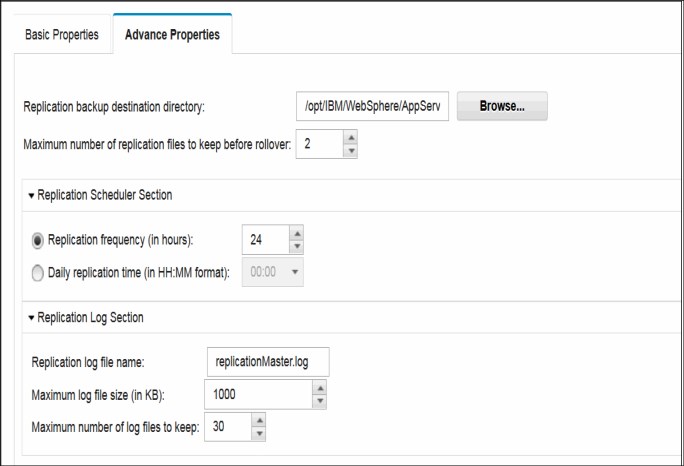
Figure 4-21 SKLM Replication Schedule
Example 4-8 shows an example of manually triggered replication.
Example 4-8 Manually triggered replication
/opt/IBM/WebSphere/AppServer/bin/wsadmin.sh -username SKLMAdmin -password <password> -lang jython -c "print AdminTask.tklmReplicationNow()"
Encryption key management
There is always only one active key for each encryption enabled IBM FlashSystem system. The previously-used key is deactivated after the rekey process. It is possible to delete the deactivated keys to keep the key database tidy and up-to-date.
Figure 4-22 on page 167 shows the keys associated with a device group. In this example, the SG247933_REDBOOK device group contains one encryption-enabled IBM FlashSystem, and it has three associated keys. Only one of the keys is activated, and the other two were deactivated after the rekey process.

Figure 4-22 Keys associated to a device group
Example 4-9 shows an example to check the state of the keys.
Example 4-9 Verify key state
/opt/IBM/WebSphere/AppServer/bin/wsadmin.sh -username SKLMAdmin -password <password> -lang jython
wsadmin>print AdminTask.tklmKeyList('[-uuid KEY-8a89d57-15bf8f41-cea6-4df3-8f4e-be0c36318615]')
CTGKM0001I Command succeeded.
uuid = KEY-8a89d57-15bf8f41-cea6-4df3-8f4e-be0c36318615
alias = mmm008a89d57000000870
key algorithm = AES
key store name = defaultKeyStore
key state = ACTIVE
creation date = 18/11/2017, 01:43:27 Greenwich Mean Time
expiration date = null
wsadmin>print AdminTask.tklmKeyList('[-uuid KEY-8a89d57-74edaef9-b6d9-4766-9b39-7e21d9911011]')
CTGKM0001I Command succeeded.
uuid = KEY-8a89d57-74edaef9-b6d9-4766-9b39-7e21d9911011
alias = mmm008a89d5700000086e
key algorithm = AES
key store name = defaultKeyStore
key state = DEACTIVATED
creation date = 17/11/2017, 20:07:19 Greenwich Mean Time
expiration date = 17/11/2017, 23:18:37 Greenwich Mean Time
wsadmin>print AdminTask.tklmKeyList('[-uuid KEY-8a89d57-ebe5d5a1-8987-4aff-ab58-5f808a078269]')
CTGKM0001I Command succeeded.
uuid = KEY-8a89d57-ebe5d5a1-8987-4aff-ab58-5f808a078269
alias = mmm008a89d5700000086f
key algorithm = AES
key store name = defaultKeyStore
key state = DEACTIVATED
creation date = 17/11/2017, 23:18:34 Greenwich Mean Time
expiration date = 18/11/2017, 01:43:32 Greenwich Mean Time
|
Note: The initial configuration, such as certificate exchange and Transport Layer Security configuration, is only required on the master IBM Security Key Lifecycle Manager server. The restore or replication process duplicates all of the required configurations to the clone servers.
|
If encryption was enabled on a pre-V7.8.0 code level system and the system is updated to V7.8.x or above, you must run a USB rekey operation to enable key server encryption. Run the chencryption command before you enable key server encryption. To perform a rekey operation, run the commands that are shown in Example 4-10.
Example 4-10 Commands to enable key server encryption option on a system upgraded from pre-7.8.0
chencyrption -usb newkey -key prepare
chencryption -usb newkey -key commit
For more information about Encryption with Key Server, see this IBM Documentation web page.
4.6 Easy Tier, tiered and balanced storage pools
Easy Tier was originally developed to provide the maximum performance benefit from a few SSDs or flash drives. Because of their low response times, high throughput, and IOPS-energy-efficient characteristics, SSDs and flash arrays were a welcome addition to the storage system, but initially their acquisition cost per Gigabyte (GB) was more than for HDDs.
By implementing an evolving almost AI-like algorithm, Easy Tier moved the most frequently accessed blocks of data to the lowest latency device. Therefore, it provides an exponential improvement in performance when compared to a small investment in SSD and flash capacity.
The industry moved on in the more than 10 years since Easy Tier was first introduced. The cost of SSD and flash-based technology meant that more users can deploy all-flash environments.
HDD-based large capacity NL-SAS drives are still the most cost-effective online storage devices. Although SSD and flash ended the 15 K RPM and 10 K RPM drive market, it has yet to reach a price point that competes with NL-SAS for lower performing workloads. The use cases for Easy Tier changed, and most deployments now use “flash and trash” approaches, with 50% or more flash capacity and the remainder using NL-SAS.
Easy Tier also provides balancing within a tier. This configuration ensures that no one single component within a tier of the same capabilities is more heavily loaded than another. It does so to maintain an even latency across the tier and help to provide consistent and predictable performance.
As the industry strives to develop technologies that can enable higher throughput and lower latency than even flash, Easy Tier continues to provide user benefits. For example, Storage Class Memory (SCM) technologies, which were introduced to FlashSystem in 2020, now provide lower latency than even flash, but as with flash when first introduced, at a considerably higher cost of acquisition per GB.
Choosing the correct mix of drives and the data placement is critical to achieve optimal performance at the lowest cost. Maximum value can be derived by placing “hot” data with high I/O density and low response time requirements on the highest tier, while targeting lower tiers for “cooler” data, which is accessed more sequentially and at lower rates.
Easy Tier dynamically automates the ongoing placement of data among different storage tiers. It also can be enabled for internal and external storage to achieve optimal performance.
Also, the Easy Tier feature that is called storage pool balancing automatically moves extents within the same storage tier from overloaded to less loaded MDisks. Storage pool balancing ensures that your data is optimally placed among all disks within storage pools.
Storage pool balancing is designed to balance extents between tiers in the same pool to improve overall system performance and to avoid overloading a single MDisk in the pool.
However, considers only performance, it does not consider capacity. Therefore, if two FCM arrays are in a pool and one of them is nearly out of space and the other is empty, Easy Tier does not attempt to move extents between the arrays.
For this reason, it is recommended that if you must increase the capacity on an MDisk, increase the size of the array rather than add an FCM array.
4.6.1 Easy Tier concepts
IBM FlashSystem products implement Easy Tier enterprise storage functions, which were originally designed in conjunction with the development of Easy Tier on IBM DS8000 enterprise class storage systems. It enables automated subvolume data placement throughout different or within the same storage tiers. This feature intelligently aligns the system with current workload requirements and optimizes the usage of high-performance storage, such as SSD, flash and SCM.
Easy Tier reduces the I/O latency for hot spots, but it does not replace storage cache. Both Easy Tier and storage cache solve a similar access latency workload problem. However, these two methods weigh differently in the algorithmic construction that is based on locality of reference, recency, and frequency. Because Easy Tier monitors I/O performance from the device end (after cache), it can pick up the performance issues that cache cannot solve, and complement the overall storage system performance.
The primary benefit of Easy Tier is to reduce latency for hot spots; however, this feature also includes an added benefit where the remaining “medium” (that is, not cold) data has less contention for its resources and performs better as a result (that is, lower latency).
In addition, Easy Tier can be used in a single tier pool to balance the workload across storage MDisks. Is also ensures an even load on all MDisks in a tier or pool. Therefore, bottlenecks and convoying effects are removed when striped volumes are used. In a multitier pool, each tier is balanced.
In general, the storage environment’s I/O is monitored at a volume level, and the entire volume is always placed inside one suitable storage tier. Determining the amount of I/O, moving part of the underlying volume to an appropriate storage tier, and reacting to workload changes is too complex for manual operation. It is in this situation that the Easy Tier feature can be used.
Easy Tier is a performance optimization function that automatically migrates extents that belong to a volume between different storage tiers (see Figure 4-23 on page 171) or the same storage tier (see Figure 4-25 on page 178). Because this migration works at the extent level, it is often referred to as sublogical unit number (LUN) migration. Movement of the extents is dynamic, nondisruptive, and is not visible from the host perspective. As a result of extent movement, the volume no longer has all its data in one tier; rather, it is in two or three tiers, or is balanced between MDisks in the same tier.

Figure 4-23 Easy Tier single volume, multiple tiers
You can enable Easy Tier on a per volume basis, except for non-fully allocated volumes in a DRP where Easy Tier is always enabled. It monitors the I/O activity and latency of the extents on all Easy Tier enabled volumes.
Based on the performance characteristics, Easy Tier creates an extent migration plan and dynamically moves (promotes) high activity or hot extents to a higher disk tier within the same storage pool. Generally, a new migration plan is generated on a stable system once every 24 hours. Instances might occur when Easy Tier reacts within 5 minutes; for example, when detecting an overload situation.
It also moves (demotes) extents whose activity dropped off, or cooled, from higher disk tier MDisks back to a lower tier MDisk. When Easy Tier runs in a storage pool rebalance mode, it moves extents from busy MDisks to less busy MDisks of the same type.
|
Note: Image mode and sequential volumes are not candidates for Easy Tier automatic data placement since all extents for those types of volumes must be on one specific MDisk, and cannot be moved.
|
4.6.2 Easy Tier definitions
Easy Tier measures and classifies each extent into one of its three tiers. It performs this classification process by looking for extents that are the outliers in any system:
1. It looks for the hottest extents in the pool. These extents contain the most frequently accessed data of a suitable workload type (less than 64 KiB I/O). Easy Tier plans to migrate these extents into whatever set of extents that come from MDisks that are designated as the hot tier.
2. It looks for coldest extents in the pool, which are classed as having done < 1 I/O in the measurement period. These extents are planned to be migrated onto extents that come from the MDisks that are designated as the cold tier.It is not necessary for Easy Tier to look for extents to place in the middle tier. By definition, if something is not designated as “hot” or “cold”, it stays or is moved to extents that come from MDisks in the middle tier.
With these three tier classifications, an Easy Tier pool can be optimized.
Internal processing
The Easy Tier function includes the following four main processes:
•I/O Monitoring
This process operates continuously and monitors volumes for host I/O activity. It collects performance statistics for each extent, and derives averages for a rolling 24-hour period of I/O activity.
Easy Tier makes allowances for large block I/Os; therefore, it considers only I/Os of up to 64 kilobytes (KiB) as migration candidates.
This process is efficient and adds negligible processing resource to the IBM FlashSystem nodes.
•Data Placement Advisor (DPA)
The DPA uses workload statistics to make a cost-benefit decision as to which extents are to be candidates for migration to a higher performance tier.
This process also identifies extents that can be migrated back to a lower tier.
•Data Migration Planner (DMP)
By using the extents that were previously identified, the DMP builds the extent migration plans for the storage pool. The DMP builds two plans:
– The Automatic Data Relocation (ADR mode) plan to migrate extents across adjacent tiers.
– The Rebalance (RB mode) plan to migrate extents within the same tier.
•Data migrator
This process involves the actual movement or migration of the volume’s extents up to, or down from, the higher disk tier. The extent migration rate is capped so that a maximum of up to 12 GiB every five minutes is migrated, which equates to approximately 3.4TiB per day that is migrated between disk tiers.
|
Note: You can increase the target migration rate to 48 GiB every five minutes by temporarily enabling accelerated mode. See “Easy Tier acceleration” on page 190.
|
When active, Easy Tier performs the following actions across the tiers:
•Promote
Moves the hotter extents to a higher performance tier with available capacity. Promote occurs within adjacent tiers.
•Demote
Demotes colder extents from a higher tier to a lower tier. Demote occurs within adjacent tiers.
•Swap
Exchanges cold extent in an upper tier with hot extent in a lower tier.
•Warm demote
Prevents performance overload of a tier by demoting a warm extent to a lower tier. This process is triggered when bandwidth or IOPS exceeds predefined threshold. If you see these operations, it is a trigger to suggest you should add additional capacity to the higher tier.
•Warm promote
This feature addresses the situation where a lower tier suddenly becomes very active. Instead of waiting for the next migration plan, Easy Tier can react immediately. Warm promote acts in a similar way to warm demote. If the 5-minute average performance shows that a layer is overloaded, Easy Tier immediately starts to promote extents until the condition is relieved. This is often referred to as “overload protection”.
•Cold demote
Demotes inactive (or cold) extents that are on a higher performance tier to its adjacent lower-cost tier. In that way Easy Tier automatically frees extents on the higher storage tier before the extents on the lower tier become hot. Only supported between HDD tiers.
•Expanded cold demote
Demotes appropriate sequential workloads to the lowest tier to better use nearline disk bandwidth.
•Auto rebalance
Redistributes extents within a tier to balance usage across MDisks for maximum performance. This process moves hot extents from high used MDisks to low used MDisks, and exchanges extents between high-use MDisks and low-use MDisks.
•Space reservation demote
Introduced in code version 8.4.0, to prevent out-of-space conditions, EasyTier stops the migration of new data into a tier, and if necessary, migrates extents to a lower tier.
Easy Tier attempts to migrate the most active volume extents up to SSD first.
If a new migration plan is generated before the completion of the previous plan, the previous migration plan and queued extents that are not yet relocated are abandoned. However, migrations that are still applicable are included in the new plan.
|
Note: Extent migration occurs only between adjacent tiers. For instance, in a three-tiered storage pool, Easy Tier will not move extents from the flash tier directly to the nearline tier and vice versa without moving them first to the enterprise tier.
|
Easy Tier extent migration types are shown in Figure 4-24.

Figure 4-24 Easy Tier extent migration types
4.6.3 Easy Tier operating modes
Easy Tier includes the following main operating modes:
•Off
•On
•Automatic
•Measure
Easy Tier is a licensed feature on some FlashSystem 50x0 systems. If the license is not present and Easy Tier is set to Auto or On, the system runs in Measure mode.
|
Options: The Easy Tier function can be turned on or off at the storage pool level and at the volume level, except for non fully-allocated volumes in a DRP where Easy Tier is always enabled.
|
Easy Tier off mode
With Easy Tier turned off, statistics are not recorded, and cross-tier extent-migration does not occur.
Measure mode
Easy Tier can be run in an evaluation or measurement-only mode and collects usage statistics for each extent in a storage pool where the Easy Tier value is set to measure.
This collection is typically done for a single-tier pool, so that the benefits of adding additional performance tiers to the pool can be evaluated before any major hardware acquisition.
The heat and activity of each extent can be viewed in the GUI by clicking Monitoring → Easy Tier Reports. For more information, see 4.6.10, “Monitoring Easy Tier using the GUI” on page 191.
Automatic mode
In Automatic mode, the storage pool parameter -easytier auto must be set, and the volumes in the pool must have -easytier set to on.
The behavior of Easy Tier depends on the pool configuration. Consider the following points:
•If the pool only contains MDisks with a single tier type, the pool is in balancing mode.
•If the pool contains MDisks with more than one tier type, the pool runs automatic data placement and migration in addition to balancing within each tier.
Dynamic data movement is transparent to the host server and application users of the data, other than providing improved performance. Extents are automatically migrated, as explained in “Implementation rules” on page 184.
There might be situations where the Easy Tier setting is “auto” however the system is running in monitoring mode only. For example, with unsupported tier types or if you have not enabled the Easy Tier license. See Table 4-8 on page 180
The GUI provides the same reports as available in measuring mode and, in addition, provide the data movement report that shows the breakdown of the actual migration events triggered by Easy Tier. These migrations are reported in terms of the migration types, as described in “Internal processing” on page 172.
Easy Tier on mode
This mode forces Easy Tier to perform the tasks as in Automatic mode.
For example, when Easy Tier detects an unsupported set of tier types in a pool, as outlined in Table 4-8 on page 180, using On mode will force Easy Tier to the active state and it will perform to the best of its ability. The system raises an alert and there is an associated Directed Maintenance Procedure that guides you to fix the unsupported tier types.
|
Important: Avoid creating a pool with more than three tiers. Although the system attempts to create generic hot, medium, and cold “buckets”, you might end up with Easy Tier that is running in measure mode only.
These configurations are unsupported because they can cause a performance problem in the longer term; for example, disparate performance within a single tier.
The ability to override the automatic mode is provided to enable temporary migration from an older set of tiers to new tiers and must be rectified as soon as possible.
|
Storage pool balancing
This feature assesses the extents that are written in a pool, and balances them automatically across all MDisks within the pool. This process works with Easy Tier when multiple classes of disks exist in a single pool. In this case, Easy Tier moves extents between the different tiers, and storage pool balancing moves extents within the same tier, to enable a balance in terms of workload across all MDisks that belong to a given tier.
Balancing is when you maintain equivalent latency across all MDisks in a given tier, this can result in different capacity usage across the MDisks. However, performance balancing is preferred over capacity-balancing in most cases.
The process automatically balances existing data when new MDisks are added into an existing pool, even if the pool only contains a single type of drive.
Balancing is automatically active on all storage pools, no matter the Easy Tier setting. For a single tier pool the Easy Tier state will report as balancing.
|
Note: Storage pool balancing can be used to balance extents when mixing different size disks of the same performance tier. For example, when adding larger capacity drives to a pool with smaller capacity drives of the same class, storage pool balancing redistributes the extents to take advantage of the additional performance of the new MDisks.
|
Easy Tier mode settings
The Easy Tier setting can be changed on a storage pool and volume level. Depending on the Easy Tier setting and the number of tiers in the storage pool, Easy Tier services might function in a different way. Table 4-6 lists possible combinations of Easy Tier setting.
Table 4-6 Easy Tier settings
|
Storage pool Easy Tier setting
|
Number of tiers in the storage pool
|
Volume copy Easy Tier setting
|
Volume copy Easy Tier status
|
|
Off
|
One or more
|
off
|
inactive (see note 2)
|
|
on
|
inactive (see note 2)
| ||
|
Measure
|
One or More
|
off
|
measured (see note 3)
|
|
on
|
measured (see note 3)
| ||
|
Auto
|
One
|
off
|
measured (see note 3)
|
|
on
|
balanced (see note 4)
| ||
|
Two - four
|
off
|
measured (see note 3)
| |
|
on
|
active (see note 5 & 6)
| ||
|
Five
|
any
|
measured (see note 3)
| |
|
On
|
One
|
off
|
measured (see note 3)
|
|
on
|
balanced (see note 4)
| ||
|
Two - four
|
off
|
measured (see note 3)
| |
|
on
|
active (see note 5)
| ||
|
Five
|
off
|
measured (see note 3)
| |
|
on
|
active (see note 6)
|
|
1. If the volume copy is in image or sequential mode, or is being migrated, the volume copy Easy Tier status is measured rather than active.
2. When the volume copy status is inactive, no Easy Tier functions are enabled for that volume copy.
3. When the volume copy status is measured, the Easy Tier function collects usage statistics for the volume, but automatic data placement is not active.
4. When the volume copy status is balanced, the Easy Tier function enables performance-based pool balancing for that volume copy.
5. When the volume copy status is active, the Easy Tier function operates in automatic data placement mode for that volume.
6. When five tiers (or some four-tier) configurations are used and Easy Tier is in the On state, Easy Tier is forced to operate but might not behave exactly as expected. See Table 4-8 on page 180
The default Easy Tier setting for a storage pool is Auto, and the default Easy Tier setting for a volume copy is On. Therefore, Easy Tier functions, except pool performance balancing, are disabled for storage pools with a single tier. Automatic data placement mode is enabled by default for all striped volume copies in a storage pool with two or more tiers.
|
4.6.4 MDisk tier types
The three Easy Tier tier types (“hot”, “medium”, and “cold”) are generic “buckets” that Easy Tier uses to build a set of extents that belong to each tier. You must tell Easy Tier which MDisks belong to which bucket.
The type of disk and RAID geometry used by internal or external MDisks defines their expected performance characteristics. These characteristics are used to help define a tier type for each MDisk in the system.
Five tier types can be assigned. The tables in this section use the numbers from this list as a shorthand for the tier name:
1. tier_scm that represents Storage Class Memory MDisks
2. tier0_flash that represents enterprise flash technology, including FCM
3. tier1_flash that represents lower performing tier1 flash technology (lower DWPD)
4. tier_enterprise that represents enterprise HDD technology (both 10 K and 15 K RPM)
5. tier_nearline that represents nearline HDD technology (7.2 K RPM)
Consider the following points:.
•Easy Tier is designed to operate with up to 3 tiers of storage, “hot”, “medium”, “cold”
•An MDisk can only belong to one tier type.
•Today, five MDisk tier-types exist.
•Internal MDisks have their tier type set automatically.
•External MDisks default to the “enterprise” tier and might need to be changed by the user.
•The number of MDisk tier-types found in a pool will determine if the pool is a single-tier pool or a multi-tier pool.
|
Attention: As described in 4.6.5, “Changing the tier type of an MDisk” on page 181, IBM FlashSystem do not automatically detect the type of external MDisks. Instead, all external MDisks are initially put into the enterprise tier by default. The administrator must then manually change the MDisks tier and add them to storage pools.
|
Single-tier storage pools
Figure 4-25 shows a scenario in which a single storage pool is populated with MDisks that are presented by an external storage controller. In this solution, the striped volumes can be measured by Easy Tier, and can benefit from storage pool balancing mode, which moves extents between MDisks of the same type.

Figure 4-25 Single tier storage pool with striped volume
MDisks that are used in a single-tier storage pool should have the same hardware characteristics. These characteristics include the same RAID type, RAID array size, disk type, disk RPM, and controller performance characteristics.
For external MDisks, attempt to create all MDisks with the same RAID geometry (number of disks). If this is not possible, you can modify the Easy Tier load setting to manually balance the workload; however, care must be taken. For more information, see “MDisk Easy Tier load” on page 190.
For internal MDisks, the system can cope with different geometries as the number of drives will be reported to Easy Tier, which then uses the Overload Protection information to balance the workload appropriately. See 4.6.6, “Easy Tier overload protection” on page 183.
Multi-tier storage pools
A multi-tier storage pool has a mix of MDisks with more than one type of MDisk tier attribute. This pool can be, for example, a storage pool that contains a mix of enterprise and SSD MDisks or enterprise and NL-SAS MDisks.
Figure 4-26 shows a scenario in which a storage pool is populated with three different MDisk types:
•One belonging to an SSD array
•One belonging to an SAS HDD array
•One belonging to an NL-SAS HDD array)
Although Figure 4-26 shows RAID 5 arrays, other RAID types also can be used.

Figure 4-26 Multitier storage pool with striped volume
|
Note: If you add MDisks to a pool and they have (or you assign) more than three tier types, Easy Tier will try to group two or more of the tier types together into a single “bucket” and use them both as either the “middle” or “cold” tier. The groupings are described in table Table 4-8 on page 180
However, overload protection and pool balancing might result in a bias on the load being placed on those MDisks despite them being in the same “bucket”
|
Easy Tier mapping to MDisk tier types
The five MDisk tier-types are mapped to the three Easy Tier tiers depending on the pool configuration, as shown in Table 4-7.
Table 4-7 Recommended 3-tier Easy Tier mapping policy
|
Tier mix
|
1+2,
1+3,
1+4,
1+5
|
2+3,
2+4,
2+5
|
3+4,
3+5
|
4+5
|
1+2+3,
1+2+4,
1+2+5
|
1+3+4,
1+3+5
|
1+4+5,
2+4+5,
3+4+5
|
2+3+4,
2+3+5
|
|
Hot Tier
|
1
|
2
|
|
|
1
|
1
|
1 or
2 or
3
|
2
|
|
Middle Tier
|
2 or
3 or
4 or
|
3 or
4 or
|
3
|
4
|
2
|
3
|
4
|
3
|
|
Cold Tier
|
5
|
5
|
4 or 5
|
5
|
3 or
4 or
5
|
4 or
5
|
5
|
4 or
5
|
Four- and Five-Tier pools
In general, Easy Tier will try to place tier_enterprise (4)- and tier1_flash (3)-based tiers into the one bucket to reduce the number of tiers defined in a pool to 3. See Table 4-8.
Table 4-8 4 and 5 Tier mapping policy4 and 5 Tier mapping policy
|
Tier Mix
|
1+2+3+4,
1+2+3+5,
1+2+4+5
|
1+3+4+5,
2+3+4+5
|
1+2+3+4+5
|
|
Hot Tier
|
Not supported: measure only
|
1 or 2
|
Not supported: measure only
|
|
Middle Tier
|
3 & 4
| ||
|
Cold Tier
|
5
|
If you create a pool with all five tiers or one of the unsupported four-tier pools and Easy Tier is set to “auto” mode, Easy Tier enters “measure” mode and measures the statistics but does not move any extents. To return to a supported tier configuration, remove one or more MDisks.
|
Important: Avoid creating a pool with more than three tiers. Although the system attempts to create “buckets”, the result might be that Easy Tier runs in measure mode only.
|
Temporary unsupported 4 or 5 tier mapping
If you need to temporarily define four or five in a pool, and you end up with one of the unsupported configurations, you can force Easy Tier to migrate data by setting the Easy Tier mode to “on”.
|
Attention: Extreme caution should be deployed and a full understanding of the implications should be made before forcing Easy Tier to run in this mode.
|
This setting is provided to allow temporary migrations where it is unavoidable to create one of these unsupported configurations. The implications are that long-term use in this mode can cause performance issues due to the grouping of unlike MDisks within a single Easy Tier tier.
For these configurations, the following mapping in Table 4-9 will be used by Easy Tier.
Table 4-9 Unsupported temporary 4 and 5 Tier mapping policy
|
Tier mix
|
1+2+3+4,
1+2+3+5
|
1+2+4+5
|
1+2+3+4+5
|
|
Hot Tier
|
1
|
1
|
1
|
|
Middle Tier
|
2 & 3
|
2
|
2 & 3
|
|
Cold Tier
|
4 or 5
|
4 & 5
|
4 & 5
|
|
comment
|
See Note 1
|
See Note 2
|
See Note 1 & 2
|
|
Note: The following notes apply to Table 4-9:
•Note 1: In these configurations, Enterprise HDD and Nearline HDD are placed into the cold tier. These two drive types feature different latency characteristics and the difference can skew the metrics that are measured by Easy Tier for the cold tier.
•Note 2: In these configurations, Tier0 and Tier 1 flash devices are placed in the middle tier. The different drive writes per day does not make the most efficient use of the Tier0 flash.
|
4.6.5 Changing the tier type of an MDisk
By default, IBM FlashSystem adds external MDisks to a pool with the tier type “enterprise”. This addition is made because it cannot determine the technology type of the MDisk without further information.
|
Attention: When adding external MDisks to a pool, be sure to validate the tier_type setting is correct. Incorrect tier_type settings can cause performance problems; for example, if you inadvertently create a multi-tier pool.
|
IBM FlashSystem internal MDisks should automatically be created with the correct tier_type as the IBM FlashSystem is aware of the drives that are used to create the RAID array and so can set the correct tier_type automatically.
The tier_type can be set when adding an MDisk to a pool, or subsequently change the tier of an MDisk by using the CLI, use the chmdisk command as in Example 4-11.
Example 4-11 Changing MDisk tier
IBM_2145:SVC_ESC:superuser>lsmdisk -delim " "
id name status mode mdisk_grp_id mdisk_grp_name capacity ctrl_LUN_# controller_name UID tier encrypt site_id site_name distributed dedupe
1 mdisk1 online managed 1 POOL_V7K_SITEB 250.0GB 0000000000000001 V7K_SITEB_C2 6005076802880102c00000000000002000000000000000000000000000000000 tier_enterprise no 2 SITE_B no no
2 mdisk2 online managed 1 POOL_V7K_SITEB 250.0GB 0000000000000002 V7K_SITEB_C2 6005076802880102c00000000000002100000000000000000000000000000000 tier_enterprise no 2 SITE_B no no
IBM_2145:SVC_ESC:superuser>chmdisk -tier tier_nearline 1
IBM_2145:SVC_ESC:superuser>lsmdisk -delim " "
id name status mode mdisk_grp_id mdisk_grp_name capacity ctrl_LUN_# controller_name UID tier encrypt site_id site_name distributed dedupe
1 mdisk1 online managed 1 POOL_V7K_SITEB 250.0GB 0000000000000001 V7K_SITEB_C2 6005076802880102c00000000000002000000000000000000000000000000000 tier_nearline no 2 SITE_B no no
2 mdisk2 online managed 1 POOL_V7K_SITEB 250.0GB 0000000000000002 V7K_SITEB_C2 6005076802880102c00000000000002100000000000000000000000000000000 tier_enterprise no 2 SITE_B no no
It is also possible to change the MDisk tier from the GUI, but this applies only to external MDisks. To change the tier, complete the following steps:
1. Click Pools → External Storage and click the Plus sign (+) next to the controller that owns the MDisks for which you want to change the tier.

Figure 4-27 Change the MDisk tier
3. The new window opens with options to change the tier (see Figure 4-28).

Figure 4-28 Select wanted MDisk tier
This change happens online and has no effect on hosts or availability of the volumes.
4. If you do not see the Tier column, right-click the blue title row and select the Tier check box, as shown in Figure 4-29.

Figure 4-29 Customizing the title row to show the tier column
4.6.6 Easy Tier overload protection
Easy Tier is defined as a “greedy” algorithm. If overload protection is not used, Easy Tier attempts to use every extent on the hot tier. In some cases, this issue leads to overloading the hot tier MDisks and creates a performance problem.
Therefore, Easy Tier implements overload protection to ensure that it does not move too much workload onto the hot tier. If this protection is triggered, no other extents are moved onto that tier while the overload is detected. Extents can still be swapped; therefore, if one extent becomes colder and another hotter, they can be swapped.
To implement overload protection, Easy Tier must understand the capabilities of an MDisk. For internal MDisks, this understanding is handled automatically because the system can instruct Easy Tier as to the type of drive and RAID geometry (for example, 8+P+Q); therefore, the system can calculate the expected performance ceiling for any internal MDisk.
With external MDisks, the only measure or details we have is the storage controller type. Therefore, we know if the controller is an Enterprise, Midrange, or Entry level system and can make some assumptions about the load it can handle.
However, external MDisks cannot automatically have their MDisk tier type or “Easy Tier Load” defined. You must set the tier type manually and (if wanted), modify the load setting. For more information about Easy Tier load, see “MDisk Easy Tier load” on page 190.
Overload Protection is also used by the “warm promote” functionality. If Easy Tier detects a sudden change on a cold tier in which a workload is causing overloading of the cold tier MDisks, it can quickly react and recommend migration of the extents to the middle tier. This feature is useful when provisioning new volumes that overrun the capacity of the middle tier, or when no middle tier is present; for example, with Flash and Nearline only configurations.
4.6.7 Removing an MDisk from an Easy Tier pool
When you remove an MDisk from a pool that still includes defined volumes, and that pool is an Easy Tier pool, the extents that are still in use on the MDisk that you are removing are migrated to other free extents in the pool.
Easy Tier attempts to migrate the extents to another extent within the same tier. However, if there is not enough space in the same tier, Easy Tier picks the highest-priority tier with free capacity. Table 4-10 describes the migration target-tier priorities.
Table 4-10 Migration target tier priorities
|
Tier of MDisk being removed
|
Target Tier Priority (pick highest with free capacity)
| ||||
|
|
1
|
2
|
3
|
4
|
5
|
|
tier_scm
|
tier_scm
|
tier0_flash
|
tier1_flash
|
tier_enterprise
|
tier_nearline
|
|
tier0_flash
|
tier0_flash
|
tier_scm
|
tier1_flash
|
tier_enterprise
|
tier_nearline
|
|
tier1_flash
|
tier1_flash
|
tier0_flash
|
tier_scm
|
tier_enterprise
|
tier_nearline
|
|
tier_enterprise
|
tier_enterprise
|
tier1_flash
|
tier_nearline
|
tier0_flash
|
tier_scm
|
|
tier_nearline
|
tier_nearline
|
tier_enterprise
|
tier1_flash
|
tier0_flash
|
tier_scm
|
The tiers are chosen to optimize for the typical migration cases, for example replacing the Enterprise HDD tier with Tier1 Flash arrays or replacing Nearline HDD with Tier1 Flash arrays.
4.6.8 Easy Tier implementation considerations
Easy Tier is part of the IBM Spectrum Virtualize code. For Easy Tier to migrate extents between different tier disks, storage that offers different tiers must be available (for example, a mix of Flash and HDD). With single tier (homogeneous) pools, Easy Tier uses storage pool balancing only.
|
Important: Easy Tier uses the extent migration capabilities of IBM Spectrum Virtualize. These migrations require free capacity, as an extent is first cloned to a new extent, before the old extent is returned to the free capacity in the relevant tier.
It is recommended that a minimum of 16 extents are needed for Easy Tier to operate. However, if only 16 extents are available, Easy Tier can move at most 16 extents at a time.
Easy Tier and storage pool balancing will not function if you allocate 100% of the storage pool to volumes.
|
Implementation rules
Remember the following implementation and operational rules when you use Easy Tier:
•Easy Tier automatic data placement is not supported on image mode or sequential volumes. I/O monitoring for such volumes is supported, but you cannot migrate extents on these volumes unless you convert image or sequential volume copies to striped volumes.
•Automatic data placement and extent I/O activity monitors are supported on each copy of a mirrored volume. Easy Tier works with each copy independently of the other copy.
|
Volume mirroring consideration: Volume mirroring can have different workload characteristics on each copy of the data because reads are normally directed to the primary copy and writes occur to both copies. Therefore, the number of extents that Easy Tier migrates between the tiers might be different for each copy.
|
•If possible, the IBM FlashSystem system creates volumes or expands volumes by using extents from MDisks from the HDD tier. However, if necessary, it uses extents from MDisks from the SSD tier.
•Do not provision 100% of an Easy Tier enabled pool capacity. Reserve at least 16 extents for each tier for the Easy Tier movement operations.
When a volume is migrated out of a storage pool that is managed with Easy Tier, Easy Tier automatic data placement mode is no longer active on that volume. Automatic data placement is also turned off while a volume is being migrated, even when it is between pools that both have Easy Tier automatic data placement enabled. Automatic data placement for the volume is reenabled when the migration is complete.
Limitations
When you use Easy Tier on the IBM FlashSystem system, consider the following limitations:
•Removing an MDisk by using the -force parameter
When an MDisk is deleted from a storage pool with the -force parameter, extents in use are migrated to MDisks in the same tier as the MDisk that is being removed, if possible. If insufficient extents exist in that tier, extents from another tier are used.
•Migrating extents
When Easy Tier automatic data placement is enabled for a volume, you cannot use the migrateexts CLI command on that volume.
•Migrating a volume to another storage pool
When IBM FlashSystem system migrates a volume to a new storage pool, Easy Tier automatic data-placement between the two tiers is temporarily suspended. After the volume is migrated to its new storage pool, Easy Tier automatic data placement between resumes for the moved volume, if appropriate.
When the system migrates a volume from one storage pool to another, it attempts to migrate each extent to an extent in the new storage pool from the same tier as the original extent. In several cases, such as where a target tier is unavailable, another tier is used based on the same priority rules outlined in 4.6.7, “Removing an MDisk from an Easy Tier pool” on page 183.
•Migrating a volume to an image mode copy
Easy Tier automatic data-placement does not support image mode. When a volume with active Easy Tier automatic data placement mode is migrated to an image mode volume, Easy Tier automatic data placement mode is no longer active on that volume.
•Image mode and sequential volumes cannot be candidates for automatic data placement. However, Easy Tier supports evaluation mode for image mode volumes.
Extent size considerations
The extent size determines the granularity level at which Easy Tier operates, which is the size of the chunk of data that Easy Tier moves across the tiers. By definition, a hot extent refers to an extent that has more I/O workload compared to other extents in the same pool and in the same tier.
It is unlikely that all the data that is contained in an extent features the same I/O workload, and as a result, the same temperature. Therefore, moving a hot extent likely also moves data that is not hot. The overall Easy Tier efficiency to put hot data in the correct tier is then inversely proportional to the extent size.
Consider the following points:
•Easy Tier efficiency is affecting the storage solution cost-benefit ratio. It is more effective for Easy Tier to place hot data in the top tier. In this case, less capacity can be provided for the relatively more expensive Easy Tier top tier.
•The extent size determines the bandwidth requirements for Easy Tier background process. The smaller the extent size, the lower that the bandwidth consumption.
However, Easy Tier efficiency is not the only factor considered when choosing the extent size. Manageability and capacity requirement considerations also must be taken into account.
As a general rule, use the default 1 GB (standard pool) or 4 GB (DRP) extent size for Easy Tier enabled configurations.
External controller tiering considerations
IBM Easy Tier is an algorithm that was developed by IBM Almaden Research and made available to many members of the IBM storage family, such as the DS8000, IBM SAN Volume Controller, and FlashSystem products. The DS8000 is the most advanced in Easy Tier implementation and currently provides features that are not yet available for IBM FlashSystem technology, such as Easy Tier Application, Easy Tier Heat Map Transfer, and Easy Tier Control.
In general, the use of Easy Tier at the highest level is recommended; that is, the virtualizer and any back-end controller tiering functions must be disabled.
|
Important: Never run tiering at two levels. Doing so causes thrashing and unexpected heat and cold jumps at both levels.
|
Consider the following two options:
•Easy Tier is done at the virtualizer level
In this case, complete the following steps at the backend level:
i. Set up homogeneous pools according to the tier technology available.
ii. Create volumes to present to the virtualizer from the homogeneous pool.
iii. Disable tiering functions.
At a virtualizer level, complete the following steps:
i. Discover the MDisks provided by the backend storage and set the tier properly.
ii. Create hybrid pools that aggregate the MDisks.
iii. Enable the Easy Tier function.
•Easy Tier is done at the backend level
In this case, complete these actions at the back-end level:
i. Set up hybrid pools according to the tier technology available.
ii. Create volumes to present to the virtualizer from the hybrid pools.
iii. Enable the tiering functions.
At virtualizer level, you need to complete the following actions:
i. Discover the MDisks provided by the backend storage and set the same tier for all.
ii. Create standard pools that aggregate the MDisks.
iii. Disable the Easy Tier function.
Although both of these options provide benefits in term of performance, they have different characteristics.
Option 1 provides the following advantages compared to Option 2:
•With option 1, Easy Tier can be enabled or disabled at volume level. This feature allows users to decide which volumes benefit from Easy Tier and which do not.
With option 2, this goal cannot be achieved.
•With option 1, the volume heat map matches directly to the host workload profile by using the volumes. This option also allows you to use Easy Tier across different storage controllers, which uses lower performance and cost systems to implement the middle or cold tiers.
With option 2, the volume heat map on the backend storage is based on the IBM FlashSystem workload. Therefore, it does not represent the hosts workload profile because of the effects of the IBM FlashSystem caching.
•With option 1, the extent size can be changed to improve the overall Easy Tier efficiency (as described in “Monitoring Easy Tier using the GUI” on page 191).
Option 2, especially with DS8000 as the backend, offers some advantages when compared to option 1. For example, when external storage is used, the virtualizer uses generic performance profiles to evaluate the workload that can be placed on a specific MDisk, as described in “MDisk Easy Tier load” on page 190. These profiles might not match the back-end capabilities, which can lead to a resource usage that is not optimized.
However, this problem rarely occurs with option 2 because the performance profiles are based on the real back-end configuration.
Easy Tier and thin-provisioned backend considerations
When a data reduction-capable backend is used in Easy Tier-enabled pools, it is important to note that the data-reduction ratio on the physical backend might vary over time because of Easy Tier data-moving.
Easy Tier continuously moves extents across the tiers (and within the same tier) and attempts to optimize performance. As result, the amount of data that is written to the backend (and therefore the compression ratio) can unpredictably fluctuate over time, even though the data is not modified by the user.
|
Note: It is not recommended to intermix data reduction capable and non-data reduction-capable storage in the same tier of a pool with Easy Tier enabled.
|
Easy Tier and Remote Copy considerations
When Easy Tier is enabled, the workloads that are monitored on the primary and secondary systems can differ. Easy Tier at the primary system sees a normal workload; it sees only the write workloads at the secondary system.
This situation means that the optimized extent distribution on the primary system can differ considerably from the one on the secondary system. The optimized extent reallocation that is based on the workload learning on the primary system is not sent to the secondary system at this time to allow the same extent optimization on both systems based on the primary workload pattern.
In a DR situation with a failover from the primary site to a secondary site, the extent distribution of the volumes on the secondary system is not optimized to match the primary workload. Easy Tier relearns the production I/O profile and builds a new extent migration plan on the secondary system to adapt to the new production workload.
It eventually achieves the same optimization and level of performance as on the primary system. This task takes a little time, so the production workload on the secondary system might not run at its optimum performance during that period. The Easy Tier acceleration feature can be used to mitigate this situation. For more information, see “Easy Tier acceleration” on page 190.
IBM FlashSystem Remote Copy configurations that use NearLine tier at the secondary system must be carefully planned, especially when practicing DR by using FlashCopy. In these scenarios, FlashCopy often is started just before the beginning of the DR test. It is likely that the FlashCopy target volumes are in the NearLine tier because of prolonged inactivity.
When the FlashCopy is started, an intensive workload often is added to the FlashCopy target volumes because of both the background and foreground I/Os. This situation can easily lead to overloading, and then possibly performance degradation of the NearLine storage tier if it is not correctly sized in terms of resources.
Easy Tier on DRP and interaction with garbage collection
DRPs use Log Structured Array (LSA) structures that need garbage collection activity to be done regularly. An LSA always appends new writes to the end of the allocated space. For more information, see “DRP internal details” on page 121.
Even if data exists and the write is an overwrite, the new data is not written in that place. Instead, the new write is appended at the end and the old data is marked as needing garbage collection. This process provides the following advantages:
•Writes to a DRP volume always are treated as sequential. Therefore, all the 8 KB chunks can be built into a larger 256 KB chunk and destage the writes from cache as full stripe writes or as large as a 256 KB sequential stream of smaller writes.
•Easy Tier with DRP gives the best performance both in terms of RAID on back-end systems and on Flash, where it becomes easier for the Flash device to perform its internal garbage collection on a larger boundary.
To improve the Easy Tier efficiency with this write workload profile, you can start to record metadata about how frequently certain areas of a volume are overwritten. The Easy Tier algorithm was modified so that we can then bin-sort the chunks into a heat map in terms of rewrite activity, and then, group commonly rewritten data onto a single extent. This method ensures that Easy Tier operates correctly for read data and write data when data reduction is in use.
Before DRP, write operations to compressed volumes held lower value to the Easy Tier algorithms because writes were always to a new extent; therefore, the previous heat was lost. Now, we can maintain the heat over time and ensure that frequently rewritten data is grouped. This process also aids the garbage collection process where it is likely that large contiguous areas are garbage collected together.
Tier sizing considerations
Tier sizing is a complex task that always requires an environment workload analysis to match the performance and costs expectations.
Consider the following sample configurations that address some or most common customer requirements. The same benefits can be achieved by adding Storage Class Memory (SCM) to the configuration. In these examples, the top Flash tier can be replaced with an SCM tier, or SCM can be added as the hot tier and the corresponding medium and cold tiers be shifted down to drop the coldest tier:
•50% Flash, 50% Nearline
This configuration provides a mix of storage for latency-sensitive and capacity-driven workloads.
•10 - 20% Flash, 80 - 90% Enterprise
This configuration provides Flash-like performance with reduced costs.
•5% Tier 0 Flash, 15% Tier 1 Flash, 80% Nearline
This configuration provides Flash-like performance with reduced costs.
•3 - 5% Flash, 95 - 97% Enterprise
This configuration provides improved performance compared to a single tier solution. All data is guaranteed to have at least enterprise performance. It also removes the requirement for over provisioning for high access density environments.
•3 - 5% Flash, 25 - 50% Enterprise, 40 - 70% Nearline
This configuration provides improved performance and density compared to a single tier solution. It also provides significant reduction in environmental costs.
•20 - 50% Enterprise, 50 - 80% Nearline
This configuration provides reduced costs and comparable performance to a single-tier Enterprise solution.
4.6.9 Easy Tier settings
The Easy Tier setting for storage pools and volumes can only be changed from the CLI. All the changes are done online without any effect on hosts or data availability.
Turning Easy Tier on and off
Use the chvdisk command to turn off or turn on Easy Tier on selected volumes. Use the chmdiskgrp command to change status of Easy Tier on selected storage pools, as shown in Example 4-12.
Example 4-12 Changing Easy Tier setting
IBM_FlashSystem:ITSO:superuser>chvdisk -easytier on test_vol_2
IBM_FlashSystem:ITSO:superuser>chmdiskgrp -easytier auto test_pool_1
Tuning Easy Tier
It is also possible to change more advanced parameters of Easy Tier. These parameters should be used with caution because changing the default values can affect system performance.
Easy Tier acceleration
The first setting is called Easy Tier acceleration. This is a system-wide setting, and is disabled by default. Turning on this setting makes Easy Tier move extents up to four times faster than when in default setting. In accelerate mode, Easy Tier can move up to 48 GiB every five minutes, while in normal mode it moves up to 12 GiB. Enabling Easy Tier acceleration is advised only during periods of low system activity. The following use cases for acceleration are the most likely:
•When installing a new system, accelerating Easy Tier will quickly reach a steady state and reduce the time needed to reach an optimal configuration. This applies to single-tier and multi-tier pools alike. In a single-tier pool this will allow balancing to spread the workload quickly and in a multi-tier pool it will allow both inter-tier movement and balancing within each tier.
•When adding capacity to the pool, accelerating Easy Tier can quickly spread existing volumes onto the new MDisks by way of pool balancing. It can also help if you added more capacity to stop warm demote operations. In this case, Easy Tier knows that certain extents are hot and were only demoted due to lack of space, or because Overload Protection was triggered.
•When migrating the volumes between the storage pools in cases where the target storage pool has more tiers than the source storage pool, accelerating Easy Tier can quickly promote or demote extents in the target pool.
This setting can be changed online, without any effect on host or data availability. To turn Easy Tier acceleration mode on or off, run the following command:
chsystem -easytieracceleration <on/off>
|
Important: Do not leave accelerated mode on indefinitely. It is recommended to run in accelerated mode only for a few days to weeks to enable Easy Tier to reach a steady state quickly. After the system is performing fewer migration operations, disable accelerated mode to ensure Easy Tier does not affect system performance.
|
MDisk Easy Tier load
The second setting is called MDisk Easy Tier load. This setting is set on an individual MDisk basis, and indicates how much load Easy Tier can put on that particular MDisk. This setting was introduced to handle situations where Easy Tier is either underutilizing or overutilizing an external MDisk.
This setting cannot be changed for internal MDisks (array) because the system is able to determine the exact load that an internal MDisk can handle, based on the drive technology type, the number of drives, and type of RAID in use per MDisk.
For an external MDisk, Easy Tier uses specific performance profiles based on the characteristics of the external controller and on the tier assigned to the MDisk. These performance profiles are generic, which means that they do not take into account the actual backend configuration. For instance, the same performance profile is used for a DS8000 with 300 GB 15 K RPM and 1.8 TB 10 K RPM.
This feature is provided for advanced users to change the Easy Tier load setting to better align it with a specific external controller configuration.
|
Note: The load setting is used with the MDisk tier type setting to calculate the number concurrent I/O and expected latency from the MDisk. Setting this value incorrectly, or using the wrong MDisk tier type, can have a detrimental effect on overall pool performance.
|
The following values can be set to each MDisk for the Easy Tier load:
•Default
•Low
•Medium
•High
•Very high
The system uses a default setting based on controller performance profile and the MDisk tier setting of the presented MDisks.
Change the default setting to any other value only when you are certain that a particular MDisk is underutilized and can handle more load, or that the MDisk is overutilized and the load should be lowered. Change this setting to very high only for SDD and Flash MDisks.
This setting can be changed online, without any effect on the hosts or data availability.
To change this setting, run the following command:
chmdisk -easytierload high mdisk0
|
Important: Consider the following points:
•When IBM SAN Volume Controller is used with FlashSystem backend storage, it is recommended to set the Easy Tier load to “very high” for FlashSystem MDisks other than FlashSystem 50x0 where the default is recommended.
The same would be recommended for modern high-performance all-flash storage controllers from other vendors.
•After changing the load setting, make a note of the old and new settings and record the date and time of the change. Use Storage Insights to review the performance of the pool in the coming days to ensure that you have not inadvertently degraded the performance of the pool.
You can also gradually increase the load setting and validate at each change that you are seeing an increase in throughput without a corresponding detrimental increase in latency (and vice versa if you are decreasing the load setting).
|
4.6.10 Monitoring Easy Tier using the GUI
Since software version 8.3.1, the GUI includes various reports and statistical analysis that can be used to understand which Easy Tier movement, activity, and skew is present in a storage pool. These panels replace the old IBM Storage Tier Advisor Tool (STAT) and STAT Charting Tool.
Unlike previous versions, where you were required to download the necessary log files from the system and upload to the STAT tool, from version 8.3.1 onwards, the system continually reports the Easy Tier information. Therefore, the GUI always displays the most up-to-date information.
Accessing Easy Tier reports
In the GUI, select Monitoring → Easy Tier Reports to show the Easy Tier Reports page.
If the system or Easy Tier has been running for less than 24 hours there might not be any data to display.
The reports page has three views, which can be accessed via the tabs at the top of the page:
•Data Movement
•Tier Composition
•Workload Skew
Data movement report
The data movement report shows the amount of data that has been moved in a given time period. You can change the time period using the drop-down selection on the right side (see Figure 4-30).

Figure 4-30 Easy Tier Data Movement page
The report breaks down the type of movement and these are described in terms of the internal Easy Tier extent movement types, as detailed in 4.6.2, “Easy Tier definitions” on page 171.
To aid your understanding and remind you of the definitions, click the Movement Description button to view the information panel, as shown in Figure 4-31.

Figure 4-31 Easy Tier Movement description page
|
Important: If you regularly see warm demote in the movement data, you should consider increasing the amount of hot tier that you have. A warm demote suggests that an extent is hot, but there is either not enough capacity or Overload Protection has been triggered in the hot tier.
|
Tier composition report
The tier composition window shows how much data in each tier is active versus inactive, as shown in Figure 4-32 on page 194. In an ideal case the majority of your active data should reside in the hot tier alone. In most cases the active data set will not be able to fit in only the hot tier. Therefore, you would expect to see active data in the middle tier also.

Figure 4-32 Easy Tier - single tier pool - composition report page
If all active data can fit in the hot tier alone, you see the best possible performance from the system. Active large is data that is active but is being accessed at block sizes larger than the 84 KiB for which Easy Tier is optimized. This data is still monitored and can contribute to “expanded cold demote” operations.
The presence of active data in the cold tier (regularly) suggests that you must increase the capacity or performance in the hot or middle tiers.
In the same way as with the movement page, you can click the Composition Description to view the information regarding each composition type (see Figure 4-33).

Figure 4-33 Easy tier - multi-tier pool - composition page
Workload skew comparison report
The workload skew comparison report plots the percentage of the workload against the percentage of capacity. The skew shows a good estimate for how much capacity is required in the top tier to have the most optimal configuration based on your workload.
|
Tip: The skew can be viewed when the system is in measuring mode with a single-tier pool to help guide the recommended capacity to purchase that can be added to the pool in a hot tier.
|
A highly-skewed workload (the line on the graph rises sharply within the first few percentages of capacity) means that a smaller proportional capacity of hot tier is required. A low-skewed workload (the line on the graph rises slowly and covers a large percentage of the capacity) requires more hot-tier capacity, and consideration to a good performing middle tier when you cannot configure enough hot tier capacity (see Figure 4-34 on page 196).

Figure 4-34 Workload skew - single tier pool
In the first example, shown in Figure 4-34, you can clearly see that the workload is highly-skewed. This single-tier pool uses less than 5% of the capacity, but is performing 99% of the workload, both in terms of IOPS and MBps.
This result is a prime example of adding a small amount of faster storage to create a “hot” tier and improve overall pool performance, as shown in Figure 4-35.

Figure 4-35 Workload skew - multi-tier configuration
In the second example, shown in Figure 4-35 on page 196, the system is already configured as a multi-tier pool and Easy Tier has been optimizing the data placement for some time. This workload is less skewed than in the first example with almost 20% of the capacity performing up to 99% of the workload.
Here again it might be worth considering increasing the amount of capacity in the top tier as about 10% of the IOP workload is coming from the middle tier and could be further optimized to reduce latency.
This graph that is shown in Figure 4-35 on page 196 also shows the split between IOPS and MBps. Although the middle tier is not doing much of the IOP workload it is providing a reasonably large proportion of the MBps workload.
In these cases, ensure that the middle tier can manage large-block throughput. A case might be made for further improving the performance by adding some higher-throughput devices as a new middle tier, and demoting the current middle tier to the cold tier. However, this change depends on the types of storage used to provide the existing tiers.
Any new configuration with three tiers would need to comply with the configuration rules regarding the different types of storage supported in three tier configurations as discussed in “Easy Tier mapping to MDisk tier types” on page 180.
If you implemented a new system and the majority of the workload is coming from a middle or cold tier, it might take a day or two for Easy Tier to complete the migrations after it has initially analyzed the system.
If after a few days, a distinct bias to the lower tiers still exists, you might want to consider enabling “Accelerated Mode” for a week or so. However, remember to turn it back off once the system reaches a steady state (see “Easy Tier acceleration” on page 190).
..................Content has been hidden....................
You can't read the all page of ebook, please click here login for view all page.