

Planning, configuring, and managing storage backend
This chapter describes the aspects and practices to consider when the internal and external back-end storage for a system is planned, configured, and managed:
•Internal storage consists of flash and disk drives that are installed in the control and expansion enclosures of the system.
•External storage is acquired by Spectrum Virtualize by virtualizing a separate IBM or third-party storage system, attached with Fibre Channel (FC) or iSCSI.
This chapter also provides information about traditional quorum disks. For information about IP Quorum, see Chapter 7, “Ensuring business continuity” on page 357.
This chapter contains the following sections:
3.1 Internal storage types
A system supports the following three types of devices attached with Non-Volatile Memory express (NVMe) protocol:
•Storage-class memory drives
•Industry-standard NVMe flash drives
•IBM FlashCore Modules
With a serial attached SCSI (SAS) attachment, flash (solid state) and spinning disk drives are supported. The set of supported drives depends on the platform.
3.1.1 NVMe storage
FlashSystem 5100, FlashSystem 7200, FlashSystem 9100, and FlashSystem 9200 control enclosures feature 24 x 2.5-inch slots to populate with NVMe storage. FlashSystem 5200 features 12 x 2.5-inch NVMe slots.
NVMe protocol
NVMe is an optimized, high-performance scalable host controller interface designed to address the needs of systems that utilize Peripheral Component Interconnect® Express (PCIe)-based solid-state storage. The NVMe protocol is an interface specification for communicating with storage devices. It is functionally analogous to other protocols, such as SAS. However, the NVMe interface was designed for extremely fast storage media, such as flash-based solid-state drives (SSDs) and low-latency non-volatile storage technologies.
NVMe storage devices are typically directly attached to a host system over a PCIe bus. That is, the NVMe controller is contained in the storage device itself, alleviating the need for an additional I/O controller between the CPU and the storage device. This architecture results in lower latency, throughput scalability, and simpler system designs.
NVMe protocol supports multiple I/O queues, versus older SAS and Serial Advanced Technology Attachment (SATA) protocols, which use only a single queue.
NVMe as a protocol, is similar to SCSI. It allows for discovery, error recovery, and read and write operations. However, NVMe uses RDMA over new or existing physical transport layers such as PCIe, Fibre Channel, or Ethernet. The major advantage of an NVMe-drive attachment is that this is usually by way of PCIe connectivity, thus the drives are physically connected to the CPU by way of a high-bandwidth PCIe connection, rather than using a “middle man”, such as a SAS controller chip which will limit total bandwidth to that available to the PCIe connection into the SAS controller. Where a SAS controller might have used 8 or 16 PCIe lanes in total, each NVMe drive has its own dedicated pair of PCIe lanes. This means a single drive can achieve data rates in excess of multiple GiB/s rather than hundreds of MiB/s when compared with SAS.
Overall latency can be improved by the adoption of larger parallelism and the modern device drivers used to control NVMe interfaces. For example, NVMe over Fibre Channel versus SCSI over Fibre Channel are both bound by the same Fibre Channel network speeds and bandwidths. However, the overhead on older SCSI device drivers (for example, reliance on kernel-based interrupt drivers) means that the software functionality in the device driver might limit its capability when compared with an NVMe driver. This is because an NVMe driver typically uses a polling loop interface, rather than an interrupt driven interface.
A polling interface is more efficient because the device itself looks for work to do and typically runs in user space (rather than kernel space). Therefore it has direct access to the hardware. An interrupt-driven interface is less efficient because the hardware tells the software when it work must be done by pulling an interrupt line, which the kernel must process and then hand control of the hardware to the software. Interrupt-driven kernel drivers therefore waste time in switching between kernel and user space. As a result, all useful work is prevented from occurring on the CPU while the interrupt is handled. This adds latency and reduces total throughput, and therefore the amount of work done is bound by the work that a single CPU core can handle. Typically, a single hardware interrupt is owned by just one core.
All Spectrum Virtualize Fibre Channel and SAS drivers have always been implemented as polling drivers. Thus, on the storage side, almost no latency is saved when you switch from SCSI to NVMe as a protocol. However the above bandwidth increases are seen when a SAS controller is switched to a to PCIe-attached drive.
The majority of the advantages of using an end-to-end NVMe solution, when attaching to a Spectrum Virtualize based system, are seen as a reduction in the CPU cycles that are needed to handle the interrupts on the host server where the Fibre Channel HBA resides. Most SCSI device drivers remain interrupt driven, therefore switching to NVMe over Fibre Channel will result in the same latency reduction. CPU cycle reduction and general parallelism improvements have been enjoyed inside Spectrum Virtualize products since 2003.
Industry-standard NVMe drives
FlashSystem 5100, FlashSystem 5200, FlashSystem 7200, FlashSystem 9100, and FlashSystem 9200 control enclosures provide an option to use self-encrypting industry-standard (IS) NVMe flash drives, which are available with 800 GB - 15.36 TB capacity.
Supported IS NVMe SSD drives are built-in 2.5-inch form factor (SFF) and use a dual-port PCIe Gen3 interface to connect to the mid-plane.
Industry-standard NVMe drives start at a smaller capacity point than FCM drives, which allows for a smaller system.
NVMe FlashCore modules
At the heart of the IBM FlashSystem system is IBM FlashCore technology. IBM FlashCore Modules (FCMs) is a family of high-performance flash drives, that provide performance-neutral, hardware-based data compression and self-encryption.
FlashCore modules introduce the following features:
•Hardware-accelerated architecture that is engineered for flash, with a hardware-only data path
•Modified dynamic GZIP algorithm for data compression and decompression, implemented completely in drive hardware
•Dynamic SLC cache for reduced latency
•Cognitive algorithms for wear leveling and heat segregation
Variable stripe redundant array of independent disks (RAID) (VSR) stripes data across more granular, sub-chip levels. This allows for failing areas of a chip to be identified and isolated without failing the entire chip. Asymmetric wear-leveling understands the health of blocks within the chips and tries to place “hot” data within the healthiest blocks to prevent the weaker blocks from wearing out prematurely.
Bit errors caused by electrical interference are continually scanned for, and if any are found will be corrected by an enhanced Error Correcting Code (ECC) algorithm. If an error cannot be corrected, then the FlashSystem DRAID layer is used to rebuild the data.
NVMe FlashCore Modules use inline hardware compression to reduce the amount of physical space required. Compression cannot be disabled (and there is no reason to do that). If the written data cannot be compressed further, or compressing the data causes it to grow in size, the uncompressed data will be written. In either case, because the FCM compression is done in the hardware there will be no performance impact.
FlashSystem FlashCore Modules are not interchangeable with the flash modules that are used in FlashSystem 900 storage enclosures, as they have a different form factor and interface.
Modules that are used in FlashSystem 5100, 5200, 7200, 9100, and 9200 are built-in 2.5-inch U.2 dual-port form factor.
FCMs are available with physical, or usable capacity of 4.8, 9.6, 19.2, and 38.4 TB. The usable capacity is a factor of how many bytes the flash chips can hold.
They also have a maximum effective capacity (or virtual capacity), beyond which they cannot be filled. Effective capacity is the total amount of user data that can be stored on a module, assuming the compression ratio of the data is at least equal to (or higher than the ratio of effective capacity to usable capacity. Each FCM contains a fixed amount of space for metadata, and the maximum effective capacity is the amount of data it takes to fill the metadata space.
Module capacities are listed in Table 3-1.
Table 3-1 FlashCore module capacities
|
Usable capacity
|
Compression ratio at maximum effective capacity
|
Maximum effective capacity
|
|
4.8 TB
|
4.5: 1
|
21.99 TB
|
|
9.6 TB
|
2.3: 1
|
21.99 TB
|
|
19.2 TB
|
2.3: 1
|
43.98 TB
|
|
38.4 TB
|
2.3: 1
|
87.96 TB
|
A 4.8 TB FCM has a higher compression ratio because it has the same amount of metadata space as the 9.6 TB.
For more information about usable and effective capacities, see 3.1.3, “Internal storage considerations” on page 75.
As of this writing, IBM offers the second generation of IBM FlashCore modules, FCM2, which provides better performance and lower latency than FlashCore Module gen1. FCMs can be intermixed between generations within one system and within a single array. If needed, FCM1 can be replaced with an FCM2 of the same capacity.
|
Note: An array with intermixed FCM1 and FCM2 drives will perform like an FCM1 array.
|
Storage-class memory drives
Storage Class Memory (SCM) is a term that is used to describe non-volatile memory devices that perform faster (~10µs) than traditional NAND SSDs (100µs), but slower than DRAM (100ns).
IBM FlashSystem supports SCM drives that are built on two different technologies:
•3D XPoint technology from Intel, developed by Intel and Micron (Intel Optane drives)
•zNAND technology from Samsung (Samsung zSSD)
Available SCM drive capacities are listed in Table 3-2.
Table 3-2 Supported SCM drive capacities
|
Technology
|
Small capacity
|
Large capacity
|
|
3D XPoint
|
350 GB
|
750 GB
|
|
zNAND
|
800 GB
|
1.6 TB
|
SCM drives have their own technology type and drive class in Spectrum Virtualize configuration. They cannot intermix in the same array with standard NVMe or SAS drives.
Due to their speed, SCM drives are placed in a new top tier, which is ranked higher than existing tier0_flash that is used for NVMe NAND drives.
A maximum of 12 Storage Class Memory drives can be installed per control enclosure.
|
Note: The maximum number can be limited to a lower number, depending on the platform and IBM Spectrum Virtualize code version.
|
3.1.2 SAS drives
IBM FlashSystem 5100, 5200, 7200, 9100, and 9200 control enclosures feature only NVMe drive slots, but systems can be scaled up by attaching SAS expansion enclosures with SAS drives.
IBM FlashSystem 5015 and 5035 control enclosures have 12 3.5-inch LFF or 24 2.5-inch SFF SAS drive slots. They also can be scaled up by connecting SAS expansion enclosures.
A single FlashSystem 5100, 7200, 9100, and 9200 control enclosure supports the attachment of up to 20 expansion enclosures with a maximum of 760 drives (748 drives for FlashSystem 5200), including NVMe drives in the control enclosure. By clustering control enclosures, the size of the system can be increased to a maximum of 1520 drives for FlashSystem 5100, 2992 drives for FlashSystem 5200, 3040 drives for FlashSystem 7200 and 9x00.
FlashSystem 5035 control enclosure supports up to 20 expansion enclosures with a maximum of 504 drives (including drives in the control enclosure). With two-way clustering, which is available for FlashSystem 5035, up to 1008 drives per system are allowed.
FlashSystem 5015 control enclosure supports up to 10 expansions and 392 drives maximum.
Expansion enclosures are designed to be dynamically added without downtime, helping to quickly and seamlessly respond to growing capacity demands.
The following types of SAS-attached expansion enclosures are available for the IBM FlashSystem family:
•2U, 19-inch rack mount SFF expansion with 24 slots for 2.5-inch drives
•2U, 19-inch rack mount LFF expansion with 12 slots for 3.5-inch drives (not available for FlashSystem 9x00)
•5U, 19-inch rack mount LFF high density expansion enclosure with 92 slots for 3.5-inch drives.
Different expansion enclosure types can be attached to a single control enclosure and intermixed with each other.
|
Note: Intermixing expansion enclosures with MT 2077 and MT 2078 is not allowed.
|
IBM FlashSystem 5035, 5100, 5200, 7200, 9100 and 9200 control enclosures have two SAS chains for attaching expansion enclosures. Aim to keep both SAS chains equally loaded. For example, when attaching ten 2U enclosures, connect half of them to chain 1 and the other half to chain 2.
IBM FlashSystem 5015 has only a single SAS chain.
The number of drive slots per SAS chain is limited to 368. To achieve this, you need four 5U high-density enclosures. Table 3-3 lists th maximum number of drives that are allowed when different enclosures are attached and intermixed. For example, if three 5U enclosures are attached to a chain, you cannot connect more than two 2U enclosures to the same chain, and get 324 drive slots as the result.
Table 3-3 Maximum number of drive slots per SAS expansion chain
|
5U expansions
|
2U expansions
| ||||||||||
|
0
|
1
|
2
|
3
|
4
|
5
|
6
|
7
|
8
|
9
|
10
| |
|
0
|
0
|
24
|
48
|
72
|
96
|
120
|
144
|
168
|
192
|
216
|
240
|
|
1
|
92
|
116
|
140
|
164
|
188
|
212
|
236
|
260
|
--
|
--
|
--
|
|
2
|
184
|
208
|
232
|
256
|
280
|
304
|
--
|
--
|
--
|
--
|
--
|
|
3
|
276
|
300
|
324
|
--
|
--
|
--
|
--
|
--
|
--
|
--
|
--
|
|
4
|
368
|
--
|
--
|
--
|
--
|
--
|
--
|
--
|
--
|
--
|
--
|
IBM FlashSystem 5015 and 5035 node canisters have on-board SAS ports for expansions. IBM FlashSystem 5100, 5200, 7200, 9100, and 9200 need a 12 GB SAS interface card to be installed in both nodes of a control enclosure to attach SAS expansions.
Expansion enclosures can be populated with spinning drives (high-performance enterprise-class disk drives or high-capacity nearline disk drives) or with solid state (flash) drives.
A set of allowed drive types depends on the system:
•FlashSystem 9x00 is all-flash.
•Other members of the family can be configured as all-flash or hybrid. In hybrid configurations, different drive types can be intermixed inside a single enclosure.
Drive capacities vary from less than 1 TB to more than 30 TB.
3.1.3 Internal storage considerations
In this section, we discuss the practices that must be considered when planning and managing IBM FlashSystem internal storage.
Planning for performance and capacity
With IBM FlashSystem 5100, 5200, 7200, 9100 and 9200, SAS enclosures are used to scale capacity within the performance envelope of a single controller enclosure. Clustering multiple control enclosures scales performance with the extra NVMe storage.
For best performance results, plan to operate your storage system with 85% or less physical capacity used. Flash drives depend on free pages being available to process new write operations and to quickly process garbage collection.
Without some level of free space, the internal operations to maintain drive health and host requests might over-work the drive, which causes the software to proactively fail the drive, or a hard failure might occur in the form of the drive becoming write-protected (zero free space left).
|
Note: For more information about physical flash provisioning, see this IBM Support web page.
|
Intermix rules
Drives of the same form factor and connector type can be intermixed within an expansion enclosure.
For systems that support NVMe drives, NVMe and SAS drives can be intermixed in the same system. However, NVMe drives can exist only in the control enclosure, and SAS drives can exist only in SAS expansion enclosures.
Within a NVMe control enclosure, NVMe drives of different types and capacities can be intermixed: industry-standard NVMe drives and SCMs can be intermixed with FlashCore modules.
For more information about rules for mixing different drives in a single DRAID array, see “Drive intermix rules” on page 82.
Formatting
Drives and FlashCore modules must be formatted before they can be used. Format is important because when array is created, and its members must have zero used capacity. Drives automatically format when being changed to candidate.
An FCM is expected to format in under 70 seconds. Formatting an SCM drive takes much longer than an FCM or IS NVMe drive. On Intel Optane, drive formatting can take 15 minutes.
While a drive is formatting, it appears as an offline candidate. If you attempt to create an array before formatting is complete, the create command is delayed until all formatting is done. Aft3r formatting is done, the command completes.
If a drive fails to format, it goes offline. In this case, a manual format is required to bring it back online. The command line interface (CLI) scenario is shown in Example 3-1.
Example 3-1 Manual FCM format
IBM_FlashSystem:FS9100-ITSO:superuser>lsdrive | grep offline
id status error_sequence_number use tech_type ....
13 offline 118 candidate tier0_flash ....
IBM_FlashSystem:FS9100-ITSO:superuser>chdrive -task format 13
Securely erasing
All SCM, FCM, and IS NVMe drives that are used in the system are self-encrypting. For SAS drives, encryption is performed by SAS chip in control enclosure.
For IS NVMe drives, SCMs and FCMs, formatting the drive completes a cryptographic erase of the drive. After the erasure, the original data on that device becomes inaccessible and cannot be reconstructed.
To securely erase SAS or NVMe drive, use the chdrive -task erase <drive_id> command.
The methods and commands that are used to securely delete data from drives enable the system to be used in compliance with European Regulation EU2019/424.
Monitoring FCM capacity
The IBM FlashSystem GUI (as shown in Figure 3-1) and CLI (as shown in Example 3-2) allows you to monitor effective and physical capacity for each FCM.

Figure 3-1 FCM capacity monitoring with GUI
Example 3-2 FCM capacity monitoring with CLI
IBM_FlashSystem:FS9100-ITSO:superuser>lsdrive 0
id 0
...
tech_type tier0_flash
capacity 20.0TB
...
write_endurance_used 0
write_endurance_usage_rate
replacement_date
transport_protocol nvme
compressed yes
physical_capacity 4.36TB
physical_used_capacity 138.22MB
effective_used_capacity 3.60GB
Both examples show same 4.8 TB FCM with maximum effective capacity of 20 TiB (or 21.99 TB).
To calculate actual compression ratio, divide the effective used capacity by the physical used capacity. Here, we have 3.60/0.134 = 26.7; therefore, written data is compressed 26.7:1 (highly compressible).
Physical used capacity is expected to be nearly the same on all modules in one array.
When FCMs are used, data compression ratios should be thoroughly planned and monitored.
If highly compressible data is written to an FCM, it still becomes full when it reaches the maximum effective capacity. Any spare data space remaining at this point is used to improve the performance of the module and extend the wear.
|
Example: A total of 20 TiB of data that is compressible 10:1 is written to a 4.8 TB module.
The maximum effective capacity of the module is 21.99 TB, which equals 20 TiB.
The usable capacity of the module is 4.8 TB = 4.36 TiB.
After 20 TiB of data is written, the module is 100% full for the array because it has no free effective (logical) capacity. At the same time, the data uses only 2 TiB of the physical capacity. The remaining 2.36 TiB cannot be used for host writes, only for drive internal tasks and to improve the module’s performance.
|
If non-compressible or low-compressible data is written, the module fills until the maximum physical capacity is reached.
|
Example: A total of 20 TiB of data that is compressible 1.2:1 is written to a 19.2 TB module.
The module’s maximum effective capacity is 43.99 TB, which equals 40 TiB. The module’s usable capacity is 19.2 TB = 17.46 TiB.
After 20 TiB is written, only 50% of effective capacity is used. With 1.2:1 compression, it occupies 16.7 TiB of physical capacity, which makes the module physically 95% full, and potentially affects the module’s performance.
|
Pool-level and array-level warnings can be set to alert and prevent compressed drive overfill.
DWPD
Drive Writes Per Day (DWPD) is a term that is used to express the number of times that the total capacity of a drive can be written per day within its warranty period. This metric shows drive write endurance.
If the drive write workload is continuously higher than the specified DWPD, the system will alert that the drive is wearing faster than expected. As DWPD is taken into account during system sizing, it usually means that workload differs from what was expected on the given array and it needs to be revised.
DWPD numbers are important with SSD drives of smaller sizes. With drive capacities below 1 TB, it is possible to write the total capacity of a drive several times a day. When a single SSD provides tens of TBs, it is unlikely that you can overrun the DWPD measurement.
Therefore, the DWPD measurement is less relevant for FCMs and large SSDs.
Consider the following points:
•SAS-attached Tier1 flash drives support up to 1 DWPD, which means that full drive capacity can be written on it every day and it lasts the five-year lifecycle.
|
Example: A total of 3.84 TB RI SAS drive is rated for 1 DWPD, which means 3840000 MB of data can be written on it each day. Each day has 24x60x60 = 86400 seconds; therefore, 3840000/86400 = 44.4 MBps of average daily write workload is required to reach 1 DWPD.
Total cumulative writes over a 5-year period are 3.84 x 1 DWPD x 365 x 5 = 6.8 PB.
|
•FCM2 drives are rated with two DWPD over five years, which is measured in usable capacity. Therefore, if data is compressible (for example, 2:1), the DWPD doubles.
|
Example: A total of 19.2 TB FCM is rated for 2 DWPD. Its effective capacity is nearly 44 TB = 40 TiB, so considering 2.3:1 compression, to reach DWPD limit average daily workload over 5 years must be around 1 GBps. Total cumulative writes over a 5-year period are more than 140 PB.
|
•SCM drives are rated with 30 DWPD over five years.
System monitors amount of writes for each drive that supports DWPD parameter, and it logs a waning event if this amount is above than DWPD for the specific drive type.
It is acceptable to see Write endurance usage rate is high warnings, which indicate that write data rate exceeds expected for the drive type, during the initial phase of system implementation or during stress-testing. Afterwards, when system’s workload is stabilized, the system recalculates usage rate and removes the warnings. Calculation is based on a long-run average; therefore, it can take up to one month for them to be automatically cleared.
3.2 Arrays
To use internal IBM FlashSystem drives in storage pools and provision their capacity to hosts, the drives must be joined into RAID arrays to form array-type MDisks.
3.2.1 Supported RAID types
RAID provides the following key design goals:
•Increased data reliability
•Increased I/O performance
The IBM FlashSystem supports the following RAID types:
•Traditional RAID (TRAID)
In a traditional RAID approach, data is spread amongst drives in an array. However, the spare space is constituted by spare drives, which sit outside of the array. Spare drives are idling and do not share I/O load that comes to an array.
When one of the drives within the array fails, all data is read from the mirrored copy (for RAID 10), or is calculated from remaining data stripes and parity (for RAID 5 or RAID 6), and then, written to a single spare drive.
•Distributed RAID (DRAID)
With distributed RAID (DRAID), spare capacity is used instead of the idle spare drives from a traditional RAID. The spare capacity is spread across the disk drives. Because no drives are idling, all drives contribute to array performance.
If a drive fails, the rebuild load is distributed across multiple drives. By spreading this load, DRAID addresses two main disadvantages of a traditional RAID approach: it reduces rebuild times by eliminating the bottleneck of one drive, and increases array performance by increasing the number of drives that are sharing the workload.
IBM FlashSystem implementation of DRAID allows effectively spread workload across multiple node canister CPU cores, which provides significant performance improvement over single-threaded traditional RAID arrays.
Table 3-4 lists RAID type and level support on different FlashSystem platforms.
Table 3-4 Supported RAID levels on FlashSystem platforms
|
|
Non-distributed arrays (traditional RAID)
|
Distributed arrays (DRAID)
| ||||||
|
|
RAID 0
|
RAID 1 / 10
|
RAID 5
|
RAID 6
|
|
DRAID
1 / 10
|
DRAID 5
|
DRAID 6
|
|
FlashSystem 5010 / 5030
|
Yes
|
Yes
|
-
|
-
|
|
-
|
Yes
|
Yes
|
|
FlashSystem 5015 / 5035
|
-
|
-
|
-
|
-
|
|
Yes
|
Yes
|
Yes
|
|
FlashSystem 5100
|
Yes
|
Yes
|
-
|
-
|
|
-
|
Yes
|
Yes
|
|
FlashSystem 5200
|
-
|
-
|
-
|
-
|
|
Yes
|
Yes
|
Yes
|
|
FlashSystem 7200
|
Yes
|
Yes
|
-
|
-
|
|
Yes
|
Yes
|
Yes
|
|
FlashSystem 9100
|
Yes
|
Yes
|
-
|
-
|
|
-
|
Yes
|
Yes
|
|
FlashSystem 9200
|
Yes
|
Yes
|
-
|
-
|
|
Yes
|
Yes
|
Yes
|
Some drive types feature limitations and cannot be used in an array supported by a platform.
NVMe FlashCore Modules that are installed in IBM FlashSystem can be aggregated into DRAID 6, DRAID 5, or DRAID 1. All traditional RAID levels are not supported on FCMs.
SCM drives support DRAID levels 6 and 5, and DRAID 1, and TRAID 0.
Some limited RAID configurations do not allow large drives. For example, DRAID5 cannot be created with any drive type if drives capacities are equal or above 8 TB. Creating such arrays is blocked intentionally to prevent long rebuild times.
Table 3-5 lists the supported drives, array types, and RAID levels.
Table 3-5 Supported RAID levels with different drive types
|
Supported drives
|
Non-distributed arrays (traditional RAID)
|
Distributed arrays (DRAID)
| ||||||
|
|
RAID 0
|
RAID 1 /10
|
RAID 5
|
RAID 6
|
|
DRAID
1 / 10
|
DRAID 5
|
DRAID 6
|
|
SAS spinning drives
|
Yes
|
Yes
|
-
|
-
|
|
Yes *
|
Yes**
|
Yes
|
|
SAS flash drives
|
Yes
|
Yes
|
-
|
-
|
|
Yes
|
Yes**
|
Yes
|
|
NVMe drives
|
Yes
|
Yes
|
-
|
-
|
|
Yes
|
Yes**
|
Yes
|
|
FlashCore Modules
|
-
|
-
|
-
|
-
|
|
Yes ***
|
Yes
|
Yes
|
|
SCM drives
|
Yes
|
Yes
|
-
|
-
|
|
Yes
|
Yes
|
Yes
|
* 3 or more spinning drives are required for DRAID 1, array with 2 members cannot be created with spinning drive type (while it can be created with other types). Also spinning drives larger than 8 TiB are not supported for DRAID.
** Drives with capacities of 8 TiB or more are not supported for DRAID 5
*** XL (38.4 TB) FCMs are not supported by DRAID 1
3.2.2 Array considerations
In this section, we discuss practices that must be considered when planning and managing drive arrays in IBM FlashSystem environment.
RAID level
Consider the following points when determining which RAID level to use:
•DRAID 6 is strongly recommended for all arrays with more than 6 drives.
Traditional RAID levels 5 and 6 are not supported on the current generation of IBM FlashSystem, as DRAID is superior to them in all aspects.
For most use cases, DRAID5 has no performance advantage compared to DRAID6. At the same time, DRAID6 offers protection from the second drive failure, which is vital as rebuild times are increasing together with the drive size. As DRAID6 offers the same performance level but provides more data protection, it is the top recommendation.
•On platforms that support DRAID 1, DRAID 1 is the recommended RAID level for arrays that consist of two or three drives.
DRAID 1 has a mirrored geometry: it consists of mirrors of two strips, which are exact copies of each other. These mirrors are distributed across all array members.
•For arrays with four or five members, it is recommended use DRAID 1 or DRAID 5, which gives preference to DRAID 1 where it is available.
DRAID 5 provides a capacity advantage over DRAID 1 with same number of drives, at the cost of performance. Particularly during rebuild, the performance of a DRAID 5 array is worse than that of a DRAID 1 array with the same number of drives.
•For arrays with six members, the choice is between DRAID 1 and DRAID 6.
•On platforms that support DRAID 1, do not use traditional RAID 1 or RAID 10 because they do not perform as well as distributed RAID type.
•On platforms that do not support DRAID 1, the recommended RAID level for NVMe SCM drives is TRAID10 for arrays of 2two drives, and DRAID 5 for arrays of four or five drives.
•RAID configurations that differ from the recommendations that are listed here are not available with the system GUI. If the wanted configuration is supported but differs from the these recommendations, arrays of required RAID levels can be created with the system CLI.
|
Note: DRAID 1 arrays are supported only for pools with extent size of 1024 MiB or greater.
|
RAID geometry
Consider the following points when determining your RAID geometry:
•Data, parity, and spare space need to be striped across the number of devices available. The higher the number of devices, the lower the percentage of overall capacity the spare and parity devices will consume, and the more bandwidth that will be available during rebuild operations.
Fewer devices are acceptable for smaller capacity systems that do not have a high-performance requirement, but solutions with a small number of large drives should be avoided. Sizing tools must be used to understand performance and capacity requirements.
•DRAID code makes full use of the multi-core environment, so splitting the same number of drives into multiple DRAID arrays does not bring performance benefits comparing to a single DRAID array with the same number of drives. Maximum system performance can be achieved from a single DRAID array. Recommendations that were given for traditional RAID, for example, to create four or eight arrays to spread load across multiple CPU threads, do not apply to DRAID.
•Consider the following guidelines to achieve best rebuild performance in a DRAID array:
– For FCMs and IS NVMe drives, optimal number of drives in an array is 16 - 24. This limit ensures a balance between performance, rebuild times, and usable capacity. Array of NVMe drives cannot have more than 24 members.
– For SAS HDDs, configure at least 40 drives to the array rather than create a large number of DRAID arrays with much less drives in each to achieve best rebuild times. A typical best benefit is approximately 48 - 64 HDD drives in a single DRAID6.
– For SAS SSD drives, optimal array size is 24 - 36 drives per DRAID 6 array.
– For SCM, maximum number of drives in an array is 12.
•Distributed spare capacity, or rebuild areas, are configured with the following guidelines:
– DRAID 1 with two members: it is the only DRAID type, which is allowed without spare capacity (zero rebuild areas);
– DRAID 1 with 3-16 members: array must have one rebuild area, it cannot have zero and cannot have more;
– DRAID 5 or 6: minimum recommendation is one rebuild area per every 36 drives, optimal is one rebuild area per 24 drives.
– Arrays with FCM drives cannot have more than one rebuild area per array.
•DRAID stripe width is set during array creation and indicates the width of a single unit of redundancy within a distributed set of drives. Note that reducing the stripe width will not enable the array to tolerate more failed drives. DRAID 6 will not get more redundancy than determined for level 6, independently of the width of a single redundancy unit.
Reduced width increases capacity overhead, but also increases rebuild speed, as there is a smaller amount of data that RAID needs to read to reconstruct the missing data. For example, rebuild on DRAID with 14+P+Q geometry (width = 16) would be slower, or have a higher write penalty, than rebuild on DRAID with the same number of drives but 3+P+Q geometry (width = 5). In return, usable capacity for an array with width = 5 will be smaller than for an array with width = 16.
Default stripe width settings (12 for DRAID6) provide an optimal balance between those parameters.
•Array strip size must be 256 KiB. With Spectrum Virtualize code releases before 8.4.x, it was possible to choose between 128 KiB and 256 KiB if DRAID member drive size was below 4 TB. From 8.4.x and above, you can only create arrays with 256 KiB strip size.
Arrays that were created on previous code levels, with strip size 128 KiB, are still fully supported.
•Stripe width and strip size (both) determine Full Stride Write (FSW) size. With FSW, data does not need to be read in a stride; therefore, the RAID I/O penalty is greatly reduced.
For better performance, it is a good idea to set the host file system block size to the same value as the FSW size or a multiple of the FSW stripe size. However, IBM FlashSystem cache is designed to perform FSW whenever possible; therefore, no difference is noticed in the performance of the host in most scenarios.
For fine-tuning for maximum performance, adjust the stripe width or host file system block size to match each other. For example, for a 2 MiB host file system block size, the best performance is achieved with 8+P+Q DRAID6 array (8 data disks x 256 KiB stripe size, array stripe width = 10).
Drive intermix rules
Consider the following points when intermixing drives:
•Compressing drives (FCMs) and non-compressing drives (SAS or NVMe) cannot be mixed in an array.
•SCM drives cannot be mixed in the same array with other types of NVMe or SAS devices.
•Physical and logical capacity:
– For all types of NVMe drives: Members of an array must have the same physical and logical capacity. It is not possible to replace an NVMe drive with a “superior” NVMe drive (that is, one with a greater capacity),
– For SAS drives: Members of an array do not need to have the same physical capacity. When creating an array on SAS drives, you can allow “superior” drives, or drives that have better characteristics than selected drive type. However, array capacity and performance in this case is determined by the base drive type.
For example, if you have four 1.6 TB SSD drives and two 3.2 TB SSD drives, you still can create DRAID6 out of those six drives. Although 3.2 TB drives are members of this array, they use only half of their capacity (1.6 TB); the remaining capacity is never used.
•Mixing devices from different enclosures:
– For NVMe devices, you cannot mix NVMe devices from different control enclosures in a system into one array.
– For SAS drives, you can mix SAS drives from different control or expansion enclosures in a system into one array. One DRAID6 can span across multiple enclosures.
Drive failure and replacement
When a drive fails in a DRAID, arrays recover redundancy by rebuilding to spare capacity, which is distributed between all array members. After a failed drive is replaced, the array performs copyback, which uses the replaced drive and frees up the rebuild area.
DRAID distinguishes non-critical and critical rebuilds. If a single drive fails in a DRAID6 array, the array still has redundancy, and rebuild is performed with limited throughput to minimize the effect of the rebuild workload to an array’s performance.
If an array has no more redundancy (which resulted from a single drive failure in DRAID5 or double drive failure in DRAID6), critical rebuild is performed. The goal of critical rebuild is to recover redundancy as fast as possible. Critical rebuild is expected to perform nearly twice as fast as non-critical.
When a failed drive that was an array member is replaced, the system includes it back to an array. For this, the drive must be formatted first, which might take some time for an FCM or SCM.
If the drive was encrypted in another array, it comes up as failed because this system does not have the required keys. The drive must be manually formatted to make it a candidate.
|
Note: An FCM drive that is a member of a RAID array must not be reseated unless directly advised to do so by IBM Support. Reseating FCM drives that are still in use by an array can cause unwanted consequences.
|
RAID expansion
Consider the following points for RAID expansion:
•You can expand distributed arrays to increase the available capacity. As part of the expansion, the system automatically migrates data for optimal performance for the new expanded configuration. Expansion is non-disruptive and compatible with other functions, such as IBM Easy Tier and data migrations.
•New drives are integrated and data is re-striped to maintain the algorithm placement of strips across the existing and new components. Each stripe is handled in turn, that is, the data in the existing stripe is redistributed to ensure the DRAID protection across the new larger set of component drives.
•Only the number of member drives and rebuild areas can be increased. RAID level and RAID stripe width stay as it was set during array creation.
•RAID-member count cannot be decreased: it is not possible to shrink an array.
•DRAID 5, DRAID 6 and DRAID 1 can be expanded. Traditional RAID arrays do not support expansion.
•Only one expansion process can run on array at one time. During a single expansion, up to 12 drives can be added.
Only one expansion per storage pool is allowed, with a maximum of four per system.
•Once expansion is started, it cannot be canceled. You can only wait for it to complete or delete an array.
•As the array capacity increases, it becomes available to the pool as expansion progresses. There is no need to wait for expansion to be 100% complete, as added capacity can be used while expansion is still in progress.
When you expand an FCM array, the physical capacity is not immediately available, and the availability of new physical capacity does not track with logical expansion progress.
•Array expansion is a process designed to run in background and can take significant time.
It can affect host performance and latency, especially when expanding an array of spinning drives. Do not expand an array when the array has over 50% load. If you do not reduce host I/O load, the amount of time that is needed to complete the expansion increases greatly.
•Array expansion is not possible when an array is in write-protected mode because of being full (out of physical capacity). Any capacity issues must be resolved first.
•Creating a separate array can be an alternative for DRAID expansion.
For example, if you have a DRAID6 array of 40 NLSAS drives and you have 24 new drives of the same type, the following options are available:
– Perform two DRAID expansions by adding 12 drives in one turn. With this approach, the configuration is one array of 64 drives; however, the expansion process might take few weeks for large capacity drives, During that time, the host workload must be limited, which can be unacceptable.
– Create a separate 24-drive DRAID6 array and add it to the same pool as a 40-drive array. The result is that you get two DRAID6 arrays with different performance capabilities, which is suboptimal. However, back-end performance aware cache and Easy Tier balancing can compensate for this flaw.
RAID capacity
Consider the following points when determining RAID capacity:
•If you are planning only your configuration, use the IBM Storage Modeller tool, which is available for IBM Business Partners.
•If your system is deployed, you can use the lspotentialarraysize CLI command to determine the capacity of a potential array for a specified drive count, drive class, and RAID level in the specified pool.
•To get an approximate amount of available space in DRAID6 array, use the following formula:
Array Capacity = D / ((W * 256) + 16) * ((N - S) * (W - 2) * 256)
Where:
D - Drive capacity
N - Drive count
S - Rebuild areas (spare count)
W - Stripe width
|
Example #1: Capacity of DRAID6 array out of 16 x 9.6 TB FlashCore modules, where:
•D = 9.6 TB = 8.7 TiB
•N = 16
•S = 1
•W = 12
Array capacity = 8.7 TiB / ((12*256)+16) * ((16-1) * (12-2) * 256) = 8.7 TiB / 3088 * 38400 = 108.2 TiB
|
3.2.3 Compressed array monitoring
DRAID arrays on FlashCore modules need to be carefully monitored and well-planned, as they are over-provisioned, which means they are susceptible to an out-of-space condition.
To minimize the risk of an out of space condition, ensure the following:
•The data compression ratio is known and taken into account when planning for array physical and effective capacity.
•Monitor array free space and avoid filling it up more than 85% of physical capacity.
To monitor arrays, use IBM Spectrum Control or IBM Storage Insights with configurable alerts. For more information, see Chapter 9, “Implementing a storage monitoring system” on page 387.
IBM FlashSystem GUI and CLI will also display used and available effective and physical capacities. For examples, see Figure 3-2 and Example 3-3.
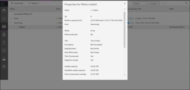
Figure 3-2 Array capacity monitoring with GUI
Example 3-3 Array capacity monitoring with CLI
IBM_FlashSystem:FS9100-ITSO:superuser>lsarray 0
mdisk_id 0
mdisk_name mdisk0
capacity 113.3TB
...
physical_capacity 24.50TB
physical_free_capacity 24.50TB
write_protected no
allocated_capacity 58.57TB
effective_used_capacity 22.59GB
•If the used physical capacity of the array reaches 99%, IBM FlashSystem raises event ID 1241: 1% physical space left for compressed array. This event is a call for immediate action.
To prevent running out of space, one or a combination of the following corrective actions must be taken:
– Add storage to the pool and wait while data is balanced between arrays by Easy Tier.
– Migrate volumes with extents on the managed disk that is running low on physical space to another storage pool or migrate extents from the array that is running low on physical space to other managed disks that have sufficient extents.
– Delete or migrate data from the volumes using a host that supports UNMAP commands. IBM FlashSystem will issue UNMAP to the array and space will be released.
For more information about out-of-space recovery, see this IBM Support web page.
•Arrays are most in danger of running out of space during a rebuild or when they are degraded. DRAID spare capacity, which is distributed across array drives, remains free during normal DRAID operation, thus reducing overall drive fullness. This means that if array capacity is 85% full, each array FCM is used for less than that due to spare space reserve. When DRAID is rebuilding this space becomes used.
After the rebuild is complete, the extra space is filled up and the drives can be truly full, resulting in high levels of write amplification and degraded performance. In the worst case (for example, if the array is more than 99% full before rebuild starts), there is a chance that the rebuild might cause a physical out-of-space condition.
3.3 General external storage considerations
IBM FlashSystem can virtualize external storage and make it available to the system. External back-end storage systems (or controllers in Spectrum Virtualize terminology) provide their logical volumes (LUs), which are detected by IBM FlashSystem as MDisks and can be used in storage pools.
This section covers aspects of planning and managing external storage virtualized by IBM FlashSystem.
External back-end storage can be connected to IBM FlashSystem with FC (SCSI) or iSCSI. NVMe-FC back-end attachment is not supported because it provides no performance benefits for IBM FlashSystem. For more information, see “NVMe protocol” on page 70.
On IBM FlashSystem 5010/5030 and FlashSystem 5015/5035, virtualization is allowed only for data migration. Therefore, this systems can be used to externally virtualize storage as an image mode device for the purposes of data migration, not for long term virtualization.
3.3.1 Storage controller path selection
When a managed disk (MDisk) logical unit (LU) is accessible through multiple storage system ports, the system ensures that all nodes that access this LU coordinate their activity and access the LU through the same storage system port.
An MDisk path that is presented to the storage system for all system nodes must meet the following criteria.
•The system node is a member of a storage system.
•The system node has Fibre Channel or iSCSI connections to the storage system port.
•The system node has successfully discovered the LU.
•The port selection process has not caused the system node to exclude access to the MDisk through the storage system port.
When the IBM FlashSystem node canisters select a set of ports to access the storage system, the two types of path selection described in the next sections are supported to access the MDisks. A type of path selection is determined by external system type and cannot be changed. To determine which algorithm is used for a specific back-end system, see System Storage Interoperaton Center (SSIC), as shown in Figure 3-3 on page 87.
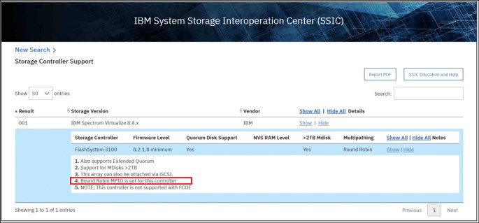
Figure 3-3 SSIC example
Round-robin path algorithm
With the round-robin path algorithm, each MDisk uses one path per target port per IBM FlashSystem node. This means that in cases of storage systems without a preferred controller such as XIV or DS8000, each MDisk uses all of the available FC ports of that storage controller.
With a round-robin compatible storage controller, there is no need to create as many volumes as there are storage FC ports anymore. Every volume, and therefore MDisk, uses all available IBM FlashSystem ports.
This configuration results in an significant increase in performance because the MDisk is no longer bound to one back-end FC port. Instead, it can issue I/Os to many back-end FC ports in parallel. Particularly, the sequential I/O within a single extent can benefit from this feature.
Additionally, the round-robin path selection improves resilience to certain storage system failures. For example, if one of the back-end storage system FC ports has performance problems, the I/O to MDisks is sent through other ports. Moreover, because I/Os to MDisks are sent through all back-end storage FC ports, the port failure can be detected more quickly.
|
Preferred practice: If you have a storage system that supports the round-robin path algorithm, you should zone as many FC ports as possible from the back-end storage controller. IBM FlashSystem supports up to 16 FC ports per storage controller. See your storage system documentation for FC port connection and zoning guidelines.
|
Example 3-4 shows a storage controller that supports round-robin path selection.
Example 3-4 Round robin enabled storage controller
IBM_FlashSystem:FS9100-ITSO:superuser>lsmdisk 4
id 4
name mdisk4
...
preferred_WWPN 20010002AA0244DA
active_WWPN many <<< Round Robin Enabled
MDisk group balanced and controller balanced
Although round-robin path selection provides optimized and balanced performance with minimum configuration required, there are storage systems that still require manual intervention to achieve the same goal.
With storage subsystems that use active-passive type systems, IBM FlashSystem accesses an MDisk LU through one of the ports on the preferred controller. To best use the back-end storage, it is important to make sure that the number of LUs that is created is a multiple of the connected FC ports and aggregate all LUs to a single MDisk group.
Example 3-5 shows a storage controller that supports MDisk group balanced path selection.
Example 3-5 MDisk group balanced path selection (no round robin enabled) storage controller
IBM_FlashSystem:FS9100-ITSO:superuser>lsmdisk 5
id 5
name mdisk5
...
preferred_WWPN
active_WWPN 20110002AC00C202 <<< indicates Mdisk group balancing
3.3.2 Guidelines for creating optimal backend configuration
Most of the backend controllers aggregate spinning or solid state drives into RAID arrays, then join arrays into pools. Logical volumes are created on those pools and provided to hosts. When connected to external backend storage, IBM FlashSystem acts as a host. It is important to create backend controller configuration that provides performance and resiliency, as IBM FlashSystem will rely on back-end storage when serving I/O to attached host systems.
If your back-end system has homogeneous storage, create the required number of RAID arrays (usually RAID 6 or RAID 10 are recommended) with equal number of drives. The type and geometry of an array depends on the back-end controller vendor’s recommendations. If your back-end controller can spread the load stripe across multiple arrays in a resource pool (for example, by striping), create a single pool and add all arrays there.
On back-end systems with mixed drives, create a separate resource pool for each drive technology. Keep the drive-technology type in mind, as you will need to assign the correct tier for an MDisk when it is used by IBM FlashSystem.
Create a set of fully allocated logical volumes from the back-end system storage pool (or pools). Each volume is detected as MDisk on IBM FlashSystem. The number of logical volumes to create depends the type of drives, used by your back-end controller.
Back-end controller with spinning drives
If your back-end is using spinning drives, volume number calculation must be based on a queue depth. Queue depth is the number of outstanding I/O requests of a device.
For optimal performance, spinning drives need 8-10 concurrent I/O at the device, and this doesn’t change with drive rotation speed. Make sure in a highly loaded system, that any given IBM FlashSystem MDisk can queue up approximately 8 I/O per back-end system drive.
IBM FlashSystem queue depth per MDisk is approximately 60. The exact maximum seen on a real system might vary depending on the circumstances. However, for the purpose of this calculation it does not matter.
The queue depth per MDisk number leads to the HDD Rule of 8. According to this rule, to achieve 8 I/O per drive and with queue depth 60 per MDisk from IBM FlashSystem, a back-end array with 60/8 = 7.5 that is approximately equal to eight physical drives is optimal, or we need one logical volume per every eight drives in an array.
|
Example: The back-end controller to be virtualized is IBM Storwize V5030 with 64 NL-SAS 8 TB drives.
The system is homogeneous. According to recommendations that are described in 3.2.2, “Array considerations” on page 80, create a single DRAID6 array at IBM Storwize and include it in a storage pool. By using the HDD rule of 8, we want 64/8 = 8 MDisks; therefore, create eight volumes from a pool to present to IBM FlashSystem and assign them to the nearline tier.
|
All-flash back-end controllers
For All-flash controllers, the considerations are more of I/O distribution across IBM FlashSystem ports and processing threads, than of queue depth per drive. Since most All-flash arrays that are put behind virtualizer have high I/O capabilities, make sure that IBM FlashSystem is given the optimal chance to spread the load and evenly make use of its internal resources, so queue depths are of less a concern here (because of the lower latency per I/O).
For all-flash back-end arrays, IBM recommends creating 32 logical volumes from the array capacity, as it allows to keep the queue depths high enough and spreads the work across the virtualizer resources. For smaller setups with a low number of solid state drives this number can be reduced to 16 logical volumes (which results in 16 MDisks) or even 8 volumes.
|
Example: Back-end controllers to be virtualized are IBM FlashSystem 5035 with 24 Tier1 7.6 TB drives and IBM FlashSystem 9200. The virtualizer needs a pool with two storage tiers:
•On IBM FlashSystem 5035, create a single DRAID6 array and add it to a storage pool. Using all-flash rule, we must create 32 volumes to present as MDisks. However, because it is small setup, we can reduce the number of volumes to 16.
•On IBM FlashSystem 9200, join all micro-latency modules into a RAID5 array and add it to a storage pool. Because FlashSystem 9200 is Tier0 solution, use all-flash rule, and create 32 volumes to present as MDisks.
•On virtualizer, add 16 MDisks from IBM FlashSystem 5035 as Tier1 flash, and 32 MDisks as Tier0 flash, to a single multi-tier pool.
|
Large setup considerations
For controllers like IBM DS8000 and XIV, you can use all-flash rule of 32. However, with installations involving this type of back-end controllers, it might be necessary to consider a maximum queue depth per back-end controller port, which is set to 1000 for most supported high-end storage systems.
With high-end controllers, queue depth per MDisk can be calculated by using the following formula:
Q = ((P x C) / N) / M
Where:
Q Calculated queue depth for each MDisk.
P Number of back-end controller host ports (unique WWPNs) that are zoned to IBM FlashSystem (minimum is 2 and maximum is 16).
C Maximum queue depth per WWPN, which is 1000 for controllers, such as XIV or DS8000.
N Number of nodes in the IBM FlashSystem cluster (2, 4, 6, or 8).
M Number of volumes that are presented by back-end controller and detected as MDisks.
For a result of Q = 60, calculate the number of volumes that is needed to create as M = (P x C) / (N x Q), which can be simplified to M = (16 x P) / N.
|
Example: A 4-node IBM FlashSystem 9200 is used with 12 host ports on the IBM XIV System.
By using the previous formula, we must create M = (16 x 12) / 4 = 48 volumes on IBM XIV to obtain a balanced high-performing configuration.
|
3.3.3 Considerations for compressing and deduplicating back-end
IBM FlashSystem supports over-provisioning on selected back-end controllers. This means that if back-end storage performs data deduplication or data compression on LUs provisioned from it, the LUs still can be used as external MDisks on IBM FlashSystem.
The implementation steps for thin-provisioned MDisks are the same as for fully allocated storage controllers. Extreme caution should be used when planning capacity for such configurations.
The IBM FlashSystem detects:
•If the MDisk is thin-provisioned.
•The total physical capacity of the MDisk.
•The used and remaining physical capacity of the MDisk.
•Whether unmap commands are supported by the back-end. By sending SCSI unmap commands to thin-provisioned MDisks, the system marks data that is no longer in use. Then, the garbage-collection processes on the back-end can free unused capacity and reallocate it to free space.
Using an appropriate compression and or data deduplication ratio is key to achieving a stable environment. If you are not sure about the real compression or data deduplication ratio, contact your IBM technical sales representative to obtain more information.
The nominal capacity from a compression and deduplication enabled storage system is not fixed and it varies based on the nature of the data. Always use a conservative data reduction ratio for the initial configuration.
Using the suitable ratio for capacity assignment can cause an out of space situation. If the MDisks do not provide enough capacity, IBM FlashSystem disables access to all the volumes in the storage pool.
|
Example: This example includes the following assumptions:
•Assumption 1: Sizing is performed with an optimistic 5:1 rate
•Assumption 2: Real rate is 3:1
Therefore:
•Physical Capacity: 20 TB
•Calculated capacity: 20 TB x 5 = 100 TB
•The volume that is assigned from the compression- or deduplication-enabled storage subsystem to the IBM SAN Volume Controller or IBM Storwize is 100 TB
•Real usable capacity: 20 TB x 3 = 60 TB
If the hosts attempt to write more than 60 TB data to the storage pool, the storage subsystem cannot provide any more capacity. Also, all volumes that are used as IBM Spectrum Virtualize or Storwize Managed Disks and all related pools go offline.
|
Thin-provisioned back-end storage must be carefully monitored. It is necessary to set up capacity alerts to be aware of the real remaining physical capacity.
Also, the best practice is to have an emergency plan and know the steps to recover from an “Out Of Physical Space” situation on the back-end controller. The plan must be prepared during the initial implementation phase.
3.4 Controller-specific considerations
This section discusses implementation-specific information that is related to different supported back-end systems. For more information about general requirements, see this IBM Documentation web page.
3.4.1 Considerations for DS8000 series
In this section, we discuss considerations for the DS800 series.
Interaction between DS8000 and IBM FlashSystem
It is important to know DS8000 drive virtualization process, which is the process of preparing physical drives for storing data that belongs to a volume that is used by a host. In this case, the host is the IBM FlashSystem.
In this regard, the basis for virtualization begins with the physical drives of DS8000, which are mounted in storage enclosures. Virtualization builds upon the physical drives as a series of layers:
•Array sites
•Arrays
•Ranks
•Extent pools
•Logical volumes
•Logical subsystems
Array sites are the building blocks that are used to define arrays, which are data storage systems for block-based, file-based, or object based storage. Instead of storing data on a server, storage arrays use multiple drives that are managed by a central management and can store a huge amount of data.
In general terms, eight identical drives that have the same capacity, speed, and drive class comprise the array site. When an array is created, the RAID level, array type, and array configuration are defined. RAID 5, RAID 6, and RAID 10 levels are supported.
|
Important: Normally the RAID 6 is highly preferred, and is the default while using the Data Storage Graphical Interface (DS GUI). As with large drives in particular, the RAID rebuild times (after one drive failure) become larger. Using RAID 6 reduces the danger of data loss due to a double-RAID failure. For more information, see this IBM Documentation web page.
|
A rank, which is a logical representation for the physical array, is relevant for IBM FlashSystem because of the creation of a fixed block (FB) pool for each array that you want to virtualize. Ranks in DS8000 are defined in a one-to-one relationship to arrays. It is for this reason that a rank is defined as using only one array.
A fixed-block rank features one of the following extent sizes:
•1 GiB, which is a large extent
•16 MiB, which is a small extent
An extent pool or storage pool in DS8000 is a logical construct to add the extents from a set of ranks, forming a domain for extent allocation to a logical volume.
In synthesis, a logical volume consists of a set of extents from one extent pool or storage pool. DS8900F supports up to 65,280 logical volumes.
A logical volume that is composed of fix block extents is called logical unit number (LUN). A fixed-block LUN consists of one or more 1 GiB (large) extents, or one or more 16 MiB (small) extents from one FB extent pool. A LUN is not allowed to cross extent pools. However, a LUN can have extents from multiple ranks within the same extent pool.
|
Important: DS8000 Copy Services does not support FB logical volumes larger than 2 TiB. Therefore, you cannot create a LUN that is larger than 2 TiB if you want to use Copy Services for the LUN, unless the LUN is integrated as Managed Disks in an IBM FlashSystem. Use IBM Spectrum Virtualize Copy Services instead. Based on the considerations, the maximum LUN sizes to create at DS8900F and present to IBM FlashSystem are as follows:
•16 TB LUN with large extents (1 GiB)
•16 TB LUN with small extent (16 MiB) for DS8880F with version or edition R8.5 or later, and for DS8900F R9.0 or later.
|
Logical subsystems (or LSS) are another logical construct, and mostly used in conjunction with fixed-block volumes. Thus, a maximum of 255 LSSs can exist on DS8900F. For more information, see this IBM Documentation web page.
The concepts of virtualization of DS8900F for IBM FlashSystem are schematically shown in Figure 3-4.
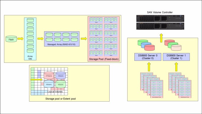
Figure 3-4 DS8900 virtualization concepts focus to IBM FlashSystem
Connectivity considerations
The number of DS8000 ports to be used is at least eight. With large and workload intensive configurations, consider using more ports, up to 16, which is the maximum supported by IBM FlashSystem.
Generally, use ports from different host adapters and, if possible, from different I/O enclosures. This configuration is also important because during a DS8000 LIC update, a host adapter port might need to be taken offline. This configuration allows the IBM FlashSystem I/O to survive a hardware failure on any component on the SAN path.
For more information about SAN preferred practices and connectivity, see Chapter 2, “Connecting IBM Spectrum Virtualize and IBM Storwize in storage area networks” on page 37.
Defining storage
To optimize the DS8000 resource utilization, use the following guidelines:
•Distribute capacity and workload across device adapter pairs.
•Balance the ranks and extent pools between the two DS8000 internal servers to support the corresponding workloads on them.
•Spread the logical volume workload across the DS8000 internal servers by allocating the volumes equally on rank groups 0 and 1.
•Use as many disks as possible. Avoid idle disks, even if all storage capacity is not to be used initially.
•Consider the use of multi-rank extent pools.
•Stripe your logical volume across several ranks, which is the default for multi-rank extent pools.
Balancing workload across DS8000 series controllers
When you configure storage on the DS8000 series disk storage subsystem, ensure that ranks on a device adapter (DA) pair are evenly balanced between odd and even extent pools. If you do not ensure that the ranks are balanced, uneven device adapter loading can cause a considerable performance degradation.
The DS8000 series controllers assign server (controller) affinity to ranks when they are added to an extent pool. Ranks that belong to an even-numbered extent pool have an affinity to Server 0, and ranks that belong to an odd-numbered extent pool have an affinity to Server 1.
Figure 3-5 shows an example of a configuration that results in a 50% reduction in available bandwidth. Notice how arrays on each of the DA pairs are accessed only by one of the adapters. In this case, all ranks on DA pair 0 are added to even-numbered extent pools, which means that they all have an affinity to Server 0. Therefore, the adapter in Server 1 is sitting idle. Because this condition is true for all four DA pairs, only half of the adapters are actively performing work. This condition can also occur on a subset of the configured DA pairs.
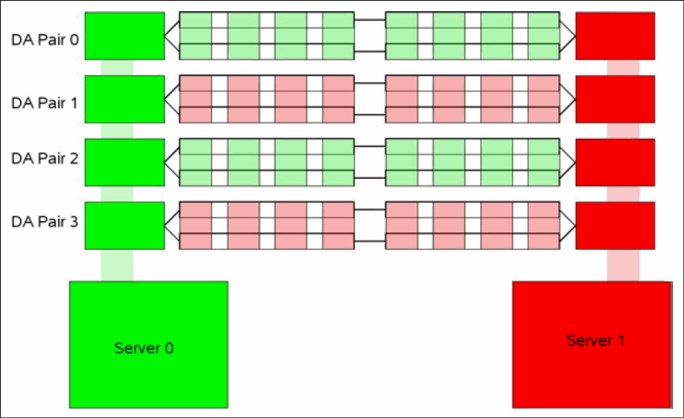
Figure 3-5 DA pair reduced bandwidth configuration
Example 3-6 on page 95 shows the invalid configuration, as depicted in the CLI output of the lsarray and lsrank commands. The arrays that are on the same DA pair contain the same group number (0 or 1), meaning that they have affinity to the same DS8000 series server. Here, Server 0 is represented by Group 0, and server1 is represented by group1.
As an example of this situation, consider arrays A0 and A4, which are attached to DA pair 0. In this example, both arrays are added to an even-numbered extent pool (P0 and P4) so that both ranks have affinity to Server 0 (represented by Group 0), which leaves the DA in Server 1 idle.
Example 3-6 Command output for the lsarray and lsrank commands
dscli> lsarray -l
Date/Time: Oct 20, 2016 12:20:23 AM CEST IBM DSCLI Version: 7.8.1.62 DS: IBM.2107-75L2321
Array State Data RAID type arsite Rank DA Pair DDMcap(10^9B) diskclass
===================================================================================
A0 Assign Normal 5 (6+P+S) S1 R0 0 146.0 ENT
A1 Assign Normal 5 (6+P+S) S9 R1 1 146.0 ENT
A2 Assign Normal 5 (6+P+S) S17 R2 2 146.0 ENT
A3 Assign Normal 5 (6+P+S) S25 R3 3 146.0 ENT
A4 Assign Normal 5 (6+P+S) S2 R4 0 146.0 ENT
A5 Assign Normal 5 (6+P+S) S10 R5 1 146.0 ENT
A6 Assign Normal 5 (6+P+S) S18 R6 2 146.0 ENT
A7 Assign Normal 5 (6+P+S) S26 R7 3 146.0 ENT
dscli> lsrank -l
Date/Time: Oct 20, 2016 12:22:05 AM CEST IBM DSCLI Version: 7.8.1.62 DS: IBM.2107-75L2321
ID Group State datastate Array RAIDtype extpoolID extpoolnam stgtype exts usedexts
======================================================================================
R0 0 Normal Normal A0 5 P0 extpool0 fb 779 779
R1 1 Normal Normal A1 5 P1 extpool1 fb 779 779
R2 0 Normal Normal A2 5 P2 extpool2 fb 779 779
R3 1 Normal Normal A3 5 P3 extpool3 fb 779 779
R4 0 Normal Normal A4 5 P4 extpool4 fb 779 779
R5 1 Normal Normal A5 5 P5 extpool5 fb 779 779
R6 0 Normal Normal A6 5 P6 extpool6 fb 779 779
R7 1 Normal Normal A7 5 P7 extpool7 fb 779 779
Figure 3-6 shows a configuration that balances the workload across all four DA pairs.
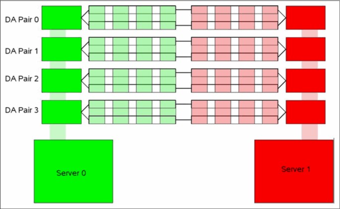
Figure 3-6 DA pair correct configuration
Figure 3-7 shows a correct configuration, as depicted in the CLI output of the lsarray and lsrank commands. Notice that the output shows that this configuration balances the workload across all four DA pairs with an even balance between odd and even extent pools. The arrays that are on the same DA pair are split between groups 0 and 1.

Figure 3-7 The lsarray and lsrank command output
DS8000 series ranks to extent pools mapping
In the DS8000 architecture, extent pools are used to manage one or more ranks. An extent pool is visible to both processor complexes in the DS8000 storage system, but it is directly managed by only one of them. You must define a minimum of two extent pools with one extent pool that is created for each processor complex to fully use the resources. You can use the following approaches:
•One-to-one approach: One rank per extent pool configuration.
With the one-to-one approach, DS8000 is formatted in 1:1 assignment between ranks and extent pools. This configuration disables any DS8000 storage-pool striping or auto-rebalancing activity, if they were enabled. You can create one or two volumes in each extent pool exclusively on one rank only and put all of those volumes into one IBM FlashSystem storage pool. IBM FlashSystem stripes across all of these volumes and balances the load across the RAID ranks by that method. No more than two volumes per rank are needed with this approach. So, the rank size determines the volume size.
Often, systems are configured with at least two storage pools:
– One (or two) that contain MDisks of all the 6+P RAID 5 ranks of the DS8000 storage system.
– One (or more) that contain the slightly larger 7+P RAID 5 ranks.
This approach maintains equal load balancing across all ranks when the IBM FlashSystem striping occurs because each MDisk in a storage pool is the same size.
The IBM FlashSystem extent size is the stripe size that is used to stripe across all these single-rank MDisks.
This approach delivered good performance and has its justifications. However, it also has a few minor drawbacks:
– A natural skew, such as a small file of a few hundred KiB that is heavily accessed.
– When you have more than two volumes from one rank, but not as many IBM FlashSystem storage pools, the system might start striping across many entities that are effectively in the same rank, depending on the storage pool layout. Such striping should be avoided.
An advantage of this approach is that it delivers more options for fault isolation and control over where a certain volume and extent are located.
•Many-to-one approach: Multi-rank extent pool configuration.
A more modern approach is to create a few DS8000 extent pools; for example, two DS8000 extent pools. Use DS8000 storage pool striping or automated Easy Tier rebalancing to help prevent overloading individual ranks.
Create at least two extent pools for each tier to balance the extent pools by Tier and Controller affinity. Mixing different tiers on the same extent pool is effective only when Easy Tier is activated on the DS8000 pools. However, when virtualized, tier management has more advantages when handled by the IBM FlashSystem.
For more information about choosing the level on which to run Easy Tier, see “Monitoring Easy Tier using the GUI” on page 191.
You need only one volume size with this multi-rank approach because plenty of space is available in each large DS8000 extent pool. As mentioned previously, the maximum number of back-end storage ports to be presented to the IBM FlashSystem is 16. Each port represents a path to the IBM FlashSystem. Therefore, when sizing the number of LUN/MDisks to be presented to the IBM FlashSystem, the suggestion is to present least between two and four volumes per path. So using the maximum of 16 paths, create 32, 48, or 64 DS8000 volumes, and for this configuration IBM FlashSystem maintains a good queue depth.
To maintain the highest flexibility and for easier management, large DS8000 extent pools are beneficial. However, if the DS8000 installation is dedicated to shared-nothing environments, such as Oracle ASM, IBM DB2® warehouses, or General Parallel File System (GPFS), use the single-rank extent pools.
LUN masking
For a storage controller, all IBM FlashSystem nodes must detect the same set of LUs from all target ports that logged in. If target ports are visible to the nodes or canisters that do not have the same set of LUs assigned, IBM FlashSystem treats this situation as an error condition and generates error code 1625.
You must validate the LUN masking from the storage controller and then confirm the correct path count from within the IBM FlashSystem.
The DS8000 series controllers perform LUN masking that is based on the volume group. Example 3-7 shows the output of the showvolgrp command for volume group (V0), which contains 16 LUNs that are being presented to a two-node IBM FlashSystem cluster.
Example 3-7 Output of the showvolgrp command
dscli> showvolgrp V0
Date/Time: Oct 20, 2016 10:33:23 AM BRT IBM DSCLI Version: 7.8.1.62 DS: IBM.2107-75FPX81
Name ITSO_SVC
ID V0
Type SCSI Mask
Vols 1001 1002 1003 1004 1005 1006 1007 1008 1101 1102 1103 1104 1105 1106 1107 1108
Example 3-8 shows output for the lshostconnect command from the DS8000 series. In this example, four ports of the two-node cluster are assigned to the same volume group (V0) and, therefore, are assigned to the same four LUNs.
Example 3-8 Output for the lshostconnect command
dscli> lshostconnect -volgrp v0
Date/Time: Oct 22, 2016 10:45:23 AM BRT IBM DSCLI Version: 7.8.1.62 DS: IBM.2107-75FPX81
Name ID WWPN HostType Profile portgrp volgrpID ESSIOport
=============================================================================================
ITSO_SVC_N1C1P4 0001 500507680C145232 SVC San Volume Controller 1 V0 all
ITSO_SVC_N1C2P3 0002 500507680C235232 SVC San Volume Controller 1 V0 all
ITSO_SVC_N2C1P4 0003 500507680C145231 SVC San Volume Controller 1 V0 all
ITSO_SVC_N2C2P3 0004 500507680C235231 SVC San Volume Controller 1 V0 all
From Example 3-8 you can see that only the IBM FlashSystem WWPNs are assigned to V0.
|
Attention: Data corruption can occur if the same LUN is assigned to IBM FlashSystem nodes and other devices, such as hosts attached to DS8000.
|
Next, you see how the IBM FlashSystem detects these LUNs if the zoning is properly configured. The Managed Disk Link Count (mdisk_link_count) represents the total number of MDisks that are presented to the IBM FlashSystem cluster by that specific controller.
Example 3-9 shows the general details of the output storage controller by using the system CLI.
Example 3-9 Output of the lscontroller command
IBM_FlashSystem:FS9100-ITSO:superuser>svcinfo lscontroller DS8K75FPX81
id 1
controller_name DS8K75FPX81
WWNN 5005076305FFC74C
mdisk_link_count 16
max_mdisk_link_count 16
degraded no
vendor_id IBM
product_id_low 2107900
...
WWPN 500507630500C74C
path_count 16
max_path_count 16
WWPN 500507630508C74C
path_count 16
max_path_count 16
IBM FlashSystem MDisks and storage pool considerations
Recommended practice is to create a single IBM FlashSystem storage pool per DS8900F system. This provides simplicity of management, and best overall performance.
An example of the preferred configuration is shown in Figure 3-8 on page 99. Four storage pools or extent pools (one even and one odd) of DS8900F are joined into one IBM FlashSystem storage pool.

Figure 3-8 Four DS8900F extent pools as one IBM FlashSystem storage pool
To determine how many logical volumes must be created to present to IBM FlashSystem as MDisks, see 3.3.2, “Guidelines for creating optimal backend configuration” on page 88.
3.4.2 Considerations for IBM XIV Storage System
The XIV Gen3 volumes can be provisioned to IBM FlashSystem by way of iSCSI and FC. However, it is preferred that you implement FC attachment for performance and stability considerations, unless a dedicated IP infrastructure for storage is available.
Host options and settings for XIV systems
You must use specific settings to identify IBM FlashSystem systems as hosts to XIV systems. An XIV node within an XIV system is a single WWPN. An XIV node is considered to be a single SCSI target. Each host object that is created within the XIV System must be associated with the same LUN map.
From an IBM FlashSystem perspective, an XIV type 281x controller can consist of more than one WWPN. However, all are placed under one worldwide node number (WWNN) that identifies the entire XIV system.
Creating a host object for IBM FlashSystem for an IBM XIV
A single host object with all WWPNs of IBM FlashSystem nodes can be created when implementing IBM XIV. This technique makes the host configuration easier to configure. However, the ideal host definition is to consider each node IBM FlashSystem as a host object, and create a cluster object to include all nodes or canisters.
When implemented in this manner, statistical metrics are more effective because performance can be collected and analyzed on IBM FlashSystem node level.
A detailed procedure to create a host on XIV is available in IBM XIV Gen3 with IBM System Storage SAN Volume Controller and Storwize V7000, REDP-5063.
Volume considerations
As modular storage, XIV storage can be available in a minimum of six modules and up to a maximum of 15 modules in a configuration. Each additional module added to the configuration increases the XIV capacity, CPU, memory, and connectivity.
As of this writing, the XIV system supports the following configurations:
•28 - 81 TB when 1-TB drives are used
•55 - 161 TB when 2-TB disks are used
•84 - 243 TB when 3-TB disks are used
•112 - 325 TB when 4-TB disks are used
•169 - 489 TB when 6-TB disks are used
Figure 3-9 shows how XIV configurations vary according to the number of modules that are on the system.

Figure 3-9 XIV rack configuration: 281x-214
Although XIV has its own queue depth characteristics for direct host attachment, the best practices that are described in 3.3.2, “Guidelines for creating optimal backend configuration” on page 88 are preferred when you virtualize XIV with IBM Spectrum Virtualize.
Table 3-6 lists s the suggested volume sizes and quantities for IBM FlashSystem on the XIV systems with different drive capacities.
Table 3-6 XIV minimum volume size and quantity recommendations
|
Modules
|
XIV host ports
|
Volume size (GB) 1 TB drives
|
Volume size (GB) 2 TB drives
|
Volume size (GB) 3 TB drives
|
Volume size (GB) 4 TB drives
|
Volume size (GB)
6 TB drives
|
Volume quantity
|
Volumes to XIV host ports
|
|
06
|
04
|
1600
|
3201
|
4852
|
6401
|
9791
|
17
|
4.3
|
|
09
|
08
|
1600
|
3201
|
4852
|
6401
|
9791
|
27
|
3.4
|
|
10
|
08
|
1600
|
3201
|
4852
|
6401
|
9791
|
31
|
3.9
|
|
11
|
10
|
1600
|
3201
|
4852
|
6401
|
9791
|
34
|
3.4
|
|
12
|
10
|
1600
|
3201
|
4852
|
6401
|
9791
|
39
|
3.9
|
|
13
|
12
|
1600
|
3201
|
4852
|
6401
|
9791
|
41
|
3.4
|
|
14
|
12
|
1600
|
3201
|
4852
|
6401
|
9791
|
46
|
3.8
|
|
15
|
12
|
1600
|
3201
|
4852
|
6401
|
9791
|
50
|
4.2
|
Other considerations
Consider the following restrictions when using the XIV system as back-end storage for the IBM FlashSystem:
•Volume mapping
When mapping a volume, you must use the same LUN ID to all IBM FlashSystem nodes. Therefore, map the volumes to the cluster, not to individual nodes.
•XIV Storage pools
When creating an XIV storage pool, define the Snapshot Size as zero (0). Snapshot space does not need to be reserved, because it is not recommended that you use XIV snapshots on LUNs mapped as MDisks. The snapshot functions should be used on IBM FlashSystem level.
As all LUNs on a single XIV system share performance and capacity characteristics, use a single IBM FlashSystem storage pool for a single XIV system.
•Thin provisioning
XIV thin provisioning pools are not supported by IBM FlashSystem. Instead, you must use a regular pool.
•Copy functions for XIV models
You cannot use advanced copy functions, such as taking a snapshot and remote mirroring, for XIV models with disks that are managed by the IBM FlashSystem.
For more information about configuration of XIV behind IBM FlashSystem, see IBM XIV Gen3 with IBM System Storage SAN Volume Controller and Storwize V7000, REDP-5063.
3.4.3 Considerations for IBM FlashSystem A9000/A9000R
IBM FlashSystem A9000 and IBM FlashSystem A9000R use industry-leading data-reduction technology that combines inline, real-time pattern matching and removal, data deduplication, and compression. Compression also uses hardware cards inside each grid controller. Compression can easily provide a 2:1 data reduction saving rate on its own, effectively doubling the system storage capacity. Combined with pattern removal and data deduplication services, IBM FlashSystem A9000/A9000R can easily yield an effective data capacity of five times the original usable physical capacity.
Deduplication can be implemented on the IBM FlashSystem by attaching an IBM FlashSystem A9000/A9000R as external storage instead of using IBM Spectrum Virtualize DRP-level deduplication.
There are several considerations when you are attaching an IBM FlashSystem A9000/A9000R system as a back-end controller.
Volume considerations
IBM FlashSystem A9000/A9000R designates resources to data reduction, and as this designation is always on, it is strongly advised that data reduction be done only in the IBM FlashSystem A9000/A9000R and not in the Spectrum Virtualize cluster. Otherwise, as IBM FlashSystem A9000/A9000R tries to reduce the data, unnecessary additional latency occurs.
Estimated data reduction is important because that helps determine volume size. Always try to use a conservative data-reduction ratio when attaching A9000/A9000R, because the storage pool will go offline if the back-end storage runs out of capacity.
To determine the controller volume size, complete the following tasks:
•Calculate effective capacity: reduce measured-data reduction ratio (for example, if the data reduction estimation tool provides a ratio of 4:1, use 3.5:1 for calculations) and multiply it to determine physical capacity.
•Volume size is equal to effective capacity that is divided by the number of ports taken twice (effective capacity/path*2).
The remaining usable capacity can be added to the storage pool after the system reaches a stable date reduction ratio.
Table 3-7 Host connections for A9000
|
Number of controllers
|
Total FC ports available
|
Total ports that are connected to IBM SAN Volume Controller
|
Connected ports
|
|
3
|
12
|
6
|
All controllers, ports 1 and 3
|
Table 3-8 Host connections for A9000R
|
Grid element
|
Number of controllers
|
Total FC ports available
|
Total ports that are connected to IBM SAN Volume Controller
|
Connected ports
|
|
2
|
04
|
16
|
08
|
All controllers, ports 1 and 3
|
|
3
|
06
|
24
|
12
|
All controllers, ports 1 and 3
|
|
4
|
08
|
32
|
08
|
Controllers 1 - 4, port 1 Controllers 5 - 8, port 3
|
|
5
|
10
|
40
|
10
|
Controllers 1 - 5, port 1 Controllers 6 - 10, port 3
|
|
6
|
12
|
48
|
12
|
Controllers 1 - 6, port 1 Controllers 7 - 12, port 3
|
It is important not to run out of hard capacity on the back-end storage because doing so takes the storage pool offline. It is important to closely monitor the FlashSystem A9000/A9000R. If you start to run out of space, you can use the migration functions of Spectrum Virtualize to move data to another storage system, as described in the examples next.
|
Examples: Consider the following examples:
•FlashSystem A9000 with 57 TB of usable capacity, or 300 TB of effective capacity, at the standard 5.26:1 data efficiency ratio.
We ran the data reduction tool on a good representative sample of the volumes that we will be virtualizing. We know that we have a data reduction ratio of 4.2:1 and for extra safety, use 4:1 for further calculations. The use of 4 x 57 gives you 228 TB. Divide this result by 12 (six paths x 2), and you get 19 TB per volume.
•A five-grid element FlashSystem A9000R that uses 29 TB Flash enclosures has a total usable capacity of 145 TB.
We are use 10 paths and have not run any of the estimation tools on the data. However, we know that the host is not compressing the data. We assume a compression ratio of 2:1, 2 x 145 gives 290, and divided by 20 gives 14.5 TB per volume. In this case, if we see that we are getting a much better data reduction ratio than we planned for, we can always create volumes and make them available to IBM Spectrum Virtualize.
|
The biggest concern about the number of volumes is to ensure there is adequate queue depth. Given that the maximum volume size on the FlashSystem A9000/A9000R is 1 PB and you are ensuring two volumes per path, you should be able to create a small number of larger volumes and still have good queue depth and not have numerous volumes to manage.
Other considerations
Spectrum Virtualize is able to detect that the IBM FlashSystem A9000 controller is using deduplication technology and show that the Deduplication attribute of the managed disk is Active.
Deduplication status is important because it allows IBM Spectrum Virtualize to enforce the following restrictions:
•Storage pools with deduplicated MDisks should only contain MDisks from the same IBM FlashSystem A9000 or IBM FlashSystem A9000R storage controller.
•Deduplicated MDisks cannot be mixed in an Easy Tier enabled storage pool.
3.4.4 Considerations for FlashSystem 5000, 5100, 5200, 7200, 9100, and 9200
Recommendations that are discussed in this section apply to a solution with IBM FlashSystem family or IBM Storwize family system that is virtualized by another IBM FlashSystem family system.
Connectivity considerations
It is expected that NPIV is enabled on both systems: the system that is virtualizing storage, and the system that works as a back-end. Zone “host” or “virtual” WWPNs of the back-end system to physical WWPNs of the front-end, or virtualizing system.
For more information about SAN and zoning preferred practices, see Chapter 2, “Connecting IBM Spectrum Virtualize and IBM Storwize in storage area networks” on page 37.
System layers
Spectrum Virtualize systems have a concept of system layers. There are two layers - storage and replication. Systems that are configured into storage layer can work as a back-end storage. Systems that are configured into replication layer, can virtualize another IBM FlashSystem clusters and use them as back-end controllers.
Systems that are configured with the same layer can be replication partners. Systems in the different layers cannot.
By default, IBM FlashSystem is configured to storage layer. The system layer on IBM FlashSystem can be switched. IBM SAN Volume Controller is configured to replication layer, and it cannot be changed on IBM SAN Volume Controller.
For more information and instructions and limitations, see this IBM Documentation web page.
Automatic configuration
IBM FlashSystem family systems that run code version 8.3x and above can be automatically configured for optimal performance as a back-end storage behind IBM SAN Volume Controller.
An automatic configuration wizard must be used on a system where volumes, pools, and host objects are not configured. Wizard will configure internal storage devices, create volumes and map the to the host object, representing IBM SAN Volume Controller.
Array and disk pool considerations
The back-end IBM FlashSystem family system can have a hybrid configuration, containing FlashCore Modules and SSD drives, or SSDs and spinning drives.
Internal storage attached to the back-end system needs to be joined into RAID arrays. You might need one or more DRAID6 arrays, depending on the number and the type of available drives. For RAID recommendations, see 3.2.2, “Array considerations” on page 80.
Consider creating a separate disk pool for each type (tier) of storage and use the Easy Tier function on a front-end system. Front-end FlashSystem family systems cannot monitor Easy Tier activity of the back-end storage.
If Easy Tier is enabled on front- and back-end systems, they independently rebalance the hot areas according to their own heat map. This process causes a rebalance over a rebalance. Such a situation can eliminate the performance benefits of extent reallocation. For this reason, Easy Tier must be enabled only on one level (preferably the front-end).
For more information about recommendations about Easy Tier with external storage, see Chapter 4, “Planning storage pools” on page 111.
For most use cases, standard pools are preferred to data-reduction pools on the back-end storage. If planned, the front-end will perform reduction. Data reduction on both levels is not recommended as it adds processing overhead and does not result in capacity savings.
If Easy Tier is disabled on the backend, as advised here, back-end FlashSystem pool extent size is not a performance concern.
SCSI Unmap considerations
When virtualized, IBM FlashSystem treats “virtualizer” system as a host. By default, host SCSI UNMAP support is enabled on IBM FlashSystem 9100 and FlashSystem 9200, and disabled on other platforms.
Consider enabling host Unmap support to achieve better capacity management if the system that is going to be virtualized meets the following qualifications:
•Contains FCMs
•Is Flash-only (no spinning drives)
Consider leaving host Unmap disabled to protect virtualized system from being over-loaded if you are going to virtualize a hybrid system, and storage to be virtualized uses spinning disks.
To switch host Unmap support on or off, use the chssystem CLI command. For more information, see this IBM Documentation web page.
Volume considerations
Volumes in IBM FlashSystem can be created as striped or sequential. The general rule is to create striped volumes. Volumes on back-end system must be fully allocated.
To determine a number of volumes to create on back-end IBM FlashSystem to provide a virtualizer as MDisks, see the general rules provided in 3.3.2, “Guidelines for creating optimal backend configuration” on page 88. When virtualizing back-end with spinning drives, perform queue depth calculations. For all flash solutions, create 32 volumes from the available pool capacity, which can be reduced to 16 or even 8 for small arrays (for example, if you have 16 or less flash drives in a back-end pool). For FCM arrays, the number of volumes is also governed by load distribution. 32 volumes out of a pool with an FCM array are recommended.
When choosing volume size, consider which system (front-end or back-end) performs the compression. If data is compressed and deduplicated on the front-end IBM FlashSystem (or “virtualizer”), FCMs cannot compress it further, which results in a 1:1 compression ratio.
Therefore, the back-end volume size is calculated from the pool physical capacity that is divided by the number of volumes (16 or more).
|
Example: FlashSystem 9200 with 24 x 19.2 TB modules.
This configuration provides raw disk capacity of 460 TB, with 10+P+Q DRAID6 and one distributed spare, and the physical array capacity is 365 TB or 332 TiB.
Because it is not recommended to provision more than 85% of a physical flash, we have 282 TiB. Because we do not expect any compression on FCM (the backend is getting data that is compressed by upper levels), we provision storage to upper level assuming a 1:1 compression, which means we create 32 volumes 282 TiB / 32 = 8.8 TiB each.
|
If the front-end system is not compressing data, space savings are achieved with FCM hardware compression. Use compression-estimation tools to determine the expected compression ratio and use a smaller ratio for further calculations (for example, if you expect 4.5:1 compression, use 4.3:1). Determine the volume size by using the calculated effective pool capacity.
|
Example: IBM FlashSystem 7200 with 12 x 9.6 TB modules.
This configuration provides raw disk capacity of 115 TB, with 9+P+Q DRAID6 and one distributed spare. The physical capacity is 85 TB or 78 TiB.
Because it is not recommended to provision more than 85% of a physical flash, we have 66 TiB. Compresstimator shows that we can achieve 3.2:1 compression ratio, decreasing in and assuming 3:1, we have 66 TiB x 3 = 198 TiB of effective capacity.
Create 16 volumes, 198TiB / 16 = 12.4 TiB each. If the compression ratio is higher than expected, we can create and provision more volumes to the frontend.
|
3.4.5 IBM FlashSystem 900 considerations
The main advantage of integrating FlashSystem 900 with IBM Spectrum Virtualize is to combine the extreme performance of IBM FlashSystem 900 with the Spectrum Virtualize enterprise-class solution such as tiering, volume mirroring, deduplication, and copy services.
When you configure the IBM FlashSystem 900 as a backend for Spectrum Virtualize family systems, you must remember the considerations that are described in this section.
Defining storage
IBM FlashSystem 900 supports up to 12 IBM MicroLatency® modules. IBM MicroLatency modules are installed in the IBM FlashSystem 900 based on the following configuration guidelines:
•A minimum of four MicroLatency modules must be installed in the system. RAID 5 is the only supported configuration of the IBM FlashSystem 900.
•The system supports configurations of 4, 6, 8, 10, and 12 MicroLatency modules in RAID 5.
•All MicroLatency modules that are installed in the enclosure must be identical in capacity and type.
•For optimal airflow and cooling, if fewer than 12 MicroLatency modules are installed in the enclosure, populate the module bays beginning in the center of the slots and adding on either side until all 12 slots are populated.
The array configuration is performed during system setup. The system automatically creates MDisk/arrays and defines the RAID settings based on the number of flash modules in the system. The default supported RAID level is RAID 5.
Volume considerations
To fully use all Spectrum Virtualize system resources, create 32 volumes (or 16 volumes if FlashSystem 900 is not fully populated). This way, all CPU cores, nodes, and FC ports of the virtualizer are fully used.
However, one important factor must be considered when volumes are created from a pure FlashSystem 900 MDisks storage pool. FlashSystem 900 can process I/Os much faster than traditional storage. Sometimes they are even faster than cache operations, because with cache all I/Os to the volume must be mirrored to another node in I/O group.
This operation can take as much as 1 millisecond while I/Os that are issued directly (which means without cache) to the FlashSystem 900 can take 100 - 200 microseconds. So, in some rare use-case, it might be recommended to disable Spectrum Virtualize cache to optimize for maximum IOPS.
You must keep the cache enabled in the following situations:
•If volumes from FlashSystem 900 pool are compressed
•If volumes from FlashSystem 900 pool are in a Metro/Global Mirror relationship
•If volumes from FlashSystem 900 pool are in a FlashCopy relationship (either source or target)
•If the same pool has MDisks from FlashSystem 900 contains also MDisks from other back-end controllers.
For more information, see Implementing IBM FlashSystem 900, SG24-8271.
3.4.6 Path considerations for third-party storage with EMC VMAX and Hitachi Data Systems
Many third-party storage options are available and supported, This section describes the multipathing considerations for EMC VMAX and Hitachi Data Systems (HDS).
Most storage controllers, when presented to the IBM FlashSystem, are recognized as a single WWNN per controller. However, for some EMC VMAX and HDS storage controller types, the system recognizes each port as a different WWNN. For this reason, each storage port, when zoned to an IBM FlashSystem, appears as a different external storage controller.
IBM Spectrum Virtualize supports a maximum of 16 WWNNs per storage system, so it is preferred to connect up to 16 storage ports.
To determine a number of logical volumes or LUNs to be configured on third-party storage, see 3.3.2, “Guidelines for creating optimal backend configuration” on page 88.
3.5 Quorum disks
|
Note: This section does not cover IP-attached quorum. For information about IP-attached quorums, see Chapter 7, “Ensuring business continuity” on page 357.
|
A system uses a quorum disk for two purposes:
•To break a tie when a SAN fault occurs, when exactly half of the nodes that were previously a member of the system are present
•To hold a copy of important system configuration data
After internal drives are prepared to be added to an array, or external MDisks become managed, a small portion of its capacity is reserved for quorum data. Its size is less than 0.5 GiB for a drive and not less than one pool extent for an MDisk.
Three devices from all available internal drives and managed MDisks are selected for the quorum disk role. They store system metadata which is used for cluster recovery after a disaster. Despite only three devices that are actually designated as quorums, capacity for quorum data is reserved on each of them, as the designation might change (for example, if quorum disk has a physical failure).
Only one of those disks is selected as the active quorum disk. It is used as a tie-breaker. If, as a result of a failure, the cluster is split in half and both parts lose sight of each other (for example, the inter-site link has failed in a HyperSwap cluster with two I/O groups), they appeal to the tie-breaker, active quorum device. The half of the cluster nodes that were able to reach and reserve the quorum disk after the split occurs, lock the disk and continue to operate. The other half stops its operation. This design prevents both sides from becoming inconsistent with each other.
The storage device must match following criteria to be considered a quorum candidate:
•Internal drive or module must follow these rules:
– Be a member of an array or a “Candidate”.
– Be in “Unused” state cannot be quorums.
– MDisk must be in “Managed” state. “Unmanaged” or “Image” MDisks cannot be quorums.
•External MDisks can be provisioned over only FC and not iSCSI.
•An MDisk must be presented by a disk subsystem, LUNs from which are supported to be quorum disks.
The system uses the following rules when selecting quorum devices:
•Fully connected candidates are preferred over partially connected candidates.
This means that in a multiple enclosure environment, MDisks will be preferred over drives.
•Drives are preferred over MDisks.
If there is only one control enclosure and no external storage in the cluster, drives are considered first.
•Drives from a different control enclosure are to be preferred over a second drive from the same enclosure.
If IBM FlashSystem contains more than one I/O group, at least one of the candidates from each group is selected.
•NVMe drives are preferred over SAS drives.
NVMe drive in control enclosure will be chosen rather than SAS expansion drive.
To become an active quorum device (tie-break device), it must be visible to all nodes in a cluster.
In practice, these rules mean:
•For IBM FlashSystem with a single control enclosure, quorums including active quorum disk are assigned out of its internal drives automatically. No actions required.
•For IBM FlashSystem with two or more I/O groups and with external storage virtualized, the active quorum will be assigned to an external MDisk. None of the internal drives can become the active quorum, because they are connected to a single control enclosure and visible only by one pair of nodes.
•For IBM FlashSystem with two or more I/O groups and without external storage, there will be no active quorum selected automatically. However, a standard topology cluster in most use cases will operate without any issues. For HyperSwap topology, IP quorum or FC-attached quorum needs to be deployed on the third site.
To list IBM FlashSystem quorum devices, run the lsquorum command as shown in Example 3-10.
Example 3-10 The lsquorum command
IBM_FlashSystem:FS9100-ITSO:superuser>lsquorum
quorum_index status id name controller_id controller_name active object_type
0 online 4 no drive
1 online 1 yes drive
2 online 2 no drive
To move quorum assignment, use the chquorum command. Note that it is not supported on NVMe drives, so you can move it only from the NVMe drive, but not to the NVMe drive.
..................Content has been hidden....................
You can't read the all page of ebook, please click here login for view all page.