So far we have covered the basics of Python and its scientific modules. In this chapter, we begin our journey of learning image processing. The first concept we will master is filtering, which is at the heart of image quality and further processing.
We associate filters (such as a water filter) with removing undesirable impurities. Similarly, in image processing, a filter removes undesirable impurities which includes noise. In some cases, the impurities might be visually distracting and in some cases might produce error in further processing. Some filters are also used to suppress certain features in an image and highlight others. For example, the first derivative and second derivative filters that we will discuss are used to determine or enhance edges in an image.
There are two types of filters: linear filters and non-linear filters. Linear filters include mean, Laplacian and Laplacian of Gaussian. Non-linear filters include median, maximum, minimum, Sobel, Prewitt and Canny filters.
Image enhancement can be accomplished in two domains: spatial and frequency. The spatial domain constitutes all the pixels in an image. Distances in the image (in pixels) correspond to real distances in micro-meters, inches, etc. The domain over which the Fourier transformation of an image ranges is known as the frequency domain of the image. We begin with image enhancement techniques in the spatial domain. Later in Chapter 7, “Fourier Transform,” we will discuss image enhancement using frequency or Fourier domain.
The Python modules that are used in this chapter are scikits and scipy. Scipy documentation can be found at [Sci20c], scikits documentation can be found at [Sci20a], and scipy ndimage documentation can be found at [Sci20d].
As a water filter removes impurities, an image processing filter removes undesired features (such as noise) from an image. Each filter has a specific utility and is designed to either remove a type of noise or to enhance certain aspects of the image. We will discuss many filters along with their purposes and their effects on images.
For filtering, a filter or mask is used. It is usually a two-dimensional square window that moves across the image affecting only one pixel at a time. Each number in the filter is known as a coefficient. The coefficients in the filter determine the effects of the filter and consequently the output image. Let us consider a 3-by-3 filter, F, given in Table 4.1.
TABLE 4.1: A 3-by-3 filter.
|
F1 |
F2 |
F3 |
|
F4 |
F5 |
F6 |
|
F7 |
F8 |
F9 |
If (i, j) is the pixel in the image, then a sub-image around (i, j) of the same dimension as the filter is considered for filtering. The center of the filter is placed to overlap with (i, j). The pixels in the sub-image are multiplied with the corresponding coefficients in the filter. This yields a matrix of the same size as the filter. The matrix is simplified using a mathematical equation to obtain a single value that will replace the pixel value in (i, j) of the image. The exact nature of the mathematical equation depends on the type of filter. For example, in the case of a mean filter, the value of , where N is the number of elements in the filter. The filtered image is obtained by repeating the process of placing the filter on every pixel in the image, obtaining the single value and replacing the pixel value in the original image. This process of sliding a filter window over an image is called convolution in the spatial domain.
Let us consider the following sub-image from the image, I, centered at (i, j)
The convolution of the filter given in Table 4.1 with the sub-image in Table 4.2 is given as follows:
(4.1) |
|---|
where Inew(i, j) is the output value at location (i, j). This process has to be repeated for every pixel in the image. Since the filter plays an important role in the convolution process, the filter is also known as the convolution kernel.
TABLE 4.2: A 3-by-3 sub-image.
|
I(i − 1, j − 1) |
I(i − 1, j) |
I(i − 1, j + 1) |
|
I(i, j − 1) |
I(i, j) |
I(i, j + 1) |
|
I(i + 1, j − 1) |
I(i + 1, j) |
I(i + 1, j + 1) |
The convolution operation has to be performed at every pixel in the image including pixels at the boundary of the image. When the filter is placed on the boundary pixels, a portion of the filter will lie outside the boundary. Since the pixel values do not exist outside the boundary, new values have to be created prior to convolution. This process of creating pixel values outside the boundary is called padding. The padded pixels can be assumed to be either zero or a constant value. Other padding options such as nearest neighbor or reflect create padded pixels using pixel values in the image. In the case of zeros, the padded pixels are all zeros. In the case of constant, the padded pixels take a specific value. In the case of reflect, the padded pixels take the value of the last row/s or column/s. The padded pixels are considered only for convolution and will be discarded after convolution.
Let us consider an example to show different padding options. Figure 4.1(a) is a 7-by-7 input image to be convolved using a 3-by-5 filter with the center of the filter at (1, 2). In order to include boundary pixels for convolution, we pad the image with one row above and one row below and two columns to the left and two columns to the right. In general the size of the filter dictates the number of rows and columns that will be padded to the image.
•Zero padding: All padded pixels are assigned a value of zero (Figure 4.1(b)).
•Constant padding: A constant value of 5 is used for all padded pixels (Figure 4.1(c)). The constant value can be chosen based on the type of image that is being processed.
•Nearest neighbor: The values from the last row or column (Figure 4.1(d)) are used for padding.
•Reflect: The values from the last row or column (Figure 4.1(e)) are reflected across the boundary of the image.
•Wrap: In the wrap option given in Figure 4.1(f), the first row (or column) after the boundary takes the same values as the first row (or column) in the image and so on.

In mathematics, functions are classified into two groups, linear and non-linear. A function f is said to be linear if
(4.2) |
|---|
Otherwise, f is non-linear. A linear filter is an extension of the linear function.
An excellent example of a linear filter is the mean filter. The coefficients of mean filter F (Table 4.1) are 1’s. To avoid scaling the pixel intensity after filtering, the whole image is then divided by the number of pixels in the filter; in the case of a 3-by-3 sub-image we divide it by 9.
Unlike other filters discussed in this chapter, the mean filter does not have a scipy.ndimage module function. However, we can use the convolve function to achieve the intended result. The following is the signature of the Python function for convolve:
scipy.ndimage.filters.convolve(input, weights)Necessary arguments:input is a numpy ndarray.weights is an ndarray consisting ofcoefficients of 1s for the mean filter.Optional arguments:mode determines the method for handling the array border by padding. Different options are: constant, reflect, nearest, mirror, wrap. See above explanation.cval is a scalar value specified when the mode option is constant. The default value is 0.0.origin is a scalar that determines filter origin. The default value 0 corresponds to a filter whose origin (reference pixel) is at the center. In a 2D case, origin = 0 would mean (0,0).Returns: output is an ndarray
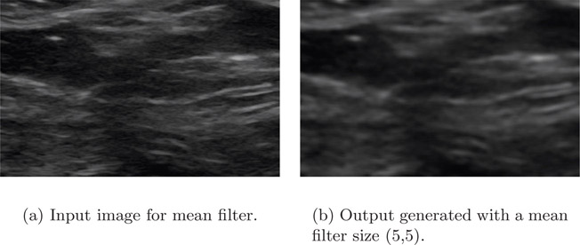
The program explaining the usage of the mean filter is given below. The filter (k) is an ndarray array of size 5-by-5 with all values = 1/25. The filter is then convolved using the “convolve” function from scipy.ndimage.filters.
import cv2import numpy as npimport scipy.ndimage# Opening the image using cv2.a = cv2.imread('../Figures/ultrasound_muscle.png')# Converting the image to grayscale.a = cv2.cvtColor(a, cv2.COLOR_BGR2GRAY)# Initializing the filter of size 5 by 5.# The filter is divided by 25 for normalization.k = np.ones((5,5))/25# performing convolutionb = scipy.ndimage.filters.convolve(a, k)# Writing b to a file.cv2.imwrite('../Figures/mean_output.png', b)
Figure 4.2(a) is an ultrasound image of muscle. Notice that the image contains noise. The mean filter of size 5-by-5 is applied to remove the noise. The output is shown in Figure 4.2(b). The mean filter effectively removed the noise but in the process blurred the image.
Advantages of the mean filter
•Removes noise.
•Enhances the overall quality of the image, i.e., mean filter brightens an image.
Disadvantages of the mean filter
•In the process of smoothing, the edges get blurred.
•Reduces the spatial resolution of the image.
If the coefficients of the mean filter are not all 1s, then the filter is a weighted mean filter. In the weighted mean filter, the filter coefficients are multiplied with the sub-image as in the non-weighted filter. After application of the filter, the image should be divided by the total weight for normalization.
Functions that do not satisfy Equation 4.2 are non-linear. The median filter is one of the most popular non-linear filters. A sliding window is chosen and is placed on the image at the pixel position (i, j). All pixel values under the filter are collected. The median of these values is computed and is assigned to (i, j) in the filtered image. For example, consider a 3-by-3 sub-image with values 5, 7, 6, 10, 13, 15, 14, 19, 23. To compute the median, the values are arranged in ascending order, so the new list is: 5, 6, 7, 10, 13, 14, 15, 19, and 23. Median is a value that divides the list into two equal halves; in this case it is 13. So the pixel (i, j) will be assigned 13 in the filtered image. The median filter is most commonly used in removing salt-and-pepper noise and impulse noise. Salt-and-pepper noise is characterized by black and white spots randomly distributed in an image.
The following is the Python function for the median filter:
scipy.ndimage.filters.median_filter(input, size=None,footprint=None, mode='reflect', cval=0.0, origin=0)Necessary arguments:input is the input image as an ndarray.Optional arguments:size can be a scalar or a tuple. For example, if theimage is 2D, size = 5 implies a 5-by-5 filter isconsidered. Alternately, the size can also be specifiedas size=(5,5).footprint is a boolean array of the same dimension asthe size unless specified otherwise. The pixels in theinput image corresponding to the points to thefootprint with true values are considered forfiltering.mode determines the method for handling the arrayborder by padding. Options are: constant,reflect, nearest, mirror, wrap.Returns: output image as an ndarray.
The Python code for the median filter is given below:
import cv2import scipy.ndimage# Opening the image and converting it to grayscale.a = cv2.imread('../Figures/ct_saltandpepper.png')# Converting the image to grayscale.a = cv2.cvtColor(a, cv2.COLOR_BGR2GRAY)# Performing the median filter.b = scipy.ndimage.filters.median_filter(a, size=5)# Saving b as median_output.png in Figures foldercv2.imwrite('../Figures/median_output.png', b)
In the above code, size = 5 represents a filter (mask) of size 5-by-5. The image in Figure 4.3(a) is a CT slice of the abdomen with salt-and-pepper noise. The image is read using ‘cv2.imread’ and the ndarray returned is passed to the median_filter function. The output of the median_filter function is stored as a ‘png’ file. The output image is shown in Figure 4.3(b). The median filter efficiently removed the salt-and-pepper noise.

This filter enhances the bright points in an image. In this filter the maximum value in the sub-image replaces the value at (i, j). The Python function for the maximum filter has the same arguments as the median filter discussed above. The Python code for the max filter is given below.
import scipy.miscimport scipy.ndimagefrom scipy.misc.pilutil import Image# opening the image and converting it to grayscalea = Image.open('../Figures/wave.png').convert('L')# performing maximum filterb = scipy.ndimage.filters.maximum_filter(a, size=5)# b is converted from an ndarray to an imageb = scipy.misc.toimage(b)b.save('../Figures/maxo.png')
The image in Figure 4.4(a) is the input image for the max filter. The input image has a thin black boundary on the left, right and bottom. After application of the max filter, the white pixels have grown and hence the thin edges in the input image are replaced by white pixels in the output image as shown in Figure 4.4(b).

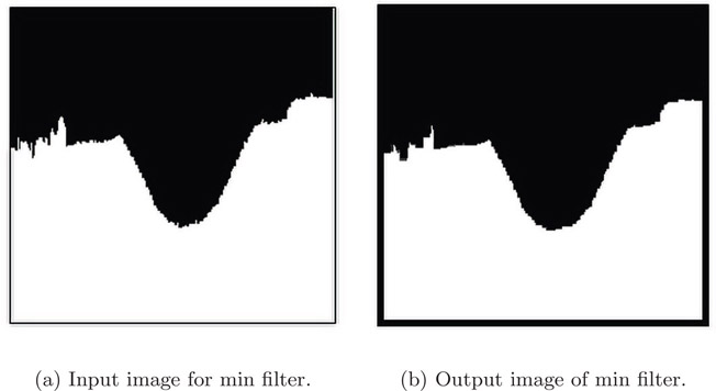
This filter is used to enhance the darkest points in an image. In this filter, the minimum value of the sub-image replaces the value at (i, j). The Python function for the minimum filter has the same arguments as the median filter discussed above. The Python code for the min filter is given below.
import cv2import scipy.ndimage# opening the image and converting it to grayscalea = cv2.imread('../Figures/wave.png')# performing minimum filterb = scipy.ndimage.filters.minimum_filter(a, size=5)# saving b as mino.pngcv2.imwrite('../Figures/mino.png', b)
After application of the min filter to the input image in Figure 4.5(a), the black pixels have grown and hence the thin edges in the input image are thicker in the output image as shown in Figure 4.5(b).
4.3Edge Detection using Derivatives
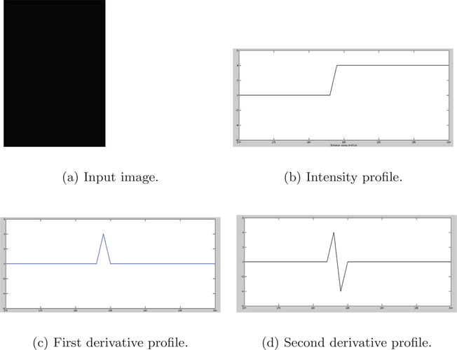
Edges are a set of points in an image where there is a change of intensity between one side of that point and the other. From calculus, we know that the changes in intensity can be measured by using the first or second derivative. First, let us learn how changes in intensities affect the first and second derivatives by considering a simple image and its corresponding profile. This method will form the basis for using first and second derivative filters for edge detection. Interested readers can also refer to [MH80],[Mar72],[PK91] and [Rob77].
Figure 4.6(a) is the input image in grayscale. The left side of the image is dark while the right side is light. While traversing from left to right, at the junction between the two regions, the pixel intensity changes from dark to light. Figure 4.6(b) is the intensity profile across a horizontal cross-section of the input image. Notice that at the point of transition from dark region to light region, there is a change in intensity in the profile. Otherwise, the intensity is constant in the dark and light regions. For clarity, only the region around the point of transition is shown in the intensity profile (Figure 4.6(b)), first derivative (Figure 4.6(c)), and second derivative (Figure 4.6(d)) profiles. In the transition region, since the intensity profile is increasing, the first derivative is positive, while being zero in the dark and light regions. The first derivative has a maximum or peak at the edge. Since the first derivative is increasing before the edge, the second derivative is positive before the edge. Likewise, since the first derivative is decreasing after the edge, the second derivative is negative after the edge. Also, the second derivative is zero in dark and light regions as the corresponding first derivative is zero. At the edge, the second derivative is zero. This phenomenon of the second derivative changing the sign from positive before the edge to negative after the edge or vice versa is known as zero-crossing, as it takes a value of zero at the edge. The input image was simulated on a computer and does not have any noise. However, acquired images will have noise that may affect the detection of zero-crossing. Also, if the intensity changes rapidly in the profile, spurious edges will be detected by the zero-crossing. To prevent the issues due to noise or rapidly changing intensity, the image is pre-processed before application of a second derivative filter.
An image is not a continuous function and hence derivatives are calculated using discrete approximations and not using functions. For the purpose of learning, let us look at the definition of the gradient of a continuous function and then extend it to discrete cases. If f(x, y) is a continuous function, then the gradient of f as a vector is given by
(4.3) |
|---|
where is known as the partial derivative of f with respect to x, (change of f along the horizontal direction) and is known as the partial derivative of f with respect to y, (change of f along the vertical direction). For more details refer to [Sch04]. The magnitude of the gradient is a scalar quantity and is given by
(4.4) |
|---|
where |z| is the norm of z.
For computational purposes, we will use the simplified version of the gradient given by Equation 4.5 and the angle given by Equation 4.6.
(4.5) |
|---|
(4.6) |
|---|
One of the most popular first derivative filters is the Sobel filter. The Sobel filter or mask is used to find horizontal and vertical edges as given in Table 4.3.
TABLE 4.3: Sobel masks for horizontal and vertical edges.

To understand how filtering is performed, let us consider a sub-image of size 3-by-3 given in Table 4.4 and multiply the sub-image with horizontal and vertical Sobel masks. The corresponding output is given in Table 4.5.
TABLE 4.4: A 3-by-3 subimage.
|
f1 |
f2 |
f3 |
|
f4 |
f5 |
f6 |
|
f7 |
f8 |
f9 |
TABLE 4.5: Output after multiplying the sub-image with Sobel masks.
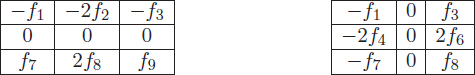
Since fx is the partial derivative of f in the x direction, which is a change of f along the horizontal direction, the partial derivative can be obtained by taking the difference between the third row and the first row in the horizontal mask, so fx = (f7 + 2f8 + f9) + ( − f1 − 2f2 − f3). Likewise, fy is the partial derivative of f in the y direction, which is a change of f in the vertical direction; the partial derivative can be obtained by taking the difference between the third column and the first column in the vertical mask, so fy = (f3 + 2f6 + f9) + ( − f1 − 2f4 − f7).
Using fx and fy f5, the discrete gradient at f5 (Equation 4.7) can be calculated.
(4.7) |
|---|
The important features of the Sobel filter are:
•The sum of the coefficients in the mask image is 0. This means that the pixels with constant grayscale are not affected by the derivative filter.
•The side effect of derivative filters is creation of additional noise. Hence, coefficients of +2 and −2 are used in the mask image to produce smoothing.
The following is the Python function for the Sobel filter:
scipy.ndimage.sobel(image)Necessary arguments:image is an ndarray with one or three channels.Returns: output is an ndarrray.
The Python code for the Sobel filter is given below.
import cv2from scipy import ndimage# Opening the image.a = cv2.imread('../Figures/cir.png')# Converting a to grayscale .a = cv2.cvtColor(a, cv2.COLOR_BGR2GRAY)# Performing Sobel filter.b = ndimage.sobel(a)# Saving b.cv2.imwrite('../Figures/sobel_cir.png', b)
As can be seen in the code, the image, ’cir.png’ is read using cv2.imread. The ndarray ‘a’ is then passed to the scipy.ndimage.sobel function to produce the Sobel edge enhanced image which is then written to file.
Another popular first derivative filter is Prewitt [Pre70]. The masks for the Prewitt filter are given in Table 4.6.
TABLE 4.6: Prewitt masks for horizontal and vertical edges.

As in the case of the Sobel filter, the sum of the coefficients in Prewitt is also 0. Hence this filter does not affect pixels with constant grayscale. However, the filter does not reduce noise like the Sobel filter.
For Prewitt, the Python function’s argument is similar to the Sobel function’s argument.
Let us consider an example to illustrate the effect of filtering an image using both Sobel and Prewitt. The image in Figure 4.7(a) is a CT slice of a human skull near the nasal area. The output of the Sobel and Prewitt filters is given in Figures 4.7(b) and 4.7(c). Both filters have successfully created the edge image.

Slightly modified Sobel and Prewitt filters can be used to detect one or more types of edges. Sobel and Prewitt filters to detect diagonal edges are given in Tables 4.7 and 4.8.
TABLE 4.7: Sobel masks for diagonal edges.

TABLE 4.8: Prewitt masks for diagonal edges.

To detect vertical and horizontal edges for Sobel and Prewitt filters we will use filters from the module skimage.
•The function filters.sobel_v computes vertical edges using the Sobel filter.
•The function filters.sobel_h computes horizontal edges using the Sobel filter.
•The function filters.prewitt_v computes vertical edges using the Prewitt filter.
•The function filters.prewitt_h computes horizontal edges using the Prewitt filter.
For example, for vertical edge detection, use prewitt_v and the Python function definition is:
from skimage import filters# The input to filter.prewitt_v has to be a numpy array.filters.prewitt_v(image)
Figure 4.8 is an example of detection of horizontal and vertical edges using the Sobel and Prewitt filters. The vertical Sobel and Prewitt filters have enhanced all the vertical edges, while the corresponding horizontal filters enhanced the horizontal edges and the regular Sobel and Prewitt filters enhanced all edges.

Another popular filter for edge detection is the Canny filter or Canny edge detector [Can86]. This filter uses three parameters to detect edges. The first parameter is the standard deviation, σ, for the Gaussian filter. The second and third parameters are the threshold values, t1 and t2. The Canny filter can be best described by the following steps:
1.A Gaussian filter is used on the image for smoothing.
2.An important property of an edge pixel is that it will have a maximum gradient magnitude in the direction of the gradient. So, for each pixel, the magnitude of the gradient given in Equation 4.5 and the corresponding direction, are computed.
3.At the edge points, the first derivative will have either a minimum or a maximum. This implies that the magnitude (absolute value) of the gradient of the image at the edge points is maximum. We will refer to these points as ridge pixels. To identify edge points and suppress others, only ridge tops are retained and other pixels are assigned a value of zero. This process is known as non-maximal suppression.
4.Two thresholds, low threshold and high threshold, are then used to threshold the ridges. Ridge pixel values help to classify edge pixels into weak and strong. Ridge pixels with values greater than the high threshold are classified as strong edge pixels, whereas the ridge pixels between low threshold and high threshold are called weak edge pixels.
5.In the last step, the weak edge pixels are 8-connected with strong edge pixels.
The Python function that is used for the Canny filter is:
cv2.Canny(image)Necessary arguments:input is the input image as an ndarrayReturns: output is an ndarray.
The Python code for the Canny filter is given below. The code does not need much explanation.
import cv2# Opening the image.a = cv2.imread('../Figures/maps1.png')# Performing Canny edge filter.b = cv2.Canny(a, 100, 200)# Saving b.cv2.imwrite('../Figures/canny_output.png', b)
Figure 4.9(a) is a simulated map consisting of names of geographical features of Antarctica. The Canny edge filter is used on this input image to obtain only edges of the letters as shown in Figure 4.9(b). Note that the edge of the characters are clearly marked in the output.

4.3.2Second Derivative Filters
As the name indicates, in the second derivative filter, the second derivative is computed in order to determine the edges. Since it requires computing the derivative of a derivative image, it is computationally expensive compared to the first derivative filter.
One of the most popular second derivative filters is the Laplacian. The Laplacian of a continuous function is given by:
where is the second partial derivative of f in the x direction represents a change of along the horizontal direction and is the second partial derivative of f in the y direction represents a change of along the vertical direction. For more details, refer to [Eva10] and [GT01]. The discrete Laplacian used for image processing has several versions. Most widely used Laplacian masks are given in Table 4.9.
TABLE 4.9: Laplacian masks.

The Python function that is used for the Laplacian along with the arguments is the following:
scipy.ndimage.filters.laplace(input, output=None,mode='reflect', cval=0.0)Necessary arguments:input is the input image as an ndarrayOptional arguments:mode determines the method for handling the arrayborder by padding. Different options are: constant,reflect, nearest, mirror, wrap.cval is a scalar value specified when the option formode is constant. The default value is 0.0.origin is a scalar that determines origin of thefilter. The default value 0 corresponds to a filterwhose origin (reference pixel) is at the center. In a2D case, origin = 0 would mean (0,0).Returns: output is an ndarray
The Python code for the Laplacian filter is given below. The Laplacian is called using the scipy laplace function along with the optional mode for handling array borders.
import cv2import scipy.ndimage# Opening the image.a = cv2.imread('../Figures/imagefor_laplacian.png')# Performing Laplacian filter.b = scipy.ndimage.filters.laplace(a,mode='reflect')cv2.imwrite('../Figures/laplacian_new.png',b)
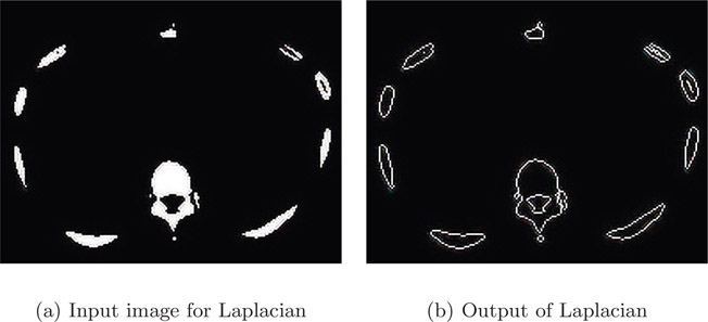
The black-and-white image in Figure 4.10(a) is a segmented CT slice of a human body across the rib cage. The various blobs in the image are the ribs. The Laplacian filter obtained the edges without any artifact.
As discussed earlier, a derivative filter adds noise to an image. The effect is magnified when the first derivative image is differentiated again (to obtain a second derivative) as in the case of second derivative filters. Figure 4.11 displays this effect. The image in Figure 4.11(a) is an MRI image from a brain scan. As there are several edges in the input image, the Laplacian filter over-segments the object (creates many edges) as seen in the output, Figure 4.11(b). This results in a noisy image with no discernible edges.

4.3.2.2Laplacian of Gaussian Filter
To offset the noise effect from the Laplacian, a smoothing function, Gaussian, is used along with the Laplacian. While the Laplacian calculates the zero-crossing and determines the edges, the Gaussian smooths the noise induced by the second derivative.
The Gaussian function is given by
(4.8) |
|---|
where r2 = x2 + y2 and σ is the standard deviation. A convolution of an image with the Gaussian will result in smoothing of the image. The σ determines the magnitude of smoothing. If σ is large then there will be more smoothing, which causes sharp edges to be blurred. Smaller values of σ produce less smoothing.
The Laplacian convolved with Gaussian is known as the Laplacian of Gaussian and is denoted by LoG. Since the Laplacian is the second derivative, the LoG expression can be obtained by finding the second derivative of G with respect to r, which yields
(4.9) |
|---|
The LoG mask or filter of size 5-by-5 is given in Table 4.10.
TABLE 4.10: Laplacian of Gaussian mask
|
0 |
0 |
−1 |
0 |
0 |
|
0 |
−1 |
−2 |
−1 |
0 |
|
−1 |
−2 |
16 |
−2 |
−1 |
|
0 |
−1 |
−2 |
−1 |
0 |
|
0 |
0 |
−1 |
0 |
0 |
The following is the Python function for LoG:
scipy.ndimage.filters.gaussian_laplace(input,sigma, output=None, mode='reflect', cval=0.0)Necessary arguments:input is the input image as an ndarray.sigma a floating point value is the standard deviationof the Gaussian.Returns: output is an ndarray
The Python code below shows the implementation of the LoG filter. The filter is invoked using the gaussian_laplace function with a sigma of 1.
import cv2import scipy.ndimage# Opening the image.a = cv2.imread('../Figures/vhuman_t1.png')# Performing Laplacian of Gaussian.b = scipy.ndimage.filters.gaussian_laplace(a, sigma=1,mode='reflect')cv2.imwrite('../Figures/log_vh1.png', b)
Figure 4.12(a) is the input image and Figure 4.12(b) is the output after the application of LoG. The LoG filter was able to determine the edges more accurately compared to the Laplacian alone (Figure 4.11(b)). However, the non-uniform foreground intensity has contributed to formation of blobs (a group of connected pixels).
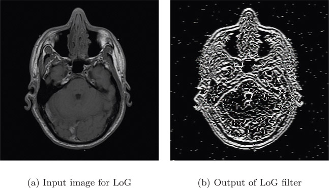
The major disadvantage of LoG is the computational price as two operations, Gaussian followed by Laplacian, have to be performed. Even though LoG segments the object from the background, it over-segments the edges within the object causing closed loops (also called the spaghetti effect) as shown in the output Figure 4.12(b).
The Frangi filter [AFFV98] is used to detect vessel-like objects in an image. We will begin the discussion with the fundamental idea of the Frangi filter before discussing the math behind it. Figure 4.4.1 contains two objects. One of the objects is elongated in one direction but not the other, while the second object is almost square. The orthogonal arrows are drawn to be proportional to the length along a given direction. This qualitative geometrical difference can be quantified by finding the eigen values for these two objects. For the elongated object, the eigen value will be larger in the direction of the longer arrow and smaller along the direction of the smaller arrow. On the other hand, for the square object, the eigen value along the direction of the longer arrow is similar to the eigen value along the direction of the smaller arrow. The Frangi filter computes the eigen value on the second derivative (Hessian) image instead of computing the eigen value on the original image.

To reduce noise due to derivatives, the image is smoothed by convolution. Generally, Gaussian smoothing is used. It can be shown that finding the derivative of Gaussian smoothed convolved image is equivalent to finding derivative of a Gaussian convolved with an image. We will determine the second derivative of Gaussian using the formula below where gσ is a Gaussian.
(4.10) |
|---|
We will then determine the local second derivative (Hessian) and its eigen value. For a 2D image, there will be two eigen values (λ1 and λ2) for each pixel coordinate. The eigen values are then sorted in increasing order. A pixel is considered to be part of a tubular or vessel-like structure if λ1 ≈ 0 while |λ2| > |λ1|.
For a 3D image, there will be three eigen values (λ1, λ2 and λ3) for each voxel coordinate. The eigen values are then sorted in increasing order. A voxel is considered to be part of a tubular or vessel-like structure if λ1 ≈ 0 while λ2 and λ3 are approximately the same high absolute value and are of the same sign. The bright vessels will have positive values for λ2 and λ3 while darker vessels will have negative values for λ2 and λ3.
In the code below, we will demonstrate using the Frangi filter programmatically. The image is first opened and converted to grayscale. The image is converted to a numpy array using the np.array function so that it can be fed to the Frangi filter. Finally, a call is made to the Frangi filter located in the skimage.filters module. The output of the frangi function is then saved to a file.
import cv2import numpy as npimport numpy as npfrom PIL import Imagefrom skimage.filters import frangiimg = cv2.imread('../Figures/angiogram1.png')img1 = np.asarray(img)img2 = frangi(img1, black_ridges=True)img3 = 255*(img2-np.min(img2))/(np.max(img2)-np.min(img2))cv2.imwrite('../Figures/frangi_output.png', img3)
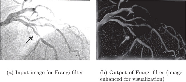
The image in Figure 4.14(a) is the input to the Frangi filter and the image in Figure 4.14(b) is the output of the Frangi filter. The input image is an angiogram that clearly shows multiple vessels enhanced by contrast. The output image contains only pixels that are in the vessel. The contrast of the output image was enhanced for the sake of publication.
•The mean filter smooths the image while blurring the edges in the image.
•The median filter is effective in removing salt-and-pepper noise.
•The most widely used first derivative filters are Sobel, Prewitt and Canny.
•Both Laplacian and LoG are popular second derivative filters. The Laplacian is very sensitive to noise. In LoG, the Gaussian smooths the image so that the noise from the Laplacian can be compensated. But LoG suffers from the spaghetti effect.
•The Frangi filter is used for detecting vessel-like structures.
1.Write a Python program to apply a mean filter on an image with salt-and-pepper noise. Describe the output, including the mean filter’s ability to remove the noise.
2.Describe how effective the mean filter is in removing salt-and-pepper noise. Based on your understanding of the median filter, can you explain why the mean filter cannot remove salt-and-pepper noise?
3.Can max filter or min filter be used for removing salt-and-pepper noise?
4.Check the scipy documentation available at http://docs.scipy.org/doc/scipy/reference/ndimage.html. Identify the Python function that can be used for creating custom filters.
5.Write a Python program to obtain the difference of the Laplacian of Gaussian (LoG). The pseudo code for the program will be as follows:
(a)Read the image.
(b)Apply the LoG filter assuming a standard deviation of 0.1 and store the image as im1.
(c)Apply the LoG filter assuming a standard deviation of 0.2 and store the image as im2.
(d)Find the difference between the two images and store the resulting image?
6.In this chapter, we have discussed a few spatial filters. Identify two more filters and discuss their properties.