The modern light microscope was created in the 17th century, but the origin of its important component, the lens, dates back more than three thousand years. The ancient Greeks used lenses as burning glasses, by focusing the sun’s rays. In later years, lenses were used to create glasses in Europe in order to correct vision problems. The scientific use of lenses can be dated back to the 16th century with the creation of compound microscopes. Robert Hooke, an English physicist, was the first person to describe cells using a microscope. Antonie van Leeuwenhoek, a Dutch physicist, improved on the lens design and made many important discoveries. For all his research efforts, he is referred to as “the father of microscopy.”
We begin this chapter with an introduction to the various physical principles that govern image formation in light microscopy. These include geometric optics, diffraction limit of the resolution, the objective lens, and the numerical aperture. The aim of a microscope is to magnify an object while maintaining good resolving power (i.e., the ability to distinguish two objects that are nearby). The diffraction limit, the objective lens, and the numerical aperture determine the resolving power of a microscope. We apply these principles during the discussion on design of a simple wide-field microscope. This is followed by the fluorescence microscope that not only images the structure but also encodes the functions of the various parts of the specimen. We then discuss confocal and Nipkow disk microscopes that offer better contrast resolution compared to wide-field microscopes. We conclude with a discussion on choosing a wide-field or confocal microscope for a given imaging task. Interested readers can refer to [Bir11], [Dim12],[HL93],[Mer10],[RDLF05],[Spl10] for more details.
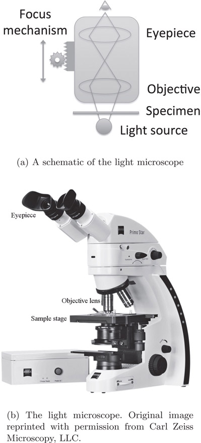
A simple light microscope of today is shown in Figure 15.1. It consists of an eyepiece, an objective lens, the specimen to be viewed and a light source. As the name indicates, the eyepiece is the lens for viewing the sample. The objective is the lens closest to the sample. The eyepiece and the objective lens are typically compound convex lenses. With the introduction of digital technology, the viewer does not necessarily look at the sample through the eyepiece but instead a camera acquires and stores the image.
The lenses used in a microscope have magnification that allows objects to appear larger than their original size. Thus, the magnification for the objective can be defined as the ratio of the height of the image formed to the height of the object. Applying triangular inequality (Figure 15.2), we can also obtain the magnification, m, as the ratio of d1 to d0.
(15.1) |
|---|

A similar magnification factor can be obtained for the eyepiece as well. The total magnification of the microscope can be obtained as the product of the two magnifications.
(15.2) |
|---|
Numerical aperture defines both the resolution and the photon-collecting capacity of a lens. It is defined as:
(15.3) |
|---|
where θ is the angular aperture or the acceptance angle of the aperture and n is the refractive index.
For high-resolution imaging, it is critical (as will be discussed later) to use an objective with a high numerical aperture. Figure 15.3 is a photograph of an objective with all the parameters embossed. In this example, 20X is the magnification and 0.40 is the numerical aperture.
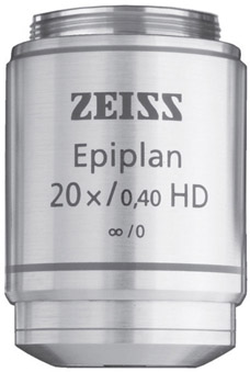
FIGURE 15.3: Markings on the objective lens. Original image reprinted with permission from Carl Zeiss Microscopy, LLC.
Resolution is an important characteristic of an imaging system. It defines the smallest detail that can be resolved (or viewed) using an optical system like the microscope. The limiting resolution is called the diffraction limit. We know that electromagnetic radiations have both particle and wave natures. The diffraction limit is due to the wave nature. The Huygens-Fresnel principle suggests that an aperture such as a lens creates secondary wave sources from an incident plane wave. These secondary sources create an interference pattern and produce the Airy disk.
Based on the diffraction principles, we can derive the resolving power of a lens. It is the minimum distance between two adjacent points that can be distinguished through a lens. It is defined as:
(15.4) |
|---|
If a microscope system consists of both objective and eyepiece, then the formula has to be modified to:
(15.5) |
|---|
where NAobj and NAeye are the numerical apertures of the objective and eyepiece respectively.
The aim of any optical imaging system is to improve the resolving power or reduce the value of RP. This can be achieved by decreasing the wavelength, increasing the aperture angle, or increasing the refractive index. Since this discussion is on the optical microscope, we are limited to the visible wavelength of light. X-rays, gamma rays, etc., have shorter wavelengths compared to visible light and hence better resolving power. The refractive index (discussed later) of air is 1.00. The refractive index of mediums used in microscopy imaging is generally greater than 1.00 and hence improves resolving power.
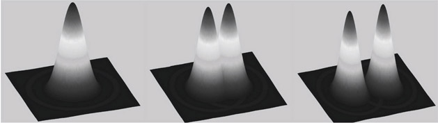
Two points separated by large distances will have distinct Airy disks and hence can be easily identified by an observer. If the points are close (middle image in Figure 15.4), the two Airy disks begin to overlap. If the distance between points is further reduced (left image in Figure 15.4), they begin to further overlap. The two peaks approach and the limit at which the human eye cannot separate the two points is referred to as the Rayleigh Criterion.
In the setup shown in Figure 15.1, the two sources of magnification are the objective lens and eyepiece. Since the objective is the closest to the specimen, it is the largest contributor of magnification. Thus, it is critical to understand the inner workings of the objective lens and also the various choices.
We begin the discussion with the refractive index. It is a dimensionless number that describes how electromagnetic radiation passes through various mediums. The refractive index can be seen in various phenomena such as rainbows, separation of visible light by prisms, etc. The refractive index of the lens is different from that of the specimen. This difference in refractive index causes the deflection of light. The refractive index between the objective lens and the specimen can be matched by submerging the specimen in a fluid (generally called medium) with the refractive index close to the lens.
Table 15.1 shows commonly used media and their refractive indexes. Failure to match the refractive index will result in loss of signal, contrast and resolving power.
Table 15.1 List of the commonly used media and their refractive indexes.
|
Medium |
Refractive Index |
|
Air |
1.0 |
|
Water |
1.3 |
|
Glycerol |
1.44 |
|
Immersion oil |
1.52 |
To summarize, the objective lens selection is based on the following parameters:
1.refractive index of the medium,
2.magnification needed,
3.resolution, which in turn is determined by the choice of numerical aperture.
15.2.5Point Spread Function (PSF)
In Chapter 4, we discussed that Gaussian smoothing is used to reduce noise in an image. The noise reduction is achieved by smearing the pixel value at one location to all its neighbors. Any optical system performs a similar operation with a kernel called a Point Spread Function (PSF). It is the response of an optical system to a point input or point object as a consequence of diffraction. When a point source of light is passed through a pinhole aperture, the resultant image on a focal plane is not a point, but instead the intensity is spread to multiple neighboring pixels. In other words, the point image is blurred by the PSF. The PSF is dependent on the numerical aperture of the lens. A lens with a high numerical aperture produces a PSF of smaller width.
Light microscopes can be classified into different types depending on the method used to acquire images, improve contrast, illuminate samples etc. The microscope that we have described is called a wide-field microscope. It suffers from poor spatial resolution (without any computer processing), and poor contrast resolution due to the effect of PSF.
15.3Construction of a Wide-Field Microscope
A light microscope (Figure 15.1) is designed to magnify the image of a sample using multiple lenses. It consists of the following:
1.Eyepiece
2.Objective
3.Light source
4.Condenser lens
5.Specimen stage
6.Focus knobs
The eyepiece is the lens closest to the eye. Modern versions of the eyepiece are compound lenses in order to compensate for aberrations. It is interchangeable and can be replaced by eyepieces of different magnification depending on the nature of object being imaged.
The objective is the lens closest to the object. These are generally compound lenses in order to compensate for aberrations. They are characterized by three parameters: magnification, numerical aperture and the refractive index of the immersion medium. The objectives are interchangeable and hence modern microscopes also contain a turret that contains multiple objectives to enable easier and faster switching between different lenses. The objective might be immersed in oil to match the refractive index and increase the numerical aperture and consequently increase the resolving power.
The light source is at the bottom of the microscope. It can be tuned to adjust the brightness in the image. If the lighting is poor, the contrast of the resultant image will be poor, while excess light might saturate the camera recording the image. The most commonly used illumination method is Köhler illumination, designed by August Köhler in 1893. The previous methods suffered from non-uniform illumination, projection of the light source on the imaging plane, etc. Köhler illumination eliminates non-uniform illumination so that all parts of the light source contribute to specimen illumination. It works by ensuring that the lamp image is not projected on the sample plane with the use of a collector lens placed near the lamp. This lens focuses the image of the lamp to the condenser lens. Under this condition, illumination of the specimen is uniform.
The specimen stage is used for placing the specimen under examination. The stage can be adjusted to move along its two axes, so that a large specimen can be imaged. Depending on the features of a microscope, the stage could be manual or motor controlled.
Focus knobs allow moving the stage or objective in the vertical axis. This allows focusing of the specimen and also enables imaging of large objects.
In the microscope setup shown in Figure 15.1, the specimen is illuminated by using a light source placed below. This is called trans-illumination. This method does not separate the emission and excitation light in fluorescence microscopy. An alternate method called epi-illumination is used in modern microscopes.
In this method (Figure 15.7), the light source is placed above the specimen. The dichroic mirror reflects the excitation light and illuminates the specimen. The emitted light (which is of longer wavelength) travels through the dichroic mirror and is either viewed or detected using a camera. Since there are two clearly defined paths for emission and excitation light, only the emitted light is used in the formation of the image and hence improves the quality of the image.
A fluorescence microscope allows identification of various parts of the specimen not only in terms of structure but also in terms of function. It allows tagging different parts of the specimen, so that it generates light of certain wavelengths and forms an image. This improves the contrast in the image between various objects in a specimen.
Fluorescence is generally observed when a fluorescent molecule absorbs light at a particular wavelength and emits light at a different wavelength within a short interval. The molecule is generally referred to as fluorochrome or dye, and the delay between absorption and emission is in the order of nanoseconds. This process is generally shown diagrammatically using the Jablonski diagram shown in Figure 15.5. The figure should be read from bottom to top. The lower state is the stable ground state, generally called the S0 state. A light or photon incident on the fluorochrome causes the molecule to reach an excited state (S′1). A molecule in the excited state is not stable and hence returns to its stable state after losing the energy both in the form of radiation such as heat and also light of longer wavelength. This light is referred to as the emitted light.

From Planck’s law that was discussed in Chapter 13, the energy of light is inversely proportional to the wavelength. Thus, light of higher energy will have shorter wavelength and vice versa. The incident photon is a higher energy and hence shorter wavelength, while the emitted light is of low energy and longer wavelength. The exact mechanisms of emission and absorption are beyond the scope of this book and readers are advised to consult books dedicated to fluorescence for details.
15.5.2Properties of Fluorochromes
Two properties of fluorochromes, excitation wavelength and emission wavelength, were discussed in the previous section. Table 15.2 lists the excitation and emission wavelengths of commonly used fluorochromes. As can be seen in the table, the difference between excitation and emission wavelengths, or the Stokes shift, is significantly different for different dyes. The larger the difference, the easier it is to filter the signal between emission and excitation.
Table 15.2 List of the fluorophores of interest to fluorescence imaging.
|
Fluorochrome |
Peak Excitation Wavelength (nm) |
Peak Emission Wavelength (nm) |
Stokes Shift (nm) |
|
DAPI |
358 |
460 |
102 |
|
FITC |
490 |
520 |
30 |
|
Alexa Fluor 647 |
650 |
670 |
20 |
|
Lucifer Yellow VS |
430 |
536 |
106 |
A third property, quantum yield, is another important characteristic of a dye. It is defined as:
(15.6) |
|---|
Another important property that determines the amount of fluorescence generated is the absorption cross-section. The absorption cross-section can be explained with the following analogy. If a bullet is fired at a target, the ability to reach the target is better if the target is large and if the target surface is oriented in the direction perpendicular to the direction of the bullet path. Similarly, the term absorption cross-section defines the “effective” cross-section of the fluorophore and hence the ability of the excitation light to produce fluorescence.
It is measured by exciting a sample of fluorophore of certain thickness with excitation photons of a certain intensity and measuring the intensity of the emitted light. The relationship between the two intensities is given by Equation 15.7.
(15.7) |
|---|
where I0 is the excitation photon intensity, I is the emitted photon intensity, σ is the absorption cross-section of the fluorophore, D is the density, and δx is the thickness of the fluorophore.
During fluorescence imaging, it is necessary to block all light that is not emitted by the fluorochrome to ensure the best contrast in the image and consequently better detection and image processing. In addition, the specimen does not necessarily contain only one type of fluorochrome. Thus, to separate the image created by one fluorochrome from the other, a filter that allows only light of a certain wavelength corresponding to the different fluorochromes is needed.
The filters can be classified into three categories: lowpass, bandpass and highpass. We discussed these as digital filters in Chapter 7 while here we will discuss physical filters. The lowpass filter allows light of shorter wavelength and blocks longer wavelengths. The highpass filter allows light of longer wavelength and blocks shorter wavelengths. The bandpass filter allows light of a certain range of wavelengths. In addition, fluorescence microscopy uses a special type of filter called a dichroic mirror (Figure 15.7). Unlike the three filters discussed earlier, in a dichroic mirror the incident light is at 45 ° to the filter. The mirror reflects light of shorter wavelength and allows longer wavelengths to pass through.
Multi-channel imaging is a mode where different types of fluorochromes are used for imaging resulting in images with multiple channels. Such images are called multi-channel images. Each channel contains an image corresponding to one fluorochrome. For example, if we obtained an image of size 512-by-512, using two different fluorochromes, the image would be of size 512-by-512-by-2. The two in the size corresponds to the two channels. Generally most fluorescence images have 3 dimensions. Hence the volume in such cases would be 512-by-512-by-200-by-2, where 200 is the number of slices or z-dimension. The actual number may vary based on the imaging conditions. The choice of the fluorochrome is dependent on the following parameters:
1.Excitation wavelength
2.Emission wavelength
3.Quantum yield
4.Photostability
Filters used in the microscope need to be chosen based on the fluorochrome being imaged.
Confocal microscopes overcome the issue of spatial resolution that affects wide-field microscopes. A better resolution in confocal microscopes is achieved by the following:
•A narrow beam of light illuminates a region of the specimen. This eliminates collection of light by the reflection or fluorescence due to a nearby region in the specimen.
•The emitted or reflected light arising from the specimen passes through a narrow aperture. A light emanating from the direction of the beam will pass through the aperture. Any light emanating from nearby objects or any scattered light from various objects in the specimen will not pass through the aperture. This process eliminates all out-of-focus light and collects only light in the focal plane.
The above process describes image formation at a single pixel. Since an image of the complete specimen needs to be formed, the narrow beam of light needs to be scanned all across the specimen and the emitted or reflected light needs to be collected to form a complete image. The scanning process is similar to the raster scanning process used in television. It can be operated using two methods. In the first method devised by Marvin Minsky, the specimen is translated so that all points can be scanned. This method is slow and also changes the shape of the specimen suspended in liquids and is no longer used. The second approach is to keep the specimen stationary while the light beam is scanned across the specimen. This was made possible by advances in optics and computer hardware and software, and is used in all modern microscopes.
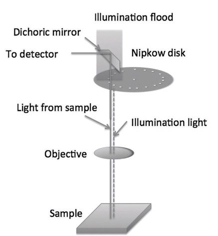
Paul Nipkow created and patented a method for converting an image into an electrical signal in 1884. The method consisted of scanning an image by using a spinning wheel containing holes placed in a spiral pattern, as shown in Figure 15.6. The portion of the wheel that does not contain the hole is darkened so that light does not pass through it. By rotating the disk at constant speed, a light passing through the hole scans all points in the specimen. This approach was later adapted to microscopy. Figure 15.6 shows only one spiral with a smaller number of holes while a commercially available disc will have a large number of holes, to allow fast image acquisition.

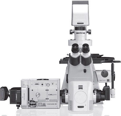
A setup containing the disk along with the laser source, objective lens, detector, and the specimen is shown in Figure 15.7, and Figure 15.8 is a photograph of a Nipkow disk microscope. In this figure, the illuminating light floods a significant portion of the holes. The portion that does not contain any holes reflects the light. The light that passes through the holes reaches the specimen through the objective lens. The reflected light, or the light emitted by fluorescence, passes through the objective and is reflected by the dichroic mirror. The detector forms an image using the reflected light.
Unlike a regular confocal microscope, the Nipkow disk microscope is faster as neither the specimen nor the light beam needs to be raster scanned. This enables rapid imaging of live cells.
Confocal and wide-field microscopes each have their own advantages and disadvantages. These factors need to be considered when making a decision on what microscope to use for a given cost or type of specimen or the analysis to be performed.
•Resolution: There are two different resolutions: xy and z directions. Confocal microscopes produce better resolution images in both directions. Due to advances in computing and better software, wide-field images can be deconvolved [WSS01] to a good resolution along x and y but not necessarily along the z direction.
•Photo bleaching: Images from a confocal microscope may be photo-bleached, as the specimen is imaged over a longer time period compared to a wide-field microscope.
•Noise: Wide-field microscopes generally produce images with less noise due to blurring from the PSF.
•Acquisition rate: Since confocal images scan individual points, it is generally slower compared to wide-field microscopes.
•Cost: As a wide-field microscope has fewer parts, it is less expensive than confocal.
•Computer processing: Confocal images need not be processed using deconvolution. Depending on the setup, deconvolution of a wide-field image can produce images of comparable quality to confocal images.
•Specimen composition: A wide-field microscope with deconvolution works well for a specimen with a small structure.
•The physical properties that govern optical microscope imaging are magnification, diffraction limits, and numerical aperture. The diffraction limit and numerical aperture determine the resolution of the image.
•The specimen is immersed in a medium in order to match the refractive index and to increase the resolution.
•Wide-field and confocal are the two most commonly used microscopes. In the former, a flood of light is used to illuminate the specimen while in the latter, a pencil beam is used to scan the specimen and the collected light passes through a confocal aperture.
•The fluorescence microscope allows imaging of the shape and function of the specimen. Fluorescence microscope images are obtained after the specimen has been treated with a fluorophore.
•The specific range of wavelength emitted by the fluorophore is measured by passing the light through a filter.
•To speed up confocal image acquisition, a Nipkow disk is used. The disk consists of a series of holes placed on a spiral. The disk is rotated and the position of the holes is designed to ensure that complete 2D scanning of the specimen is achievable.
1.If the objective has a magnification of 20X and the eyepiece has a magnification of 10X, what is the total magnification?
2.A turret has three objectives: 20X, 40X and 50X. The eyepiece has magnification of 10X. What is the highest magnification achievable?
3.In the same turret setup, if a cell occupies 10% of the field of view for an objective magnification of 20X, what would be the field of view percentage for 40X?
4.Discuss a few methods to increase spatial resolution in an optical microscope. What are the limits for each parameter?