5. Image Enhancement

Search in book...
Toggle Font Controls
Create new playlist

Name your new playlist

Playlist description (optional)
Sign In

Email address

Password

Forgot Password?

or

Continue with Facebook

Continue with Google
Sign Up

Full Name

Email address

Confirm Email Address

Password

or

Continue with Facebook

Continue with Google

In previous chapters we discussed image filters. The filter enhances the quality of an image so that important details can be visualized and quantified. In this chapter, we discuss a few more image enhancement techniques. These techniques transform the pixel values in the input image to a new value in the output image using a mapping function. We discuss logarithmic transformation, power law transformation, image inverse, histogram equalization, and contrast stretching. For more information on image enhancement refer to [HWJ98],[OR89],[PK81].

5.2Pixel Transformation

A transformation is a function that maps a set of inputs to a set of outputs so that each input has exactly one output. For example, T(x) = x² is a transformation that maps inputs to corresponding squares of input. Figure 5.1 illustrates the transformation T(x) = x² for three inputs.

FIGURE 5.1: Illustration of transformation T(x) = x².

In the case of images, a transformation takes the pixel intensities of the image as an input and creates a new image where the corresponding pixel intensities are defined by the transformation. Let us consider the transformation, T(x) = x + 50. When this transformation is applied to an image, a value of 50 is added to the intensity of each pixel. The corresponding image is brighter than the input image. Figures 5.2(a) and 5.2(b) are the input and output images of the transformation, T(x) = x + 50.

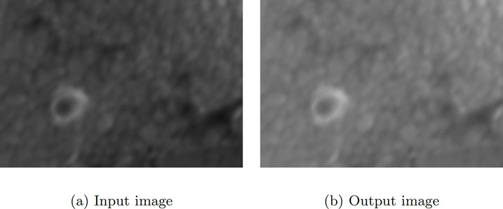
FIGURE 5.2: Example of transformation T(x) = x + 50. Original image reprinted with permission from Mr. Karthik Bharathwaj.

For a grayscale image, the transformation range is given by [0, L − 1] where L = 2^k and k is the number of bits in an image. In the case of an 8-bit image, the range is [0, 2⁸ − 1] = [0, 255] and for a 16-bit image the range is [0, 2¹⁶ − 1] = [0, 65535]. In this chapter we consider 8-bit grayscale images but the basic principles apply to images of any bit-depth.

5.3Image Inverse

Image inverse transformation is a linear transformation. The goal is to transform the dark intensities in the input image to bright intensities in the output image and vice versa. If the range of intensities is [0, L − 1] for the input image, then the image inverse transformation at (i, j) is given by the following

$t (i, j) = L - 1 - I (i, j)$ $t (i, j) = L - 1 - I (i, j)$	(5.1)

where I is the intensity value of the pixel in the input image at (i, j).

For an 8-bit image, the Python code for the image inverse is given below:

import cv2
 
 
# Opening the image.
im = cv2.imread(’../Figures/imageinverse_input.png’)
# Performing the inversion operation
im2 = 255 - im
# Saving the image as imageinverse_output.png in
# Figures folder.
cv2.imwrite(’../Figures/imageinverse_output.png’, im2)

Figure 5.3(a) is a CT image of the region around the heart. Notice that there are several metal objects, bright spots with streaks, emanating in the image. The bright circular object near the bottom edge is a rod placed in the spine, while two arch-shaped metal objects are the valves in the heart. The metal objects are very bright and prevent us from observing other details. The image inverse transformation suppresses the metal objects while enhancing other features of interest such as blood vessels, as shown in Figure 5.3(b).

FIGURE 5.3: Example of image inverse transformation. Original image reprinted with permission from Dr. Uma Valeti, Cardiovascular Imaging, University of Minnesota.

5.4Power Law Transformation

Power law transformation, also known as gamma-correction, is used to enhance the quality of the image. The power transformation at (i, j) is given by

$t (i, j) = k I (i, j)^{γ}$ $t (i, j) = k I (i, j)^{γ}$	(5.2)

where k and γ are positive constants and I is the intensity value of the pixel in the input image at (i, j). In most cases k = 1.

If γ = 1 (Figure 5.4), then the mapping is linear and the output image is the same as the input image. When γ < 1, a narrow range of dark or low-intensity pixel values in the input image get mapped to a wide range of intensities in the output image, while a wide range of bright or high intensity-pixel values in the input image get mapped to a narrow range of high intensities in the output image. The effect from values of γ > 1 is opposite that of values γ < 1. Considering that the intensity range is between [0, 1], Figure 5.4 illustrates the effect of different values of γ for k = 1.

FIGURE 5.4: Graph of power law transformation for different γ.

The human brain uses gamma-correction to process an image, hence gamma-correction is a built-in feature in devices that display, acquire, or publish images. Computer monitors and television screens have built-in gamma-correction so that the best image contrast is displayed in all the images.

In an 8-bit image, the intensity values range from [0, 255]. If the transformation is applied according to Equation 5.2, and for γ > 1 the output pixel intensities will be out of bounds. To avoid this scenario, in the following Python code the pixel intensities are normalized, $\frac{I (i, j)}{m a x (I)} = I_{n o r m} .$ $\frac{I (i, j)}{m a x (I)} = I_{n o r m} .$ For k = 1, replacing I(i, j) with I_norm and then applying the natural log, ln, on both sides of Equation 5.2 will result in

$\ln (t (i, j)) = \ln (I_{n o r m})^{γ} = γ * \ln (I_{n o r m}) .$ $\ln (t (i, j)) = \ln (I_{n o r m})^{γ} = γ * \ln (I_{n o r m}) .$	(5.3)

now, basing both sides by e will give us

$e^{\ln (t (i, j))} = e^{γ * \ln (I_{n o r m})} .$ $e^{\ln (t (i, j))} = e^{γ * \ln (I_{n o r m})} .$	(5.4)

Since e^ln(x) = x, the left side in the above equation will simplify to

$t (i, j) = e^{γ * \ln (I_{n o r m})} .$ $t (i, j) = e^{γ * \ln (I_{n o r m})} .$	(5.5)

To have the output in the range [0, 255] we multiply the right side of the above equation by 255 which results in

$t (i, j) = e^{γ * \ln (I_{n o r m})} * 255.$ $t (i, j) = e^{γ * \ln (I_{n o r m})} * 255.$	(5.6)

This transformation is used in the Python code for power law transformation given below.

import cv2
import matplotlib.pyplot as plt
import numpy as np
 
# Opening the image.
a = cv2.imread(’../Figures/angiogram1.png’)
# gamma is initialized.
gamma = 0.5
# b is converted to type float.
b1 = a.astype(float)
# Maximum value in b1 is determined.
b3 = np.max(b1)
# b1 is normalized
b2 = b1/b3
# gamma-correction exponent is computed.
b4 = np.log(b2)*gamma
# gamma-correction is performed.
c = np.exp(b4)*255.0
# c is converted to type int.
c1 = c.astype(int)
# Displaying c1
plt.imshow(c1)

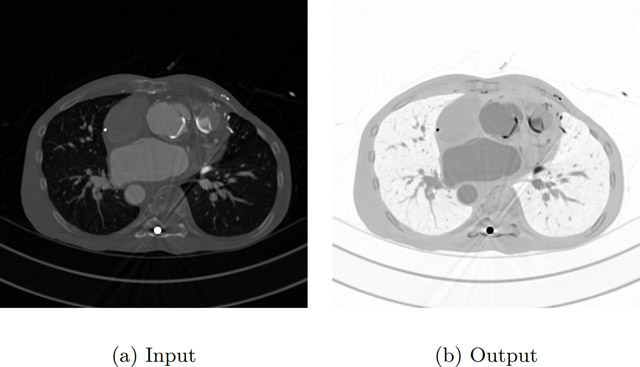
Figure 5.5(a) is an image of the angiogram of blood vessels. The image is too bright and it is quite difficult to distinguish the blood vessels from background. Figure 5.5(b) is the image after gamma correction with γ = 0.5; the image is brighter compared to the original image. Figure 5.5(c) is the image after gamma correction with γ = 5; this image is darker and the blood vessels are visible.

FIGURE 5.5: An example of power law transformation.

5.5Log Transformation

Log transformation is used to enhance pixel intensities that are otherwise missed due to a wide range of intensity values or lost at the expense of high-intensity values. If the intensities in the image range from [0, L − 1] then the log transformation at (i, j) is given by

$t (i, j) = k \log (1 + I (i, j))$ $t (i, j) = k \log (1 + I (i, j))$	(5.7)

where $k = \frac{L - 1}{\log (1 + | I_{m a x} |)}$ $k = \frac{L - 1}{\log (1 + | I_{m a x} |)}$ and I_max is the maximum magnitude value and I(i, j) is the intensity value of the pixel in the input image at (i, j). If both I(i, j) and I_max are equal to L − 1, then t(i, j) = L − 1. When I(i, j) = 0, since log (1) = 0 will give t(i, j) = 0. While the end points of the range get mapped to themselves, other input values will be transformed by the above equation. The log can be of any base; however, the common log (log base 10) or natural log (log base e) are widely used. The inverse of the above log transformation when the base is e is given by $t^{- 1} (x) = e^{\frac{x}{k}} - 1,$ $t^{- 1} (x) = e^{\frac{x}{k}} - 1,$ which does the opposite of the log transformation.

Similar to the power law transformation with γ < 1, the log transformation also maps a small range of dark or low-intensity pixel values in the input image to a wide range of intensities in the output image, while a wide range of bright or high-intensity pixel values in the input image get mapped to narrow range of high intensities in the output image. Considering the intensity range is between [0, 1], Figure 5.6 illustrates the log and inverse log transformations.

FIGURE 5.6: Graph of log and inverse log transformations.

The Python code for log transformation is given below.

import cv2
import numpy, math
 
 
# Opening the image.
a = cv2.imread(’../Figures/bse.png’)
# a is converted to type float.
b1 = a.astype(float)
# Maximum value in b1 is determined.
b2 = numpy.max(b1)
# Performing the log transformation.
c = (255.0*numpy.log(1+b1))/numpy.log(1+b2)
# c is converted to type int.
c1 = c.astype(int)
# Saving c1 as logtransform_output.png.
cv2.imwrite(’../Figures/logtransform_output.png’, c1)

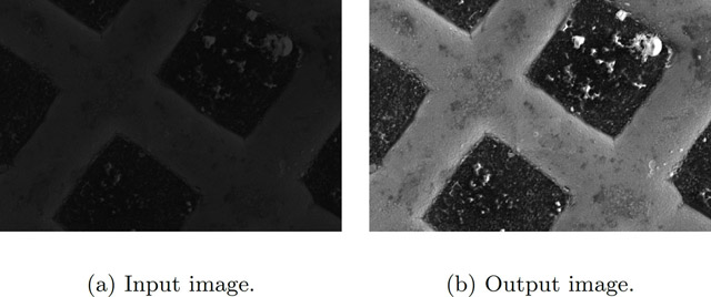
Figure 5.7(a) is a backscattered electron microscope image. Notice that the image is very dark and the details are not clearly visible. Log transformation is performed to improve the contrast, to obtain the output image shown in Figure 5.7(b).

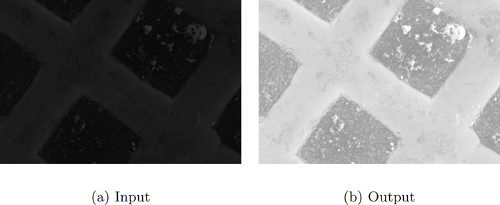
FIGURE 5.7: Example of log transformation. Original image reprinted with permission from Mr. Karthik Bharathwaj.

5.6Histogram Equalization

The histogram of an image was discussed in Chapter 3, “Image and its Properties.” The histogram of an image is a discrete function, its input is the gray-level value and the output is the number of pixels with that gray-level value and can be given as h(x_n) = y_n. In a grayscale image, the intensities of the image take values between [0, L − 1]. As discussed earlier, low gray-level values in the image (the left side of the histogram) correspond to dark regions and high gray-level values in the image (the right side of the histogram) correspond to bright regions.

In a low-contrast image, the histogram is narrow, whereas in an image with better contrast, the histogram is spread out. In histogram equalization, the goal is to improve the contrast of an image by rescaling the histogram so that the histogram of the new image is spread out and the pixel intensities range over all possible gray-level values. The rescaling of the histogram will be performed by using a transformation. To ensure that for every gray-level value in the input image there is a corresponding output, a one-to-one transformation is required; that is, every input has a unique output. This means the transformation should be a monotonic function. This will ensure that the transformation is invertible.

Before histogram equalization transformation is defined, the following should be computed:

•The histogram of the input image is normalized so that the range of the normalized histogram is [0, 1].

•Since the image is discrete, the probability of a gray-level value, denoted by p_x(i), is the ratio of the number of pixels with a gray value i to the total number of pixels in the image. This is generally called the probability distribution function (PDF).

•The cumulative distribution function (CDF) is defined as $C (i) = \sum_{j = 0}^{i} p_{x} (j),$ $C (i) = \sum_{j = 0}^{i} p_{x} (j),$ where 0 ≤ i ≤ L − 1 and where L is the total number of gray-level values in the image. The C(i) is the sum of all the probabilities of the pixel gray-level values from 0 to i. Note that C is an increasing function.

The histogram equalization transformation can be defined as follows:

$h (u) = r o u n d (\frac{C (u) - C_{m i n}}{1 - C_{m i n}} * (L - 1))$ $h (u) = r o u n d (\frac{C (u) - C_{m i n}}{1 - C_{m i n}} * (L - 1))$	(5.8)

where C_min is the minimum value in the cumulative distribution. For a grayscale image with range between [0, 255], if C(u) = C_min then h(u) = 0. If C(u) = 1 then h(u) = 255. The integer value for the output image is obtained by rounding Equation 5.8.

Let us consider an example to illustrate the probability, CDF, and histogram equalization. Figure 5.8 is an image of size 5 by 5. Let us assume that the gray levels of the image range from [0, 255].

FIGURE 5.8: An example of a 5-by-5 image.

The probabilities, CDF as C for each gray-level value along with the output of histogram equalization transformation, are given in Figure 5.9.

FIGURE 5.9: Probabilities, CDF, histogram equalization transformation.

The Python code for histogram equalization is given below. The image is read and a flattened image is calculated. The histogram and the CDF of the flattened image are then computed. The histogram equalization is then performed according to Equation 5.8. The flattened image is then passed through the CDF function and then reshaped to the original image shape.

import cv2
import numpy as np
# Opening the image.
img1 = cv2.imread(’../Figures/hequalization_input.png’)
# 2D array is converted to a 1D array.
fl = img1.flatten()
# Histogram and the bins of the image are computed.
hist,bins = np.histogram(img1,256,[0,255])
# cumulative distribution function is computed
cdf = hist.cumsum()
# Places where cdf=0 is masked or ignored and
# rest is stored in cdf_m.
cdf_m = np.ma.masked_equal(cdf,0)
# Histogram equalization is performed.
num_cdf_m = (cdf_m - cdf_m.min())*255
den_cdf_m = (cdf_m.max()-cdf_m.min())
cdf_m = num_cdf_m/den_cdf_m
# The masked places in cdf_m are now 0.
cdf = np.ma.filled(cdf_m,0).astype(’uint8’)
# cdf values are assigned in the flattened array.
im2 = cdf[fl]
# im2 is 1D so we use reshape command to.
# make it into 2D.
im3 = np.reshape(im2,img1.shape)
# Saving im3 as hequalization_output.png
# in Figures folder
cv2.imwrite(’../Figures/hequalization_output.png’, im3)

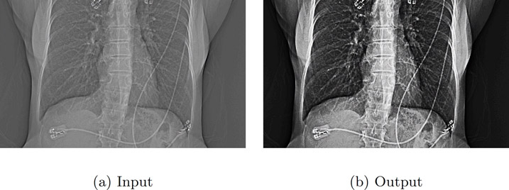
An example of histogram equalization is illustrated in Figure 5.10. Figure 5.10(a) is a CT scout image. The histogram and CDF of the input image are given in Figure 5.10(b). The output image after histogram equalization is given in Figure 5.10(c). The histogram and CDF of the output image are given in Figure 5.10(d). Notice that the histogram of the input image is narrow compared to the range [0, 255]. The leads (bright slender wires running from top to bottom of the image) are not clearly visible in the input image. After histogram equalization, the histogram of the output image is spread out over all the values in the range and subsequently the image is brighter and the leads are visible.

FIGURE 5.10: Example of histogram equalization. Original image reprinted with permission from Dr. Uma Valeti, Cardiovascular Imaging, University of Minnesota.

5.7Contrast Limited Adaptive Histogram Equalization (CLAHE)

In the above histogram equalization method, observe that the output image in 5.10 is too bright. Instead of using the histogram of the whole image, in Contrast Limited Adaptive Histogram Equalization ([Zui94]), the image is divided into small regions and a histogram of each region is computed.

A contrast limit is chosen as a threshold to clip the histogram in each bin, and the pixels above the threshold are not ignored but rather distributed to other bins before histogram equalization is applied.

Let us consider the steps involved:

1.Divide the input image into sub-images of size 8-by-8 (say).

2.Calculate the histogram of each sub-image.

3.Find a PDF as described in Section 5.6.

4.Set a threshold to clip the histograms. Then find the CDF as described in Section 5.6. If the histogram of any bin crosses the clip limit, then the pixels above the clip limit are uniformly distributed to other bins. Since the PDF is clipped, the slope of the CDF will be smaller than the ones in Section 5.6.

5.Apply histogram equalization to each sub-image.

6.Bilinear interpolation is applied to remove artifacts at the boundary of sub-images. We will talk about bilinear interpolation and other interpolation in Chapter 6.

The following is the Python function for the CLAHE filter:

from skimage.exposure import equalize_adapthist
equalize_adapthist(img, clip_limit = 0.02)
 
Necessary arguments:
input is the input image as an ndarray.
 
Optional arguments:
clip_limit is a floating point number between 0 and 1.
A value close to 1 produces higher contrast.

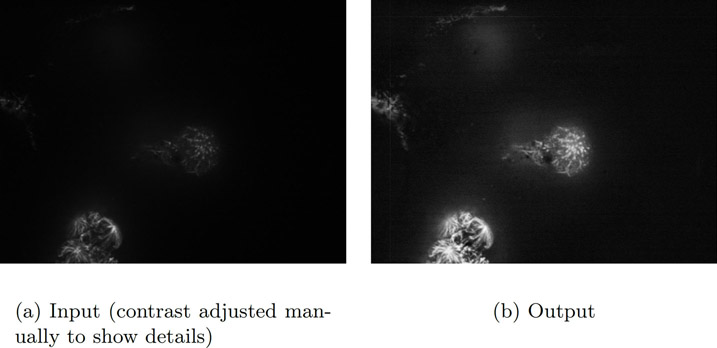
We read the image, ‘embryo.png’ using cv2. As can be seen in Figure 5.11(a), the contrast of the input image is very poor even though it was enhanced manually for publishing purposes. The image is then passed to the equalize_adapthist function with a clip limit of 0.02. The image is scaled to [0, 255] and saved to a file. The output image is displayed in Figure 5.11(b). As can be seen, the output image contrast is better than the input image. Also more details can be seen in the output image compared to the input image.

import cv2
from skimage.exposure import equalize_adapthist
 
img = cv2.imread(’../Figures/embryo.png’)
# Applying Clahe.
img2 = equalize_adapthist(img, clip_limit = 0.02)
 
# Rescaling img2 from 0 to 255.
img3 = img2*255.0
# Saving img3.
cv2.imwrite(’../Figures/clahe_output.png’, img3)

The authors have experienced that CLAHE is particularly useful for image enhancement of MV x-ray images such as seen in radiotherapy.

5.8Contrast Stretching

Contrast stretching is similar in idea to histogram equalization except that the pixel intensities are rescaled using the pixel values instead of probabilities and CDF. Contrast stretching is used to increase the pixel value range by rescaling the pixel values in the input image. Consider an 8-bit image with a pixel value range of [a, b] where a > 0 and b < 255. If a is significantly greater than zero and if b is significantly smaller than 255, then the details in the image may not be visible. This problem can be offset by rescaling the pixel value range to [0, 255], a much larger pixel range.

The contrast stretching transformation, t(i, j) is given by the following equation:

$t (i, j) = 255 * \frac{I (i, j) - a}{b - a}$ $t (i, j) = 255 * \frac{I (i, j) - a}{b - a}$	(5.9)

where I(i, j), a, and b are the pixel intensity at (i, j), the minimum pixel value and the maximum pixel value in the input image respectively. Note that if a = 0 and b = 255, then there will be no change in pixel intensities between the input and the output images.

The image is read and its minimum and maximum values are computed. The image is converted to float, so that the contrast stretching defined in Equation 5.9 can be performed.

import cv2
 
# Opening the image.
im = cv2.imread(’../Figures/hequalization_input.png’)
# Finding the maximum and minimum pixel values
b = im.max()
a = im.min()
print(a,b)
# Converting im1 to float.
c = im.astype(float)
# Contrast stretching transformation.
im1 = 255.0*(c-a)/(b-a+0.0000001)
# Saving im2 as contrast_output.png in
# Figures folder
cv2.imwrite(’../Figures/contrast_output2.png’, im1)

In Figure 5.12(a) the minimum pixel value in the image is 7 and the maximum pixel value is 51. After contrast stretching, the output image (Figure 5.12(b)) is brighter and the details are visible.

FIGURE 5.12: An example of contrast stretching where the pixel value range is significantly different from [0, 255].

In Figure 5.13(a), the minimum pixel value in the image is equal to 0 and the maximum pixel value is equal to 255 so the contrast stretching transformation will not have any effect on this image as shown in Figure 5.13(b).

FIGURE 5.13: An example of contrast stretching where the input pixel value range is same as [0, 255].

5.9Sigmoid Correction

A sigmoid function is defined as

$S (x) = \frac{1.0}{1 + e^{- x * g a i n}}$ $S (x) = \frac{1.0}{1 + e^{- x * g a i n}}$	(5.10)

The function (Figure 5.10) asymptotically reaches 0 for low negative values or reaches 1 asymptotically for high positive values and is always bound between 0 and 1. In the typical definition of a sigmoid function, the value of gain is 1. However, in the case of sigmoid correction, we will use the gain as a hyper-parameter for fine tuning the image enhancement.

For a gain of 0.5, the slope of the linear region around x value of 0 is smaller than the corresponding slope for a gain of 1. Consequently the saturation of pixel values to either 0 or 1 on either end of the spectrum will happen only for points that are farther away from 0. However, for a gain of 2, the saturation point happens close to x = 0. We can use this property to enhance images.

If we choose a gain of 2, then only pixel values (value along x) close to 0 will retain their pixel values while pixel values farther away from 0 will either be saturated to 0 or 1. Hence only a pixel around 0 will be visible with its gray value range.

Instead, if we choose a gain of 0.5, the pixel values farther away from 0 will retain their gray value range and hence we will visualize a large range of pixel values in the image.

In a scikit image, the sigmoid correction is performed using the formula (Equation 5.11),

$S (x) = \frac{1.0}{1 + e^{- (c u t o f f - p i x e l v a l u e) * g a i n}}$ $S (x) = \frac{1.0}{1 + e^{- (c u t o f f - p i x e l v a l u e) * g a i n}}$	(5.11)

where cutoff is the pixel value around which the sigmoid correction is performed. The pixel values must be normalized to [0, 1] before performing sigmoid correction. The cutoff value is the center value of the pixel around which the gray pixel value range is highlighted in the output image.

The following is the Python function for sigmoid correction.

from skimage.exposure import adjust_sigmoid
 
adjust_sigmoid(img1, gain=15)
 
Necessary arguments:
input is the input image as an ndarray.
 
Optional arguments:
gain is a constant multiplier in exponentials power of
 sigmoid function. The default value is 10.

In the code below, the image is read and converted to a numpy array. Then sigmoid correction is applied using the “adjust_sigmoid” function with a gain of 15. Since the cutoff is not specified, the default value of 0.5 will be assumed. A gain of 15 will result in a steep slope in the linear region around 0 in Figure 5.14. Thus only the central pixel values will be highlighted and all other pixels farther away from 0 will be set to either 0 or 1.

import cv2
from skimage.exposure import adjust_sigmoid
 
# Reading the image.
img1 = cv2.imread(’../Figures/hequalization_input.png’)
# Applying Sigmoid correction.
img2 = adjust_sigmoid(img1, gain=15)
# Saving img2.
cv2.imwrite(’../Figures/sigmoid_output.png’, img2)

FIGURE 5.14: Effect of gain in a sigmoid function.

The image in Figure 5.15(a) is sigmoid corrected to produce the output image in Figure 5.15(b). The details of the bones are discernable in the corrected image as opposed to the original image. The choice of the cutoff and gain will determine the quality of the output image.

FIGURE 5.15: Example of Sigmoid correction.

5.10Local Contrast Normalization

Local contrast normalization ([JKRL09]) was developed as part of a computational neural model. The method demonstrates that enhancing the pixel value at a certain location depends only on its neighboring pixels and not the ones farther away from it. The method works by setting the local mean of a pixel to zero and its standard deviation to 1 based on the pixels in the neighborhood.

We begin by creating a difference image (d), computed by finding the difference (Equation 5.12) between the smoothed version of the image and itself. This creates an image whose neighborhood mean is 0. The difference image is then used to compute the standard deviation image (Equation 5.13) after applying a Gaussian smoothing. The final image I_out (Equation 5.14) is created by dividing the difference image by the maximum between the local mean of the standard deviation image and the standard deviation image.

$d = I * σ_{1} - I$ $d = I * σ_{1} - I$	(5.12)

$s = \sqrt{d^{2} * σ_{2}}$ $s = \sqrt{d^{2} * σ_{2}}$	(5.13)

$I_{o u t} = \frac{d}{m a x (m e a n_{s}, s)}$ $I_{o u t} = \frac{d}{m a x (m e a n_{s}, s)}$	(5.14)

where I is the original image, σ₁ and σ₂ are the standard deviations for the Gaussian smoothing, * indicates convolution, and mean_s is the mean of the image s.

The convolution operation works on pixels neighboring a given pixel and hence the filter is called a “local contrast normalization.”

The image used for this example is a DICOM image and is read using the pydicom module. The image is converted to float and scaled to range [0.0, 1.0].

The “localfilter” function implements the local contrast normalization filter. In the function, the input image is smoothed using a Gaussian. A new image called ’d’ is created as a difference between the Gaussian smoothed image and the original image. Since the Gaussian is a weighted mean of the neighborhood pixels, this operation is equivalent to removing the mean from the neighborhood. The mean-corrected image, ’d,’ is then squared to obtain the variance and the square root of the variance provides the standard deviation image ’s’. A new image max_array is created by finding the maximum between the values in image ’s’ and the mean value of image ’s’. The final image ’y’ is created by dividing the image ’d,’ which is similar to mean-corrected image and the standard deviation image, ’max_array’.

import pydicom
import numpy as np
import skimage.exposure as imexp
from matplotlib import pyplot as plt
from scipy.ndimage.filters import gaussian_filter
from PIL import Image
 
def localfilter(im, sigma=(10, 10,)):
  im_gaussian = gaussian_filter(im, sigma=sigma[0])
  d = im_gaussian-im
  s = np.sqrt(gaussian_filter(d*d, sigma=sigma[1]))
  # form an array where all elements have a value of
  mean(s)
  mean_array = np.ones(s.shape)*np.mean(s)
  # find element by element maximum between mean_array
  and s
  max_array = np.maximum(mean_array, s)
  y = d/(max_array+np.spacing(1.0))
  return y
 
file_name = "../Figures/FluroWithDisplayShutter.dcm"
dfh = pydicom.read_file(file_name, force=True)
im = dfh.pixel_array
# convert to float and scale before applying filter
im = im.astype(np.float)
im1 = im/np.max(im)
sigma = (5, 5,)
im2 = localfilter(im, sigma)
# rescale to 8-bit
im3 = 255*(im2-im2.min())/(im2.max()-im2.min())
im4 = Image.fromarray(im3).convert("L")
im4.save(’../Figures/local_normalization_output.png’)
im4.show()

The image in Figure 5.16(b) is a local contrast normalized image produced from the input image in Figure 5.16(a). The details of the bones are discernable in the output image as opposed to the original image. In the bright regions outside the anatomy but inside the field of view, the input image is smooth while the corresponding region in the output image is noisy. This is due to the fact that we are forcing regions with low variance (such as smooth regions) and also regions with high variance to have equal variance. The choice of smoothing is a hyper-parameter that needs to be chosen based on the image being processed.

FIGURE 5.16: Example of local contrast normalization.

The authors have found that this filter works especially well for highlighting high-contrast objects surrounded by low-contrast structures.

5.11Summary

•Image inverse transformation is used to invert the pixel intensities in an image. This process is similar to obtaining a negative of a photograph.

•Power law transformation makes the image brighter for γ < 1 and darker for γ > 1.

•Log transformation makes the image brighter, while the inverse log makes the image darker.

•Histogram equalization is used to enhance the contrast in an image. In this transformation, a narrow range of intensity values will get mapped to a wide range of intensity values.

•Contrast stretching is used to increase the pixel value range by rescaling the pixel values in the input image.

•Sigmoid correction provides a smooth continuous function for enhancing images around a central cutoff.

•Local contrast normalization enhances the pixel value at a certain location based only on its neighboring pixels and not the ones farther away from it.

5.12Exercises

1.Explain briefly the need for image enhancement with some examples.

2.Research a few other image enhancement techniques.

3.Consider an image transformation where every pixel value is multiplied by a constant (K). What will be the effect on the image assuming K < 1, K = 1 and K > 1? What will be the impact on the histogram of the output image in relation to the input image?

4.All the transformations discussed in this chapter are scaled from [0, 1]. Why?

5.The window or level operation allows us to modify the image, so that all pixel values can be visualized. What is the difference between window or level and image enhancement?

Clue: One makes a permanent change to the image while the other does not.

6.An image has all pixel values clustered in the lower intensity. The image needs to be enhanced, so that the small range of the low-intensity maps to a larger range. What operation would you use?

7.In sigmoid correction, the choice of the cutoff and gain will determine the quality of the output image. The readers are recommended to try different settings for the hyper-parameter to understand their effect.

8.In local contrast normalization, the choice of the σ₁ and σ₂ affect the outcome. The readers are recommended to try different values to understand their effect.

..................Content has been hidden....................

You can't read the all page of ebook, please click here login for view all page.

Table of Contents for 5. Image Enhancement

Create new playlist

Sign In

Sign Up

Table of Contents for
5. Image Enhancement