So far we have covered the basics of Python, its scientific modules, and image processing techniques. In this chapter, we begin our journey of learning image acquisition. We will begin the discussion with x-ray generation and detection. We will discuss the various modes in which x-ray interacts with matter. These methods of interaction and detection have resulted in many modes of x-ray imaging such as angiography, fluoroscopy, etc. We complete the discussion with the basics of CT, reconstruction, and artifact removal.
X-rays were discovered by Wilhelm Conrad Rntgen, a German physicist, during his experiment with cathode ray tubes. He called these mysterious rays “x-rays,” the symbol “x” being used in mathematics to denote unknown variables. He found that unlike visible light, these rays passed through most materials and left a characteristic shadow on a photographic plate. His work was published as “On New Kind of Rays” [R95] and was subsequently awarded the first Nobel Prize in Physics in 1901.
Subsequent study of x-rays revealed their true physical nature. They are a form of electromagnetic radiation similar to light, radio waves, etc. They have a wavelength of 10 to 0.01 nanometers. Although they are well known and studied and no longer mysterious, they continue to be referred to as x-rays. Even though the majority of x-rays are man-made using x-ray tubes, they are also found in nature. The branch of x-ray astronomy studies celestial objects by measuring the x-rays emitted.
Since Rntgen’s days, the x-ray has found very widespread use across various fields including radiology, geology, crystallography, astronomy, etc. In the field of radiology, x-rays are used in fluoroscopy, angiography, computed tomography (CT), etc. Today, many non-invasive surgeries are performed under x-ray guidance, providing a new “eye” to the surgeons.
An x-ray imaging system consists of a generator producing a constant and reliable output of x-rays, an object (typically a patient) through which the x-ray traverses, and an x-ray detector to measure the intensity of the rays after passing through the object. We begin with a discussion of the x-ray generation process using an x-ray tube.
An x-ray tube consists of four major parts. They are an anode, a cathode, a tungsten target, and an evacuated tube to hold the three parts together, as shown in Figure 13.1.

The cathode (negative terminal) produces electrons (negatively charged) that are accelerated toward the anode (positive terminal). The filament in the cathode is heated by passing current, which generates electrons by the process of thermionic emission, defined as emission of electrons by absorption of thermal energy. The number of electrons produced is proportional to the current through the filament. This current is generally referred to as “tube current” and is generally measured in “mA” or “milli-amperes.”
Since the interior of an x-ray tube can be hot, a metal with a high melting point such as tungsten is chosen for the filament. Tungsten is also a malleable material, ideal for making fine filaments. The electron produced is focused by the focusing cup, which is maintained at the same negative potential as the cathode. The glass enclosure in which the x-ray is generated is evacuated so that the electrons do not interact with other molecules and can also be controlled independently and precisely. The focusing cup is maintained at a very high potential in order to accelerate the electrons produced by the filament.
The anode is bombarded by the fast-moving electrons. The anode is generally made from copper so that the heat produced by the bombardment of the electrons can be properly dissipated. A tungsten target is fixed to the anode. The fast-moving electrons either knock out the electrons from the inner shells of the tungsten target or are slowed due to the tungsten nucleus. The former results in the characteristic x-ray spectrum while the latter results in the general spectrum or Bremsstrahlung spectrum. The two spectrums together determine the energy distribution in an x-ray and will be discussed in detail in the next section.
The cathode is stationary but the anode can be stationary or rotating. The rotating anode allows even distribution of heat and consequently longer life of the x-ray tube.
There are three parameters that control the quality and quantity of an x-ray. These parameters together are sometimes referred to as an x-ray technique.
They are:
1.Tube voltage measured in kVp.
2.Tube current measured in mA.
3.X-ray exposure time in ms.
In addition, a filter (such as a sheet of aluminum) is placed in the path of the beam, so that lower-energy x-rays are absorbed. This will be discussed in the next section.
The tube voltage is the electric potential between the cathode and the anode. Higher voltage results in increased velocity of the electrons between the cathode and the anode. This increased velocity will produce high-energy x-rays while a lower voltage results in lower-energy x-rays and consequently a noisier image. The tube current determines the number of electrons being emitted. This in turn determines the quantity of x-rays. The exposure time determines the time for which the object or patient is exposed to x-rays. This is generally the time the x-ray tube is operating.
13.3.2X-Ray Generation Process
The x-ray generated by the tube does not contain photons of a single energy. It instead consists of a large range of energy. The relative number of photons at each energy level is measured to generate a histogram. This histogram is called the spectral distribution or spectrum for short. There are two types of x-ray spectrums [CDM84b]. They are the general radiation or Bremsstrahlung “Braking” spectrum, which is a continuous radiation, and the characteristic spectrum, a discrete entity as shown in Figure 13.2.
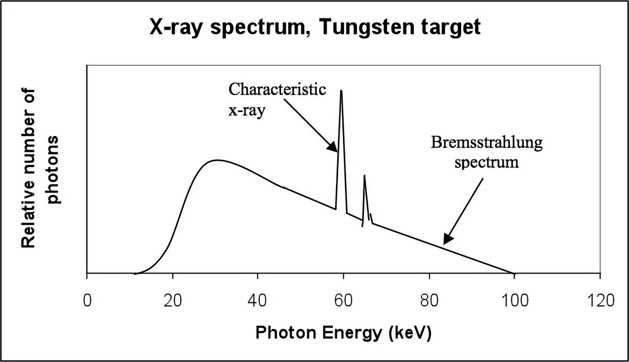
FIGURE 13.2: X-ray spectrum illustrating characteristic and Bremsstrahlung.
When the fast-moving electrons produced by the cathode move very close to the nucleus of the tungsten atom (Figure 13.3), the electrons decelerate and the loss of energy is emitted as radiation. Most of the radiation is at a higher wavelength (or lower energy) and hence is dissipated as heat. The electrons are not decelerated completely by one tungsten nucleus, and hence at every stage of deceleration, radiation of lower wavelength or higher energy is emitted. Since the electrons are decelerated or “braked” in the process, this spectrum is referred to as Bremsstrahlung or braking spectrum. This spectrum gives the x-ray spectrum its wide range of photon energy levels.

From the energy equation, we know that
(13.1) |
|---|
where h = 4.135 * 10−18 eV s is Planck’s constant, c = 3*108 m/s is the speed of light, and λ is the wavelength of the x-ray measured in Angstroms (Å= 10−10m). The product of h and c is 12.4 *10−10 keV m. When E is measured in keV, the equation simplifies to
(13.2) |
|---|
The inverse relationship between E and λ implies that a shorter wavelength produces a higher-energy x-ray and vice versa. For an x-ray tube powered at 112 kVp, the maximum energy that can be produced is 112 keV and hence the corresponding wavelength is 0.11 Å. This is the shortest wavelength and also the highest energy that can be achieved during the production of Bremsstrahlung spectrum. This is the right-most point in the graph in Figure 13.2. However, most of the x-ray will be produced at much higher wavelength and consequently lower energy.
The second type of radiation spectrum (Figure 13.4) results from a tungsten electron in its orbit interacting with the emitted electron. This is referred to as characteristic radiation, as the peaks in the histogram of the spectrum are characteristic of the target material.

The fast-moving electrons eject the electron from the k-shell (inner shell) of the tungsten atom. Since this shell is unstable due to the ejection of the electron, the vacancy is filled by an electron from the outer shell. This is accompanied by release of x-ray energy. The energy and wavelength of the electron are dependent on the binding energy of the electron whose position is filled. Depending on the shell, these characteristic radiations are referred as K, L, M and N characteristic radiation and are shown in Figure 13.2.
X-rays do not just interact with the tungsten atom, they can interact with any atom in their path. Thus, a molecule of oxygen in the path will be ionized by an x-ray knocking out its electron. This could change the x-ray spectrum and hence the x-ray generator tube is maintained at vacuum.
Once the x-ray is generated, it is allowed to pass through a patient or an object. The material in the object reduces the intensity of the x-ray either by absorption or deflection of photons in the beam. This process is referred to as attenuation. If there are multiple materials, each of the materials can absorb or deflect the x-ray and consequently reduce its intensity.
The attenuation is quantified by using a linear attenuation coefficient (μ), defined as the attenuation per centimeter of the object. The attenuation is directly proportional to the distance traveled and the incident intensity. The intensity of the x-ray beam after attenuation is given by the Lambert-Beer law (Figure 13.5) expressed as
(13.3) |
|---|
where I0 is the initial x-ray intensity, I is the exiting x-ray intensity, μ is the linear attenuation coefficient of the material, and δx is the thickness of the material. The law also assumes that the input x-ray intensity is mono-energetic or monochromatic.
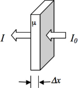
FIGURE 13.5: Lambert-Beer law for monochromatic radiation and for a single material.
Monochromatic radiation is characterized by photons of single intensity, but in reality all radiations are polychromatic and have photons of varying intensity with spectra similar to Figure 13.2. Polychromatic radiation is characterized by photons of varying energy (quality and quantity), with the peak energy being determined by the peak kilovoltage (kVp).
When polychromatic radiation passes through matter, the longer wavelengths and lower energy are preferentially absorbed. This increases the mean energy of the beam. This process of increased mean energy of the beam is referred to as “beam hardening.”
In addition to the attenuation coefficient, the characteristics of a material under x-ray can also be defined using the half-value layer. This is defined as the thickness of material needed to reduce the intensity of the x-ray beam by half. So from Equation 13.3 for a thickness δx = HVL (half value layer),
(13.4) |
|---|
Hence,
(13.5) |
|---|
(13.6) |
|---|
(13.7) |
|---|
For a material with linear attenuation coefficient of 0.1/cm, the HVL is 6.93 cm. This implies that when a monochromatic beam of x-ray passes through the material, its intensity drops by half after passing through 6.93 cm of that material.
The HVL depends not only on the material being studied but also on the tube voltage. High tube voltage produces a smaller number of low-energy photons, i.e., the spectrum in Figure 13.2 will be shifted to the right. The mean energy will be higher and the beam will be harder. This hardened beam can penetrate material without a significant loss of energy. Thus, the HVL will be high for high x-ray tube voltage. This trend can be seen in the HVL of aluminum at different tube voltages given in Table 13.1.
TABLE 13.1: Relationship between kVp and HVL.
|
kVp |
HVL(mm of Al) |
|
50 |
1.9 |
|
75 |
2.8 |
|
100 |
3.7 |
|
125 |
4.6 |
|
150 |
5.4 |
13.4.2Lambert-Beer Law for Multiple Materials
For an object with n materials (Figure 13.6), the Lambert-Beer law is applied in cascade,
(13.8) |
|---|

When the logarithm of the intensities is taken, for a continuous domain we obtain
(13.9) |
|---|
Using this equation, we see that the value p, the projection image expressed in energy intensity, corresponding to the digital value at a specific location in that image, is simply the sum of the product of attenuation coefficients and thicknesses of the individual components. This is the basis of image formation in x-ray. The inverse of this summation process is the CT reconstruction that will be discussed shortly.
13.4.3Factors Determining Attenuation
The energy of the beam is one of the factors that determines the amount of attenuation. As we have seen earlier, lower-energy beams get preferentially absorbed compared to higher-energy beams.
The density of a substance through which x-rays pass makes a significant contribution to the attenuation. A higher-density substance like bone attenuates x-rays more than a lower-density substance like tissue. Also different types of tissue have different densities and hence different attenuation, resulting in different contrast on the x-ray image. The physical characteristic that determines the attenuation is the number of electrons per gram in the material. A material with a higher number of electrons per gram has a higher probability of interacting with the x-rays. The number of electrons per gram is given by
(13.10) |
|---|
where N is the number of electrons per gram, N0 = 6*1023 is Avogadro’s number, Z is the atomic number, and A is the atomic weight of the substance. Since Avogadro’s number is a constant, the number of electrons per gram is dependent only on Z and A.
So far, we have discussed x-ray generation using an x-ray tube, the shape of the x-ray spectrum, and also studied the change in x-ray intensity as it traverses a material due to attenuation. These attenuated x-rays have to be converted to a human-viewable form. This conversion process can be achieved by exposing them on a photographic plate to obtain an x-ray image or viewing them using a TV screen or converting to a digital image, all using the process of x-ray detection. There are three different types of x-ray radiation detectors in practice, namely ionization, fluorescence, and absorption.
1.Ionization detection
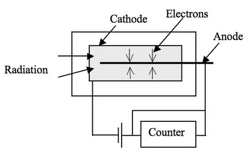
In the ionization detector, the x-rays ionize the gas molecules in the detector and by measuring the ionization, the intensity of the x-ray is measured. An example of such a detector is the Geiger Muller counter [Mac83] shown in Figure 13.7. These detectors are used to measure the intensity of radiation and are not used for creating x-ray images.
2.Scintillation detection
There are different types of scintillation detectors. The most popular are the Image Intensifier (II) and Flat Panel Detector (FPD). In an II, [Mac83], [CDM84b], [FH00], the x-rays are converted to electrons that are accelerated to increase their energy. The electrons are then converted back to light and are viewed on a TV or a computer screen. In the case of an FPD, the x-rays are converted to visible light and then to electrons using a photo diode. The electrons are recorded using a camera. In both the II and FPD, the process of converting x-ray to electron and accelerating it is used for improving the image gain. Modern technology has allowed the creation of a large FPD with very high quality and hence the FPD is rapidly replacing the II. Also, FPD occupies significantly less space than the II. We will discuss both in detail.
The II (Figure 13.8) consists of an input phosphor and photocathode, an electrostatic focusing lens, an accelerating anode and an output fluorescent screen. The x-ray beam passes through the patient and enters the II through the input phosphor. The phosphor generates light photons after absorbing the x-ray photons. The light photons are absorbed by the photocathode and electrons are emitted. The electrons are then accelerated by a potential difference toward the anode. The anode focuses the electron onto an output fluorescence screen that emits the light that will be displayed using a TV screen, recorded on an x-ray film, or recorded by a camera onto a computer.
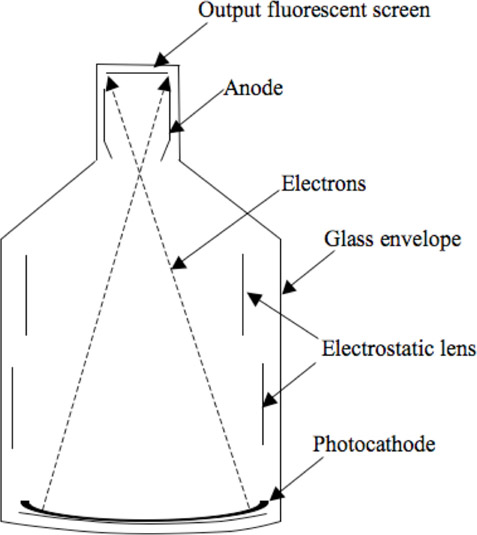
The input phosphor is made of cesium iodide (CsI) and is vapor deposited to form a needlelike structure that prevents diffusion of light and hence improves resolution. It also has greater packing density and hence higher conversion efficiency, even with smaller thickness (needed for good spatial resolution). A photocathode emits electrons when light photons are incident on it. The anode accelerates the electrons. The higher the acceleration the better is the conversion of electrons to light photons at the output phosphor. The input phosphor is curved, so that electrons travel the same length toward the output phosphor. The output fluorescent screen is silver-activated zinc-cadmium sulfide. The output can be viewed using a series of lenses on a TV or it can be recorded on a film.
The field size is changed by changing the position of the focal point, the point of intersection for the left and right electron beams. This is achieved by increasing the potential in the electrostatic lens. Lower potential results in the focus being close to the anode and hence the full view of the anatomy is exposed to the output phosphor. At higher potential, the focus moves away from the anode and hence only a portion of the input phosphor is exposed to the output phosphor. In both cases, the size of the input and output phosphors remains the same but in the smaller mode, a portion of the image from the input phosphor is removed from the view due to a farther focal point.
In a commercial x-ray unit, these sizes are specified in inches. A 12-inch mode will cover a larger anatomy while a 6-inch mode will cover a smaller anatomy. Exposure factors are automatically increased for smaller II modes to compensate for the decreased brightness from minification.
Since the electrons travel large distances during their journey from photocathode to anode, they are affected by the earth’s magnetic field. The earth’s magnetic field changes even for small motions of the II and hence the electron path gets distorted. The distorted electron path produces a distorted image on the output fluorescent screen. The distortion is not uniform but increases near the edge of the II. Hence the distortion is more significant for a large II mode than for a smaller II mode. The distortions can be removed by careful design and material selection or more preferably using image processing algorithms.
13.5.3Flat Panel Detector (FPD)
The FPD (Figure 13.9) consists of a scintillation detector, a photo diode, an amorphous silicon, and a camera. The x-ray beam passes through the patient and enters the FPD through the scintillation detector. The detector generates light photons after absorbing the x-ray photons. The light photons are absorbed by the photo diode and electrons are emitted. The electrons are then absorbed by the amorphous silicon layer, which produces an image that is recorded using a charge-couple device (CCD) camera.

Similar to the II, the scintillation detector is made of cesium iodide (CsI) or gadolinium oxysulfide and is vapor deposited to form a needle-like structure, which acts like fiber optic cable and prevents diffusion of light and improves resolution. The CsI is generally coupled with amorphous silicon, as CsI is an excellent absorber of x-ray and emits light photons at a wavelength best suited for amorphous silicon to convert to electrons.
The II needs extra length to allow accelerating of the electron, while the FPD does not. Hence the FPD occupies significantly less space compared to the II. The difference becomes significant as the size of the detector increases. IIs are affected by the earth’s magnetic field while such problems do not exist for the FPD. Hence the FPD can be mounted on an x-ray machine and be allowed to rotate around the patient without distorting the image. Although the II suffers from some disadvantages, it is simpler in its construction and electronics.
The II or FPD can be bundled with an x-ray tube, a patient table, and a structure to hold all these parts together, to create an imaging system. Such a system could also be designed to revolve around the patient table axis and provide images in multiple directions to aid diagnosis or medical intervention. Examples of such systems, fluoroscopy and angiography, are discussed below.
The first-generation fluoroscope [Mac83],[CDM84b] consisted of a fluoroscopic screen made of copper-activated cadmium sulfide that emitted light in the yellow-green spectrum of visible light. The image was so faint that the viewing was carried out in a dark room, with the doctors adapting their eyes to the dark prior to examination. Since the intensity of fluorescence was less, rod vision in the eye was used and hence the ability to differentiate shades of gray was also poor. These problems were alleviated with the invention of the II discussed earlier. The II allowed intensification of the light emitted by the input phosphor so that it could safely and effectively be used to produce a system (Figure 13.10) that could generate and detect x-rays and also produce images that can be studied using TVs and computers.

FIGURE 13.10: Fluoroscopy machine. Original image reprinted with permission from Siemens AG.
A digital angiographic system [Mac83], [CDM84b] consists of an x-ray tube, a detector such as a II or FPD and a computer to control the system and record or process the images. The system is similar to fluoroscopy except that it is primarily used to visualize blood vessels opacified using a contrast. The x-ray tube must have a larger focal spot and also provide a constant output over time. The detector must also provide a constant acceleration voltage to prevent variation in gain during acquisition. A computer controls the whole imaging chain.
The computing system also performs digital subtraction in the case of digital subtraction angiography (DSA) [CDM84b] on the obtained images. In the DSA process, the computer controls the x-ray technique so that uniform exposure is obtained across all images. The computer obtains the first set of images without the injection of contrast and stores them as a mask image. Subsequent images obtained under the injection of contrast are stored and subtracted from the mask image to obtain the image with the blood vessel alone.
The fluoroscopy and angiography discussed so far produce a projection image, which is a shadow of part of the body under x-ray. These systems provide a planar view from one direction and may also contain other organs or structures that impede the ability to make a clear diagnosis. CT on the other hand, provides a slice through the patient and hence offers an unimpeded view of the organ of interest. In CT, a series of x-ray images are acquired all around the object or patient. A computer then processes these images to produce a map of the original object using a process called reconstruction. Sir Godfrey N. Hounsfield and Dr. Allan McCormack developed CT independently and later shared the Nobel Prize for Physiology in 1979. The utility of this technique became so apparent that an industry quickly developed around it, and it continues to be an important diagnostic tool for physicians and surgeons. For more details refer to [Bus00],[Hen83],[Kal00].
The basic principle of reconstruction is that the internal structure of an object can be computed from multiple projections of that object. In the case of CT reconstruction, the internal structure being reconstructed is the spatial distribution of the linear attenuation coefficients (μ) of the imaged object. Mathematically, Equation 13.9 can be inverted by the reconstruction process to obtain the distribution of the attenuation coefficients.
In clinical CT, the raw projection data is often a series of 1D vectors of x-ray projection obtained at various angles for which the 2D reconstruction yields a 2D attenuation coefficient matrix. In the case of 3D CT, a series of 2D images obtained at various angles are used to obtain a 3D distribution of the attenuation coefficient. For the sake of simplicity, the reconstructions discussed in this chapter will focus on 2D reconstructions and hence the projection images are 1D vector unless otherwise specified.
The original method used for acquiring CT data used parallel-beam geometry such as is shown in Figure 13.11. As shown in the figure, the paths of the individual rays of x-ray from the source to the detector are parallel to each other. An x-ray source is collimated to yield a single x-ray beam, and the source and detector are translated along the axis perpendicular to the beam to obtain the projection data (a single 1D vector for a 2D CT slice). After the acquisition of one projection, the source-detector assembly is rotated and subsequent projections are obtained. This process is repeated until a 180-degree projection is obtained. The reconstruction is obtained using the central slice theorem or the Fourier slice theorem [KS88]. This method forms the basis for many CT reconstruction techniques.

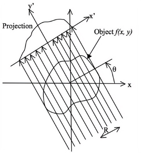
Consider the object shown in Figure 13.12 to be reconstructed. The original coordinate system is x-y and when the detector and x-ray source are rotated by an angle θ, then their coordinate system is defined by x′ − y′. In this figure, R is the distance between the iso-center (i.e., center of rotation) and any ray passing through the object. After logarithmic conversion, the x-ray projection at an angle (θ) is given by
(13.11) |
|---|
where δ is the Dirac-Delta function [Bra99].
The Fourier transform of the distribution is given by
(13.12) |
|---|
where u and v are frequency components in perpendicular directions. Expressing u and v in polar coordinates, we obtain u = νcosθ and v = νsinθ , where ν is the radius and θ is the angular position in the Fourier space.
Substituting for u and v and simplifying yields,
(13.13) |
|---|
The equation can be rewritten as
(13.14) |
|---|
Rearranging the integrals yields,
(13.15) |
|---|
From Equation 13.11, we can simplify the above equation as
(13.16) |
|---|
where FT( ) refers to the Fourier transform of the enclosed function. Equation 13.16 shows that the radial slice along an angle θ in the 2D Fourier transform of the object is the 1D Fourier transform of the projection data acquired at that angle θ. Thus, by acquiring projections at various angles, the data along the radial lines in the 2D Fourier transform can be obtained. Note that the data in the Fourier space is obtained using polar sampling. Thus, either a polar inverse Fourier transform must be performed or the obtained data must be interpolated onto a rectilinear Cartesian grid so that Fast Fourier Transform (FFT) techniques can be used.
However, another approach can also be taken. Again, f(x, y) is related to the inverse Fourier transform, i.e.,
(13.17) |
|---|
By using a polar coordinate transformation, u, v can be written as u = cosθ and v = sinθ. To effect a coordinate transformation, the Jacobian is used and is given by
(13.18) |
|---|
Hence,
(13.19) |
|---|
Thus,
(13.20) |
|---|
Using Equation 13.16, we can obtain
(13.21) |
|---|
(13.22) |
|---|
(13.23) |
|---|
The term in the braces is the filtered projection, which can be obtained by multiplying the Fourier transform of the projection data by |ν| in the Fourier space or equivalently by performing a convolution of the real space projections and the inverse Fourier transform of the function |ν|. Because the function looks like a ramp, the filter generated is commonly called the “ramp filter.”
Thus,
(13.24) |
|---|
where FT(R, θ) is the filtered projection data at location R acquired at angle θ is given by
(13.25) |
|---|
Once the convolution or filtering is performed, the resulting data is reconstructed using Equation 13.25. This process is referred to as the filtered back projection (FBP) technique and is the most commonly used technique in practice.
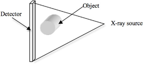
The fan-beam CT scanners (Figure 13.13) have a bank of detectors, with all detectors being illuminated by x-rays simultaneously from every projection angle. Since the detector acquires images in one x-ray exposure, it eliminates the translation at each angle. Since translation is eliminated, the system is mechanically stable and faster. However, x-rays scattered (we will discuss scatter correction later) by the object reduce the contrast in the reconstructed images compared to parallel-beam reconstruction. But these machines are still popular due to faster acquisition time, which allows reconstruction of a moving object, like slices of the heart, in one breath-hold. The images acquired using fan-beam scanners can be reconstructed using a rebinning method that converts fan-beam data into parallel-beam data and then uses the central slice theorem for reconstruction. Currently, this approach is not used and is replaced by a direct fan-beam reconstruction method based on filtered back-projection.
A fan-beam detector with one row of detecting elements produces one CT slice. The current generations of fan-beam CT machines have multiple detector rows and can acquire 8, 16, 32 slices, etc., in one rotation of the object and are referred to as multi-slice CT machines. The benefit is faster acquisition time compared to single slice and also covering a larger area in one exposure. With the advent of multi-slice CT machines, a whole-body scan of the patient can also be obtained.
Figure 13.14 is the axial slice of the region around the human kidney. It is one of the many slices of the whole body scan shown in the montage in Figure 13.15. These slices were converted into a 3D object (Figure 13.16) using MimicsTM [Mat20a].
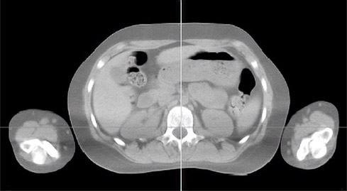
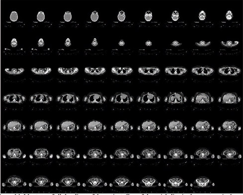
FIGURE 13.15: Montage of all the CT slices of the human kidney region.

FIGURE 13.16: 3D object created using the axial slices shown in the montage. The 3D object in green is superimposed on the slice information for clarity.
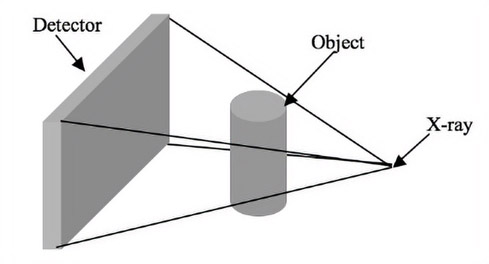
Cone-beam acquisition or CBCT (Figure 13.17) consists of 2D detectors instead of 1D detectors used in the parallel and fan-beam acquisitions. As with fan-beam, the source and detector rotate relative to the object, and the projection images are acquired. The 2D projection images are then reconstructed to obtain 3D volume. Since a 2D region is imaged, cone-beam-based volume acquisition makes use of x-rays that otherwise would have been blocked. The advantages are potentially faster acquisition time, better pixel resolution, and isotropic (same voxel size in x, y and z directions) voxel resolution. The most commonly used algorithm for cone-beam reconstruction is the Feldkamp algorithm [FDK84], which assumes a circular trajectory for the source and flat detector and is based on filtered back-projection.
Micro-tomography (commonly known as industrial CT scanning), like tomography, uses x-rays to create cross-sections of a 3D object that later can be used to re-create a virtual model without destroying the original model. The term micro is used to indicate that the pixel sizes of the cross-sections are in the micrometer range. These pixel sizes have also resulted in the terminology micro-computed tomography, micro-CT, micro-computer tomography, high-resolution x-ray tomography, and similar terminologies. All of these names generally represent the same class of instruments.
This also means that the machine is much smaller in design compared to the human version and is used to image smaller objects. In general, there are two types of scanner setups. In the first setup, the x-ray source and detector are typically stationary during the scan while the animal or specimen rotates. In the second setup, much more like a clinical CT scanner, the animal or specimen is stationary while the x-ray tube and detector rotate.
The first x-ray micro-CT system was conceived and built by Jim Elliott in the early 1980s [ED82]. The first published x-ray micro-CT images were reconstructed slices of a small tropical snail, with pixel size about 50 micrometers, which appeared in the same paper.
Micro-CT is generally used for studying small objects such as polymers, plastics, micro devices, electronics, paper, and fossils. It is also used in the imaging of small animals such as mice, or insects, etc.
The HU is the system of units used in CT that represents the linear attenuation coefficient of an object. It provides a standard way of comparing images acquired using different CT machines. The conversion of reconstructed pixel values to HUs is a linear transformation given by
(13.26) |
|---|
where μ is the linear attenuation coefficient of the object and μw is the linear attenuation coefficient of water. Thus, water has an HU of 0 and air has an HU of −1000 since μ of air is 0.
The following are the steps to obtain the HU equivalent of a reconstructed image:
•A water phantom consisting of a cylinder filled with water is reconstructed using the same x-ray technique as the reconstructed patient slices.
•The attenuation coefficient of water and air (present outside the cylinder) is measured from the reconstructed slice.
•A linear fit is established with the HU of water (0) and air (−1000) being the ordinate and the corresponding linear attenuation coefficients measured from the reconstructed image being the abscissa.
•Any patient data reconstructed is then mapped to HUs using the determined linear fit.
Since the CT data is calibrated to HUs, the data in the images acquires meaning not only qualitatively but also quantitatively. Thus, an HU number of 1000 for a given pixel or voxel represents quantitatively a bone in an object.
Unlike MRI, microscopy, ultrasound, etc., due to use of HUs for calibration, CT measurement is a map of a physical property of the material. This is handy while performing image segmentation, as the same threshold or segmentation technique can be used for measurements from various patients at various intervals and conditions. It is also useful in performing quantitative CT, a process of measuring the property of the object using CT.
In all the prior discussions, it was assumed that the x-ray beam is mono-energetic. It was also assumed that the geometry of the imaging system is well characterized, i.e., there is no change in the orbit that the imaging system follows with reference to the object. However, in current clinical CT technology, the x-ray beam is not mono-energetic and the geometry is not well characterized. This results in errors in the reconstructed image that are commonly referred as artifacts, defined as any discrepancy between the reconstructed value in the image and the true attenuation coefficients of the object [Hsi03]. Since the definition is broad and can encompass many things, discussions of artifacts are generally limited to clinically significant errors. CT is more prone to artifacts than conventional radiography, as multiple projection images are used. Hence errors in different projection images cumulate to produce artifacts in the reconstructed image. These artifacts could annoy radiologists or in some severe cases hide important details that could lead to misdiagnosis.
Artifacts can be eliminated to some extent during acquisition. They can also be removed by pre-processing projection images or post-processing the reconstructed images. There are no generalized techniques for removing artifacts and hence new techniques are devised depending on the application, anatomy, etc. Artifacts cannot be completely eliminated but can be reduced by using correct techniques, proper patient positioning, and improved design of CT scanners, or by software provided with the CT scanners.
There are many sources of error in the imaging chain that can result in artifacts. They can generally be classified as artifacts due to the imaging system or artifacts due to the patient. In the following discussion, the geometric alignment, offset and gain correction are caused by the imaging system while the scatter and beam-hardening artifacts are caused by the nature of object or patient being imaged.
13.9.1Geometric Misalignment Artifacts
The geometry of a CBCT system is specified using six parameters, namely the three rotation angles (angles corresponding to u, v and w axes in Figure 13.18) and three translations along the principal axis (u, v, w in Figure 13.18). An error in these parameters can result in a ring artifact [CMSJ05],[FH00], double wall artifact, etc., which are visual and hence cannot be misdiagnosed as a pathology. However, very small errors in these parameters can result in blurring of edges and hence misdiagnosis of the size of the pathology, or shading artifacts that could shift the HU number. Hence these parameters must be determined accurately and corrected prior to reconstruction.

In our previous discussion, we learned that an incident x-ray photon ejects an electron from the orbit of the atom, and consequently a low-energy x-ray photon is scattered from the atom. The scattered photon travels at an angle from its incident direction (Figure 13.19). These scattered radiations are detected but arrive at the detector like the primary radiation. They reduce the contrast of the image and produce blurring. The effect of scatter in the final image is different for conventional radiography and CT. In the case of radiography, the images have poor contrast but in the case of CT, the logarithmic transformation results in a non-linear effect.

Scatter also depends on the type of image acquisition technique. For example, fan-beam CT has less scatter compared to a cone-beam CT due to the smaller height of the beam.
One of the methods to reduce scatter is the air gap technique. In this technique, a large air-gap is maintained between the patient and the detector. Since the scattered radiation at a large angle from the incident direction cannot reach the detector, it will not be used in the formation of the image. It is not always possible to provide an air gap between the patient and the detector, so grids or post-collimators [CDM84b],[Hsi03] made of lead strips are used to reduce scatter. The grids contain space which corresponds to the photo-detector being detected. The scattered radiation arriving at a large angle will be absorbed by lead and only primary radiations arriving at a small angle from the incident direction is detected. The third approach is software correction [LK87],[OFKR99]. Since scatter is a low-frequency structure causing blurring, it can be approximated by a number estimated using the beam-stop technique [Hsi03]. This, however, does not remove the noise associated with the scatter.
13.9.3Offset and Gain Correction
Ideally, the response of a detector must remain constant for a constant x-ray input at any time. But due to temperature fluctuations during acquisition, non-idealities in the production of detectors and variations in the electronic readouts, a non-linear response may be obtained in the detectors. These non-linear responses result in the output of that detector cell being inconsistent with reference to all the neighboring detector pixels. During reconstruction, the non-linear responses produce ring artifacts [Hsi03] with their center being located at the iso-center. These circles may not be confused with human anatomy, as there are no parts which form a perfect circle, but they degrade the quality of the image and hide details and hence need to be corrected. Moreover the detector produces some electronic readout, even when the x-ray source is turned off. This readout is referred to as “dark current” and needs to be removed prior to reconstruction.
Mathematically the flat field and zero offset corrected image (IC) is given by
(13.27) |
|---|
where IA is the acquired image, ID is the dark current image, IF is flat field image, which is acquired at the same technique as the acquired image with no object in the beam. The ratio of the differences is multiplied by the average value of (IF − ID) for gain normalization. This process is repeated for every pixel. The dark field images are to be acquired before each run, as they are sensitive to temperature variations. Other software-based correction techniques based on image processing are also used to remove the ring artifacts. They can be classified as pre-processing and post-processing techniques. The pre-processing techniques are based on the fact that the rings in the reconstructed images appear as vertical lines in the projection space. Since no feature in an object except those at the iso-center can appear as vertical lines, the pixels corresponding to vertical lines can be replaced using estimated pixel values. Even though the process is simple, the noise and complexity of human anatomy present a big challenge in the detection of vertical lines. Another correction scheme is the post-processing technique [Hsi03]. The rings in the reconstructed images are identified and removed. Since ring detection is primarily an arc detection technique, it could result in over-correcting the reconstructed image for features that look like arcs. So in a supervised ring removal technique, inconsistencies across all views are considered. To determine the position of pixels corresponding to a given ring radius, a mapping that depends on the location of source, object and image is used.
The spectrum (Figure 13.2) does not have a unique energy but has a wide range of energies. When such an energy spectrum is incident on a material, the lower energy gets attenuated faster as it is preferentially absorbed than the higher-energy. Hence a polychromatic beam becomes harder or richer in higher-energy photons as it passes through the material. Since the reconstruction process assumes an “ideal” mono-chromatic beam, the images acquired using a polychromatic beam produce cupping artifacts [BK04]. The cupping artifact is characterized by a radial increase in intensity from the center of the reconstructed image to its periphery. Unlike ring artifacts, this artifact presents difficulty, as it can mimic some pathology and hence can lead to misdiagnosis. The cupping artifacts also shift the intensity values and hence present difficulty in quantification of the reconstructed image data. They can be reduced by hardening the beam prior to reaching the patient, using a filter made of aluminum, copper, etc. Algorithmic approaches [BK04] for reducing these artifacts have also been proposed.
Metal artifacts are caused by the presence of materials that have a high attenuation coefficient when compared to pathology in the human body. These include surgical clips, biopsy needles, tooth fillings, implants, etc. Due to their high attenuation coefficient, metal artifacts produce beam-hardening artifacts (Figure 13.20) and are characterized by streaks emanating from the metal structures. Hence techniques used for removing beam hardening can be used to reduce these artifacts.
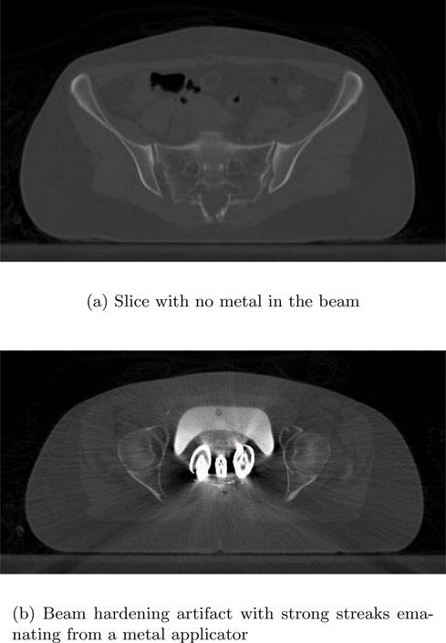
In Figure 13.20, the top image is a slice taken at a location without any metal in the beam. The bottom image contains an applicator. The beam hardening causes a streaking artifact that not only renders the metal poorly reconstructed but also adds streaks to nearby pixels and hence makes diagnosis difficult.
Algorithmic approaches [Hsi03], [JS78], [WSOV96] to reducing these artifacts have been proposed. A set of initial reconstructions is performed without any metal artifact correction. From the reconstructed image, the location of metal objects is then determined. These objects are then removed from the projection image to obtain a synthesized projection. The synthesized projection is then reconstructed to obtain a reconstructed image without metal artifacts.
•A typical x-ray and CT system consists of an x-ray tube, detector and a patient table.
•X-ray is generated by bombarding high-speed electrons on a tungsten target. A spectrum of x-ray is generated. There are two parts to the spectrum: Bremsstrahlung or braking spectrum and the characteristic spectrum.
•The x-ray passes through a material and is attenuated. This is governed by the Lambert-Beer law.
•The x-ray after passing through a material is detected using either an ionizing detector or a scintillation detector such as the II or FPD.
•X-ray systems can be either fluoroscopic or angiographic.
•A CT system consists of an x-ray tube and detector, that are rotated around the patient to acquire multiple images. These images are reconstructed to obtain the slice through a patient.
•The central slice theorem is an analytical technique for reconstructing images. Based on this theorem, it can be proven that the reconstruction process consists of filtering and then back-projection.
•The Hounsfield unit is the unit of measure in CT. The unit is a map of the attenuation coefficient of the material.
•CT systems suffer from various artifacts such as misalignment artifact, scatter artifact, beam hardening artifact, and metal artifact.
1.Describe briefly the various parameters that control the quality of x-ray or CT images.
2.An x-ray tube has an acceleration potential of 50kVp. What is the wavelength of the x-ray?
3.Describe the difference in the detection mechanism between II and FPD. Specifically describe the advantages and disadvantages.
4.Allan M. Cormack and Godfrey N. Hounsfield won the 1979 Nobel Prize for creation of CT. Read their Nobel acceptance speech and understand the improvement in contrast and spatial resolution of the images described compared to current clinical images.
5.What is the HU value of a material whose linear attenuation coefficient is half of the linear attenuation coefficient of water?
6.A metal artifact causes significant distortion of an image both in structure and HU value. Using the list of papers in the references, summarize the various methods.