
Magnetic Resonance Imaging (MRI) is built on the same physical principle as Nuclear Magnetic Resonance (NMR), which was first described by Dr. Isidor Rabi in 1938 and for which he was awarded the Nobel Prize in Physics in 1944. In 1952, Felix Bloch and Edward Purcell won the Nobel Prize in Physics for demonstrating the use of the NMR technique in various materials.
It took a few more decades to apply the NMR principle to imaging the human body. Paul Lauterbur developed the first MRI machine that generated 2D images. Peter Mansfield expanded on Paul Lauterbur’s work and developed mathematical techniques that are still part of MRI image creation. For their work, Peter Mansfield and Paul Lauterbur were awarded the Nobel Prize in Physics in 2003.
MRI has developed over the years as one of the most commonly used diagnostic tools by physicians all over the world. It is also popular due to the fact that it does not use ionizing radiation. It is superior to CT for imaging tissue, due to its better tissue contrast.
Unlike the physics and workings of CT, MRI physics is more involved and hence this chapter is arranged differently than the CT chapter. In the x-ray and CT chapter, we began with the construction and generation of x-ray, then discussed the material properties that govern x-ray imaging, and finally discussed x-ray detection and image formation. However, in this chapter we begin the discussion with the various laws that govern NMR and MRI. This includes Faraday’s law of electromagnetic induction, Larmor frequency, and the Bloch equation. This is followed by material properties such as T1 and T2 relaxation times and the gyromagnetic ratio and proton density that govern MRI imaging. This is followed by sections on NMR detection and finally MRI imaging. With all the physics understood, we discuss the construction of an MRI machine. We conclude with the various modes and potential artifacts in MRI imaging. Interested readers can find more details in [Bus88],[CDM84a],[DKJ06],[Hor95],[Mac83],[MW98],[McR03],[Spl10],[Wes09].
14.2Laws Governing NMR and MRI
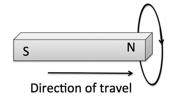
Faraday’s law is the basic principle behind electric motors and generators. It is also part of today’s electric and electric-hybrid cars. It was discovered by Michael Faraday in 1831 and was correctly theorized by James Clerk Maxwell. It states that current is induced in a coil at a rate at which the magnetic flux changes. In Figure 14.1, when the magnet is moved in and out of the coil in the direction shown, a current is induced in the coil in the direction shown. This is useful for electrical power generation, where the flux of the magnetic field is achieved by rotating a powerful magnet inside the coil. The power for the motion is obtained using mechanical means such as potential energy of water (hydroelectric), chemical energy of diesel (diesel engine power plants), etc.
The converse is also true. When a current is passed through a closed circuit coil, it will cause the magnet to move. By constricting the motion of the magnet to rotation, an electric motor can be created. By suitably wiring the coils, an electric generator can thus become an electric motor. In the former, the magnet is rotated to induce current in the coil while in the latter, a current passed through the coil rotates the magnet.
MRI and NMR use electric coils for excitation and detection. During the excitation phase, the current in the coil will induce a magnetic field that causes the atoms to align in the direction of the magnetic field. During the detection phase, the change in the magnetic field is detected by measuring the induced current.
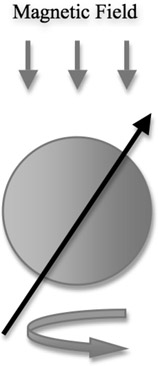
An atom (although a quantum-level object) can be described as a spinning top. Such a top will be precessing about its axis at an angle as shown in Figure 14.2. The frequency of the precession is an important factor and is described by the Larmor equation (Equation 14.1).
(14.1) |
|---|
where γ is the gyromagnetic ratio, f is the Larmor frequency, and B is the strength of the external magnetic field.
An atom in a magnetic field is aligned in the direction of the field. An RF pulse (to be introduced later) can be applied to change the orientation of the atom. If the magnetic field is pointing in the z-direction, the atom will be aligned in the z-direction. If a pulse of sufficient strength is applied, the atom can be oriented in the x-direction or y-direction or sometimes even in the z-direction, the direction opposite to its original.
If the RF pulse is removed, the atom returns to its original z-direction. During the process of moving from the xy-direction to the z-direction, the atom traces a spiral motion, described by the Bloch equations (Equation 14.2).
(14.2) |
|---|
The equations can be easily visualized by plotting them in 3D (Figure 14.3). At time t = 0, the value of Mz is zero. This is due to the fact that the atoms are oriented in the xy-plane and hence their net magnetization is also in the xy-plane and not in the z-direction. When the RF pulse is removed, the atoms begin to orient in the z-direction (their original direction before RF pulse). This change along the xy-plane is an exponential decay in amplitude change and sinusoidal in directional change. Thus, the net magnetization reduces over time exponentially while sinusoidally changing direction in the xy-plane. At t = infinity, the Mx and My reach 0 while Mz reaches the original value of M0.

Since a patient cannot be imaged for an infinite amount of time, in real applications, the atom will never recover its original magnetization completely.
The gyromagnetic ratio of a particle is the ratio of its magnetic dipole moment to its angular momentum. It is a constant for a given nuclei. The values of the gyromagnetic ratio for various nuclei are given in Table 14.1. When an object containing multiple materials (and hence different nuclei) is placed in a magnetic field of certain strength, the precessional frequency is directly proportional to the gyromagnetic ratios based on the Larmor equation. Hence, if we measure the precessional frequency, we can distinguish the various materials. For example, the gyromagnetic ratio is 42.58 MHz/T for a hydrogen nucleus while it is 10.71 MHz/T for a carbon nucleus. For a typical clinical MRI machine, the magnetic field strength (B) is 1.5T. Hence the precessional frequency of a hydrogen atom is 63.87 MHz and that of the carbon is 16.07 MHz.
TABLE 14.1: An abbreviated list of the nuclei of interest to NMR and MRI imaging and their gyromagnetic ratios.
|
Nuclei |
γ (MHz/T) |
|
H1 |
42.58 |
|
P31 |
17.25 |
|
Na23 |
11.27 |
|
C13 |
10.71 |
The second material property that is imaged is the proton density or spin density. It is the number of “mobile” hydrogen nuclei in a given volume of the sample. The higher the proton density, the larger the response of the sample in NMR or MRI imaging.
The response to NMR and MRI is not only dependent on the density of the hydrogen nucleus but also its configuration. A hydrogen nucleus connected to oxygen responds differently compared to the one connected to a carbon atom. Also, a tightly bound hydrogen atom does not produce any noticeable signal. The signal is generally produced by an unbound or free hydrogen nucleus. Thus, the hydrogen atom in tissue that is loosely bound produces a stronger signal. Bone on the other hand has hydrogen atoms that are strongly bound and hence produce a weaker signal.
Table 14.2 lists the proton density of common materials. It can be seen from the table that the proton density for bone is low compared to white matter. Thus, the bone responds poorly to the MRI signal. One exception in the table is the response of fat to the MRI signal. Although fat consists of a large number of protons, it responds poorly to the MRI signal. This is due to the long chain of molecules found in fat that immobilize hydrogen atoms.
TABLE 14.2: List of biological materials and their proton or spin density.
|
Biological material |
Proton or spin density |
|
Fat |
98 |
|
Grey matter |
94 |
|
White matter |
100 |
|
Bone |
1-10 |
|
Air |
< 1 |
14.3.3T1 and T2 Relaxation Times
There are two relaxation times that characterize the various regions in an object and can help distinguish them in an MRI image. They characterize the response of an atom in the Bloch equation.
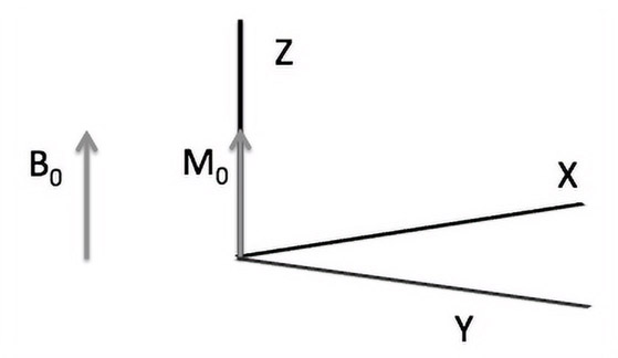
Consider the image shown in Figure 14.4. A strong magnetic field B0 is applied in the direction of the z-axis. This causes a net magnetization of M0 in the z-axis to increase from zero. The increase is initially rapid but then slows down. It is given by Equation 14.3 and graphically represented by Figure 14.5.
(14.3) |
|---|

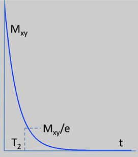
The time for the net magnetization to reach a value within e (i.e., ) is called the T1 relaxation time. Since T1 deals with both magnetization and demagnetization along the longitudinal direction (z-axis), T1 is also referred to as longitudinal relaxation time.
During an MRI image acquisition, in addition to the external magnetic field, an RF pulse is applied. This RF pulse disturbs the equilibrium and reduces Mz. The protons are not in isolation from other atoms but instead are bound tightly by a lattice. When the RF pulse is removed, the protons return to equilibrium, which causes a decrease in Mxy or transverse magnetization. This is accomplished by transferring energy to other atoms and molecules in the lattice. The time constant for the magnetization decay in the xy-axis is called T2 or the spin-lattice relaxation time. It is governed by Equation 14.4 and is graphically represented by Figure 14.6.
(14.4) |
|---|
T1 and T2 are independent of each other but T2 is generally smaller than or equal to T1. This is evident from Table 14.3, which lists T1 and T2 values for some common biological materials. The value of T1 and T2 are dependent on the strength of the external magnetic field (1.0T in this case).
TABLE 14.3: List of biological materials and their T1 and T2 values for field strength of 1.0 T.
|
Biological material |
T1 (ms) |
T2 (ms) |
|
Cerebrospinal fluid |
2160 |
160 |
|
Grey matter |
810 |
100 |
|
White matter |
680 |
90 |
|
Fat |
240 |
80 |
As discussed earlier, the presence of a strong magnetic field aligns the proton in the object in the direction of the magnetic field. The most interesting phenomenon happens when an RF pulse is applied to the object in the presence of the main magnetic field.
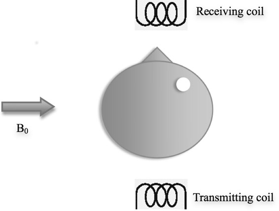
Due to the strong magnetic field (B0), the protons align themselves with it. They also precess at the Larmor frequency. This is the equilibrium state of the proton under the magnetic field. When an RF pulse is applied using the transmitting coil to the cartoon head (Figure 14.7), the proton orientation changes and in some cases it flips in the negative direction while precessing at the Larmor frequency. Due to the flip, the net magnetization is in the direction opposite to the direction of the main magnetic field. When the RF pulse is removed, the protons flip back to the positive direction and hence reach their equilibrium state. During this process, an electric current is induced in the receiving coil due to changing magnetic field. This based on Faraday’s law which was discussed previously. The signal obtained in the receiving coil is shown in Figure 14.8. The signal reduces in its intensity over time due to free induction decay (FID) and the time for the protons to reach their equilibrium state, or the “relaxed” state, is called the “relaxation time.”

The signal is a plot over time. This signal contains details of the frequencies of various protons in the object. The frequency distribution can be obtained by using Fourier transform.
14.5MRI Signal Detection or MRI Imaging
In this section, we will learn methods for obtaining images using MRI. The actual imaging process begins with selection of a section of the object being imaged and placing that section under a magnetic field in a process called slice selection. An MRI signal can only be achieved by changing the orientation of the proton under the magnetic field. This is achieved by applying an RF pulse in the other two orthogonal directions during phase and frequency encoding. All these activities need to be timed so that an MRI image can be obtained. This timing process is called the pulse sequence. We will discuss each of these in detail in the subsequent sections.
Slice selection is achieved by applying the magnetic field shown in Figure 14.5.1 on an object along one of the orthogonal directions in generally the z-direction or axial direction. Application of the magnetic field causes the protons in that section to orient themselves in the direction of the magnetic field and limits the imaging to this section. The slices that are not under the magnetic field are oriented randomly and hence will not be affected by the subsequent application of the magnetic field or RF pulses.

Phase encoding gradient is generally applied in the x-, y- or z- direction. Due to the application of slice selection gradient, the various protons are oriented in the z-direction (say). They will be spinning in phase with each other. By applying a gradient along the y-direction (say), the protons along a given y-location will spin with the same phase and the other y-locations will spin out of phase. Since every y-location can be identified using its phase, it can be concluded that the protons are encoded with reference to phase. The same argument can be extended if the phase encoding gradient is in the x-direction. If the MRI image has N pixel locations, the phase encoding gradient is chosen such that the phase shift between adjacent pixels is given by Equation 14.5. This ensures that two coordinates do not share the same phase.
(14.5) |
|---|
Frequency encoding gradient is applied in the x-, y- or z- direction. After the application of phase encoding gradient along the y-direction, all the protons along a given y-location will be precessing at the same phase. When a frequency encoding gradient is applied along the x-direction, protons for a given x-location will receive the same magnetic field. Hence these protons will precess at the same frequency. Thus, with the application of both phase and frequency encoding gradient, every x-, y- point in the object will have a unique phase and frequency.
A simple model (Figures 14.10 and 14.11) of an MRI will consist of:
•Main magnet
•Gradient magnet
•Radio-frequency coils
•Computer for processing the signal

FIGURE 14.10: Closed magnet MRI machine. Original image reprinted with permission from Siemens AG.
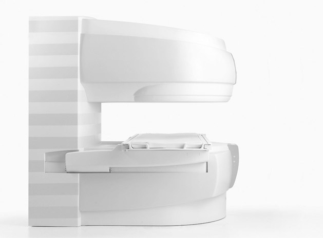
FIGURE 14.11: Open magnet MRI machine. Original image reprinted with permission from Siemens AG.
The main magnet generates a strong magnetic field. A typical MRI machine used for medical diagnosis is around 1.5T, which is 30,000 times stronger than the earth’s magnetic field.
The magnets could be permanent magnets, electromagnets or superconducting magnets. An important criterion for choosing a magnet is its ability to produce a uniform magnetic field. Permanent magnets are cheaper but the magnetic field is not uniform. Electromagnets can be manufactured to close tolerance, so that the magnetic field is uniform. They generate a lot of heat, which limits the magnetic field strength. Superconducting magnets are electromagnets that are cooled by superconducting fluids such as liquid nitrogen or helium. These magnets have a homogeneous magnetic field and high field strength but they are expensive to operate.
As described earlier, a uniform magnetic field cannot localize the various parts of the object. Hence gradient magnetic fields are used. Based on Faraday’s law, a magnetic field can be generated by the application of current to a coil, also known as gradient coils. Since gradient needs to be generated in all three directions, gradient coils are configured to generate fields in all three directions.
An RF coil is composed of loops of conducting materials such as copper. It generates a magnetic field with the passage of current. This process is called transmitting signal. Similarly, a rapidly changing magnetic field generates current in the coil which can be measured. This is accomplished using a receiving coil. In some cases, the same coil can transmit and receive signals. Such coils are called transceivers. An example of a brain imaging coil is shown in Figure 14.12. Specialized coils are created for different parts being imaged.

FIGURE 14.12: Head coil. Original image reprinted with permission from Siemens AG.
In Section 14.4, we discussed that the protons regain their orientation after the removal of the RF pulse. During this process, an FID signal (Figure 14.8) is induced in the coil. The FID signal is a plot over time of the change in the net-magnetization in the transverse plane. This signal contains various frequencies that can be obtained using Fourier transformation (Chapter 7). This signal is a 1D signal, as the originating signal is also 1D.
In Section 14.5, we also discussed that the three magnetic field gradients allow signal localization. The three magnetic fields are applied, and the signal obtained for each condition is read out. This 1D signal fills one horizontal line in the frequency space (Figure 14.13). By repeating the signal generation process for all conditions, the various horizontal lines can be filled.
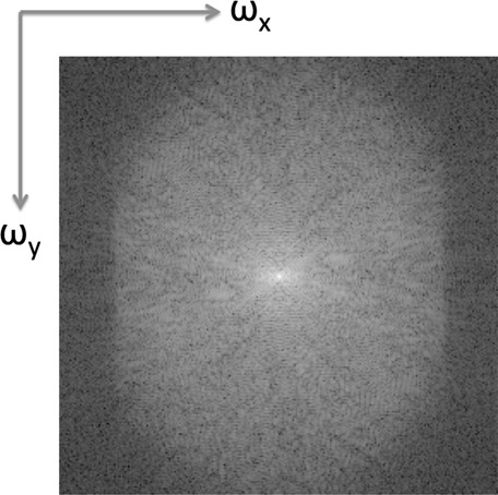
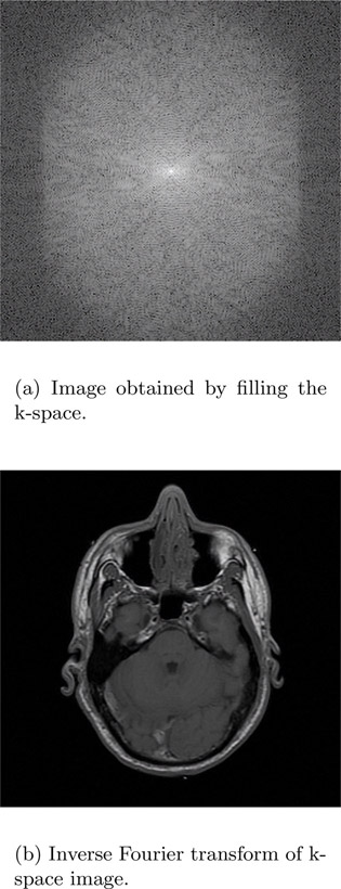
It can be proven that the image acquired in Figure 14.13 is the Fourier transform of the MRI image. A simple inverse Fourier transform can be used to obtain the MRI image (Figure 14.14). Figure 14.14(a) is the image obtained by filling the k-space and Figure 14.14(b) is obtained using the inverse Fourier transform of the first image.
14.7T1, T2 and Proton Density Image
A typical MRI image consists of T1, T2 and proton density weighted components. It is possible to obtain pure T1, T2 and a proton density weighted image but it is generally time consuming. Such images are used for discussion to emphasize the role each of these components plays in MRI imaging.
Figure 14.15(a) is a T1 weighted image (i.e., the pixel values are dependent on the T1 relaxation time). Similarly, Figure 14.15(b) and Figure 14.15(c) are T2 and proton density weighted images respectively.
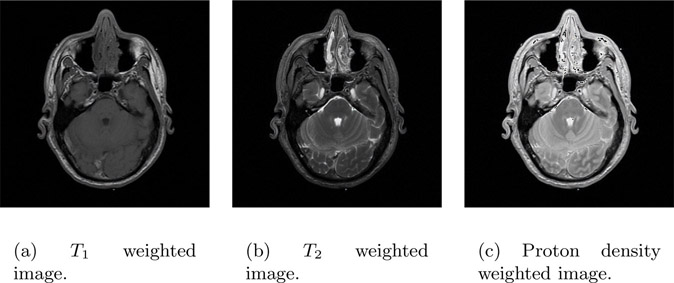
FIGURE 14.15: T1, T2 and proton density image. Courtesy of the Visible Human Project.
Bright pixels in a T1 weighted image correspond to fat, while the same pixels appear darker in a T2 weighted image and vice versa. A proton density image is useful in identifying the pathology of the object.
14.8MRI Modes or Pulse Sequence
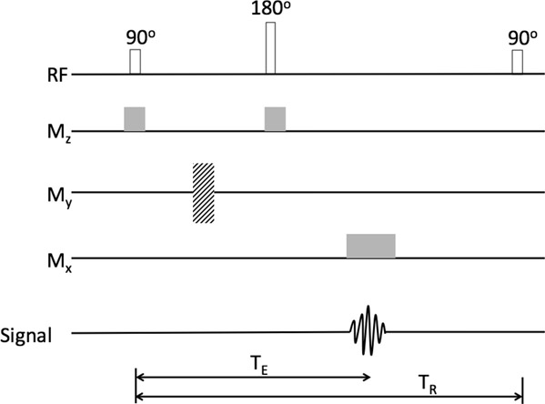
So far, we have learned about the various controls such as gradient magnitude along the three axes and the RF pulse that tilts the orientation of the protons. In this section, we will combine these four controls to produce images that are medically and scientifically useful. This process consists of performing different operations at different times and is generally shown using a pulse sequence diagram. In this diagram, each control receives its own row of operation. The time progresses to the right of each row. Some of these pulse sequences are discussed below. In each case, a certain set of operations or sequences is repeated at regular intervals called the repetition time or TR. TE is defined as the time between the start of the first RF pulse and the time to reach the peak of the echo (or output signal).
The spin echo pulse sequence (Figure 14.16) is one of the simplest and most commonly used pulse sequences. It consists of a 90-degree pulse followed by 180-degree pulse at TE/2. During both the pulses, the gradient magnitude along the z-axis is kept on. An echo is produced at time TE while the gradient along the x-axis is kept on so that localization information can be obtained. This process is repeated after every time to repeat (TR). The last 90-degree pulse in the figure is the start of the next sequence.
The inversion recovery pulse sequence (Figure 14.17) is similar to the spin echo sequence except for a 180-degree pulse applied before the 90-degree pulse.
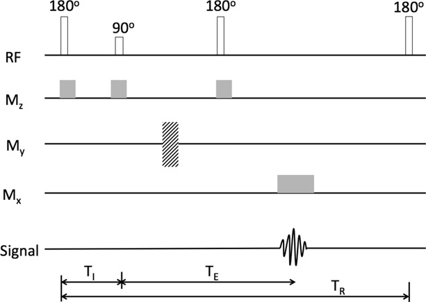
The 180-degree pulse causes the net-magnetization vector to be inverted along the z-axis. Since the inversion cannot be measured in planes other than xy-plane, a 90-degree pulse is applied. The time between the two pulses is called the inversion time or TI. The gradient magnetic field along the z-axis is kept on during both pulses. The gradient is applied while reading the echo, so that the localization information can be obtained. This process is repeated at regular intervals of TR. The last 180-degree pulse in the figure is the start of the next sequence.
Gradient echo imaging pulse sequence (Figure 14.18) consists of only one pulse of 90-degree and is one of the simplest pulse sequences. The flip angle could be any angle and 90-degree was chosen as one example. The slice selection gradient is kept on during the application of the 90-degree pulse. At the end of the pulse, a gradient magnetic field is applied along the y-axis. A negative gradient is applied along the x-axis at the same time. The x-axis gradient is then switched to positive gradient while the echo is read. Since there are fewer pulses and the gradient are switched on at consecutive intervals, it is one of the fastest imaging techniques. The last 90-degree pulse in the figure is the start of the next sequence.

By using various settings for TR and TE, it is possible to obtain images that are weighted for T1, T2 and proton density. A list of such parameters is shown in Table 14.4.
TABLE 14.4: TR and TE settings for various weighted images.
Weighted image |
TR |
TE |
T1 |
Short |
Short |
|
T2 |
Long |
Long |
|
Proton density |
Long |
Short |
Image formation in MRI is complex with interaction of various parameters such as homogeneity of the magnetic field, homogeneity of the applied RF signal, shielding of the MRI machine, presence of metal that can alter the magnetic field, etc. Any deviation from ideal conditions will result in an artifact that could either change the shape or the pixel intensity in the image. Some of these artifacts are easily identifiable. For example, a metal artifact leaves identifiable streaks or distortions. A few other artifacts are not easily identifiable. An example of an artifact that is not easily identifiable is the partial volume artifact.
These artifacts can be removed by creating close to ideal conditions. For example, to ensure that there are no metal artifacts, it is important that the patient does not have any implanted metal objects. Alternately, a different imaging modality such as CT or a modified form of MRI imaging can be used.
Artifacts are generally classified into two categories: patient related and machine related. The motion artifact and metal artifact are patient related while inhomogeneity and partial volume artifacts are machine related. An image may contain artifacts from both categories. There are many other artifacts. Interested readers must check the references in Section 14.1.
A motion artifact can be due to either motion of the patient or the motion of the organs in a patient. The organ motions occur due to cardiac cycle, blood flow, and breathing. In MRI facilities with poor shielding or design, moving large ferromagnetic objects such as automobiles, elevators, etc., can cause inhomogeneity in the magnetic field that in turn can cause motion artifacts.
Motion due to the cardiac cycle can be controlled by gating, a process of timing the image acquisition with the heart cycle. In some cases, simple breath holding can be used to compensate for the motion artifact.
Figure 14.19 is an example of a slice reconstructed with and without a motion artifact. The motion artifact in Figure 14.19(b) has resulted in significant degradation of the image quality, making clinical diagnosis difficult.

FIGURE 14.19: Effect of motion artifact on MRI reconstruction. Original images reprinted with permission from Dr. Essa Yacoub, University of Minnesota.
Ferromagnetic materials such as iron strongly affect the magnetic field, causing inhomogeneity. In Figure 14.20, the arrows in the two images indicate the direction of the magnetic field. In the left image, the magnetic field surrounds a non-metallic object such as tissue. The presence of the tissue does not change the homogeneity of the magnetic field. In the right image, a metal object is placed in the magnetic field. The magnetic field is distorted close to the object.
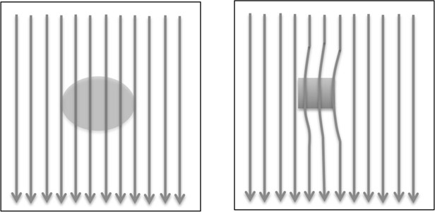
The reconstruction process assumes that the field is homogeneous. Thus, it assumes that all points with the same magnetic field strength will have the same Larmor frequency. This variation from ideality causes metal artifact.
The effect is more profound in the case of ferromagnetic materials such as iron, stainless steel, etc. It is less profound in metals such as titanium and other alloys. If MRI is the preferred modality for imaging a patient with metal implants, a low field-strength magnet can be used.
This artifact is similar in principle to the metal artifact. In the case of metal artifact, the inhomogeneity is caused by the presence of metallic objects. In the case of the inhomogeneity artifact, the magnetic field is not uniform due to a defect in the design or manufacture of the magnet.
The artifact can occur due to the main magnetic field (B0) or due to gradient magnetic field. In some cases, the main magnetic field may not be uniform across the patient and will change from center to periphery.
The artifact results in distortion depending on the variation of magnetic field across the patient. If the variations are minimal, the shading artifact results.
This artifact is caused by imaging using large voxel size, causing two nearby object intensities or pixel intensities to be averaged. This artifact generally affects long and thin objects as their intensity changes rapidly in the direction perpendicular to their long axis.
The artifact can be reduced by increasing the spatial resolution, which results in an increased number of voxels in the image and consequently longer acquisition time.
•MRI is a non-radiative high-resolution imaging technique.
•It works on Faraday’s law, Larmor frequency, and Bloch equation.
•It is based on physical principles such as T1 and T2 relaxation time, proton density, and gyromagnetic ratio.
•Atoms in a magnetic field are aligned in the direction of the magnetic field. An RF pulse can be applied to change their orientation. When the RF pulse is removed, the atoms reorient, and the current generated by this process can be measured. This is the basic principle of NMR.
•In MRI, the basic principle of NMR is used along with slice selection, phase encoding, and frequency encoding gradient to localize the atoms.
•An MRI machine consists of a main magnet, gradient magnets, an RF coil, and a computer for processing.
•The various parameters that control MRI image acquisition are diagrammatically represented as a pulse sequence diagram.
•MRI suffers from various artifacts. These artifacts can be classified as either patient related or machine related.
1.Calculate the Larmor frequency for all atoms listed in Table 14.1.
2.Explain the plot in Figure 14.3 using Equation 14.2.
3.If the plot in Figure 14.3 is viewed looking down in the z direction, the magnetic field path will appear as a circle. Why?
Solution: The values of Mx and My have cos and sin dependencies, similar to the parametric form of a circle.
4.Explain why T2 is generally smaller than or equal to T1.
5.Before k-space imaging was used, image reconstruction was achieved using a back-projection technique similar to CT. Write a report about this technique.
6.We discussed a few of the artifacts seen in MRI images. Identify two more artifacts and list their causes, symptoms and method to overcome these artifacts.
7.MRI is generally safe compared to CT. Yet it is important to take precautions during MRI imaging. List some of these precautions.