6.2.1Translation

Translation is the process of shifting the image along the various axes (x-, y- and z-axis). For a 2D image, we can perform translation along one or both axes independently. The transformation matrix for translation is defined as:

If we consider a pixel coordinate (x, y, 1) and perform the dot product with the translation matrix in Equation 6.1, we will obtain the pixel coordinate of the transformed matrix.

Thus every pixel in the transformed image is offset by t_x and t_y along x and y respectively. The value of t_x and t_y may be positive or negative.

The following code implements translation transformation. The image is read and converted in to a numpy array. The transformation matrix is created as an instance of the AffineTransform class. The translation value of (10, 4) is supplied as input to the AffineTransform class. If you need to visualize the value of the transformation matrix similar to one in Equation 6.1, you can print out the content of ‘transformation.params’. The transformation is supplied to the warp function which transform the input image img1 to the output image img2.

import numpy as np
import scipy.misc, math
from scipy.misc.pilutil import Image
from skimage.transform import AffineTransform, warp

img = Image.open(’../Figures/angiogram1.png’).convert(’L’)
img1 = scipy.misc.fromimage(img)

# translate by 10 pixels in x and 4 pixels in y
transformation = AffineTransform(translation=(10, 4))
img2 = warp(img1, transformation)
im4 = scipy.misc.toimage(img2)

im4.save(’../Figures/translate_output.png’)
im4.show()

The output of the translation is shown below. The image in Figure 6.1(a) is translated to produce the output image in Figure 6.1(b). The transformed image is translated by 10 pixels to the left and 4 pixels to the top with reference to the input image.

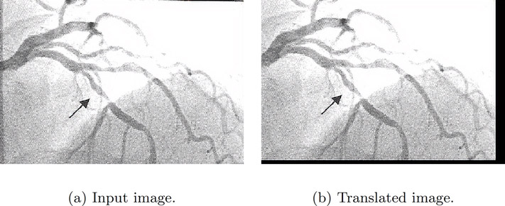
The missing pixel values on the right and bottom are given a value of 0 and hence the black pixels on the right and bottom edge. The warp function’s mode parameter can be used to modify this behavior. If the mode is, “constant” the value of cval parameter to the warp function will be used instead of a pixel value of 0. If the mode is, “mean”, “median”, “maximum”, or “minimum” a padding value equal to the mean, median, maximum or minimum along that vector will be used respectively. The readers are recommended to read the documentation for other options. The choice of the padding value affects the quality of the image and in some cases further computation.

6.2.2Rotation

Rotation is the process of changing the radial orientation of an image along the various axes with respect to a fixed point. The transformation matrix for a counter-clockwise rotation is defined as:

If we consider a pixel coordinate (x, y, 1) and perform the dot product with the rotation matrix in Equation 6.4, we will obtain the pixel coordinate for the rotated matrix.

The following code implements the rotation transformation. The image is read and converted into a numpy array. The transformation matrix is created as an instance of the AffineTransform class. The rotation value of 0.1 radians is supplied as input to the AffineTransform class. If you need to visualize the value of the transformation matrix similar to the one in Equation 6.4, you can print out the content of ‘transformation.params’. The transformation is supplied to the warp function, which transforms the input image img1 to the output image img2 using the transformation.

import numpy as np
import scipy.misc, math
from scipy.misc.pilutil import Image
from skimage.transform import AffineTransform, warp
img = Image.open(’../Figures/angiogram1.png’).convert(’L’)
img1 = scipy.misc.fromimage(img)

# rotation angle in radians
transformation = AffineTransform(rotation=0.1)
img2 = warp(img1, transformation)
im4 = scipy.misc.toimage(img2)
im4.save(’../Figures/rotate_output.png’)
im4.show()

The image in Figure 6.2(a) is rotated to produce the output image in Figure 6.2(b). The transformed image is rotated by 0.1 radians with reference to the input image. The missing pixel values on the left and bottom are given a value of 0 that can be modified by supplying appropriate values to the warp function’s mode parameter (as discussed in the previous section).

6.2.3Scaling

Scaling is a process of changing the distance (compression or elongation) between points in one or more axes. This change in distance causes the object in the image to appear larger or smaller than the original input. The scaling factor may be different across different axes. The transformation matrix for scaling is defined as:

If the value of k_x or k_y is less than 1, then the objects in the image will appear smaller ,and missing pixel values will be filled with 0 or based on the value of the warp parameter. If the value of k_x or k_y is greater than 1, then the objects in the image will appear larger. If the value of k_x and k_y are equal, the image is compressed or elongated by the same amount along both axes.

If we consider a pixel coordinate (x, y, 1) and perform the dot product with the scaling matrix in Equation 6.7, we will obtain the pixel coordinate for the scaled matrix.

The following code implements scaling transformation. The image is read and converted to a numpy array. The transformation matrix is created as an instance of the AffineTransform class. The scaling value of (0.5, 0.5) is supplied as input to the AffineTransform class corresponding to scaling along x and y axes. The transformation is supplied to the warp function, which transforms the input image img1 to the output image img2 using the transformation.

import numpy as np
import scipy.misc, math
from scipy.misc.pilutil import Image
from skimage.transform import AffineTransform, warp

img = Image.open(’../Figures/angiogram1.png’).convert(’L’)
img1 = scipy.misc.fromimage(img)

# scale by 1/2 on both x and y.
transformation = AffineTransform(scale=(0.5, 0.5))
img2 = warp(img1, transformation)
im4 = scipy.misc.toimage(img2)
im4.save(’../Figures/scale_output.png’)
im4.show()

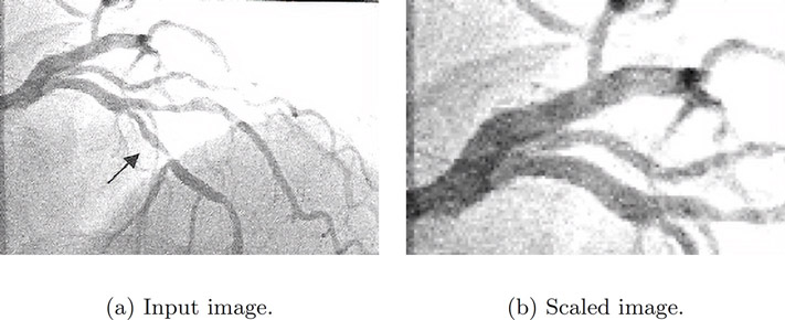
The image in Figure 6.3(a) is scaled to produce the output image in Figure 6.3(b). The image is scaled to 0.5 of its original size with reference to the input image along both axes.

6.2.4Interpolation

To understand the use of interpolation, we will first perform a thought experiment. Consider an image of size 2x2. If this image is scaled to four times its size in all linear dimensions, the new image will be of size 8x8. The original image has only 4 pixel values while the new image needs 64 pixel values. The question is: How can we fill 64 pixels with values given that there are only 4 pixel values? The answer is interpolation.

The various interpolation schemes available are:

1.Nearest-neighbor (order = 0)

2.Bi-linear (order = 1)

3.Bi-quadratic (order = 2)

4.Bi-cubic (order = 3)

5.Bi-quartic (order = 4)

6.Bi-quintic (order = 5)

The order number specified in parentheses is the number used by scikit-image. We will learn about the first 4 interpolation schemes. In all these schemes, the aim is to fill the missing pixel value.

In the nearest-neighbor interpolation,a the missing pixel value is determined based on its immediate neighbors. For a large scaling factor such as 2, we will assign 4 neighbors in the output image to the same pixel value as one of the pixels in the input image, thus making the output image appear pixelated. It is not recommended to use this interpolation even though it is the easiest to implement and also the fastest.

In the bi-linear interpolation, the missing pixel values are determined based on 2x2 pixels around the missing pixels. This results in a smoothed image with fewer artifacts compared to the nearest-neighbor interpolation. Since nearest-neighbor interpolation does not produce a good-quality image compared to other interpolation, it is recommended to use bi-linear at least. In scikit-image, bi-linear is the default interpolation.

In the bi-quadratic interpolation, the missing pixel values are determined based on 3x3 pixels around the missing pixels while in the bi-cubic interpolation, the missing pixel values are determined based on 4x4 pixels around the missing pixels. This results in a smoothed image with fewer artifacts compared to the bi-linear interpolation but at a higher computational cost.

The other two interpolations bi-quartic and bi-quintic, result in smoother interpolation but higher computational cost.

The following code demonstrates the effect of various interpolations. The image is read and converted to a numpy array. The transformation matrix is created as an instance of the AffineTransform class. The scaling value of (0.3, 0.3) is supplied as input to the AffineTransform class corresponding to scaling along x and y axes.

The transformation is then supplied to the warp functio,n which transforms the input image img1 to the output image img2 using the transformation with various interpolation schemes specified using the value for the parameter order. The transformed image for each of the interpolations is then stored.

import numpy as np
import scipy.misc, math
from scipy.misc.pilutil import Image
from skimage.transform import AffineTransform, warp

img = Image.open(’../Figures/angiogram1.png’).convert(’L’)
img1 = scipy.misc.fromimage(img)

transformation = AffineTransform(scale=(0.3, 0.3))

# nearest neighbor order = 0
img2 = warp(img1, transformation, order=0)
im4 = scipy.misc.toimage(img2)
im4.save(’../Figures/interpolate_nn_output.png’)
im4.show()

# bi-linear order = 1
img2 = warp(img1, transformation, order=1) # default
im4 = scipy.misc.toimage(img2)
im4.save(’../Figures/interpolate_bilinear_output.png’)
im4.show()

#bi-quadratic order = 2
img2 = warp(img1, transformation, order=2)
im4 = scipy.misc.toimage(img2)
im4.save(’../Figures/interpolate_biquadratic_output.png’)
im4.show()

#bi-cubic order = 3
img2 = warp(img1, transformation, order=3)
im4 = scipy.misc.toimage(img2)
im4.save(’../Figures/interpolate_bicubic_output.png’)
im4.show()

The image in Figure 6.4(a) is scaled to produce all the other images. The image in Figure 6.4(b) used nearest neighbor interpolation, the image in Figure 6.4(c) used bi-linear interpolation, the image in Figure 6.4(d) used bi-quadratic interpolation and the image in Figure 6.4(e) used bi-cubic interpolation. As can be seen in the image, the nearest-neighbor performed poorly as it exhibits pixelation compared to all other methods. The quality of the image for all other cases are similar but the cost increases significantly for all other methods.