Neural networks has taken the world by storm in the last decade. However, the work has been ongoing since the 1940s. Some of the initial work was in modeling the behavior of a biological neuron mathematically. Frank Rosenblat in 1958 built a machine that showed an ability to learn based on the mathematical notion of a neuron. The process of building neural networks were further refined over the next 4 decades. One of the most important papers that allowed training arbitrarily complex networks appeared in 1986 in a work by David E. Rumelhart, Geoffrey Hinton, and Ronald J. Williams [RHW86]. This paper re-introduced the back-propagation algorithm that is the workhorse of the neural network as used today. In the last 2 decades, due to the availability of cheaper storage and compute, large networks have been built that solve significant practical problems. This has made the neural network and its cousins such as the convolution neural network, recurrent neural network, etc., household names.
In this chapter, we will begin the discussion with the mathematics behind neural networks, which includes forward and back-propagation. We will then discuss the visualization of a neural network. Finally, we will discuss building a neural network using Keras, a Python module for machine learning and deep learning.
Interested readers are recommended to follow the discussions in the following sources: [Dom15], [MTH], [GBC16], [Gro17].
A neural network is a non-linear function with many parameters. The simplest curve is a line with two parameters: slope and intercept. A neural network has many more parameters, typically in the order of 10,000 or more and sometimes millions. These parameters can be determined by the process of optimizing a loss function that defines the goodness of fit.
We will begin the discussion of the mathematics of a neural network by fitting lines and planes. We can then extend it to any arbitrary curve.
The equation of a line is defined as
(11.1) |
|---|
where x is the independent variable, y1 is the dependent variable, W is the slope of the line and b is the intercept. In the world of machine learning, W is called the weight and b is the bias.
If the independent variable x is a scalar, then Equation 11.1 is a line, W is scalar and b is a scalar. However, if x is a vector, then Equation 11.1 is a plane, W is a matrix and b is a vector. If x is very large, Equation 11.1 is called a hyper-plane. Equation 11.1 is a linear equation and the best model that can ever be created using it would be a linear model as well.
In order to create non-linear models in a neural network, we add a non-linearity to this linear model. We will discuss one such non-linearity called sigmoid. In practice however, other non-linearities such as tanh, rectified linear unit (RELU), and leaky RELU are also used.
The equation of a sigmoid function is
(11.2) |
|---|
When x is a large number, the value of y asymptotically reaches 1 (11.1), while for small values of x, the value of y asymptotically reaches 0. In the region along the x-axis between −1 and +1 approximately, the curve is linear and is non-linear everywhere else.

If the y1 from 11.1 is passed through a sigmoid function, we will obtain a new y1,
(11.3) |
|---|
where W1 is the weight of the first layer and b1 is the bias of the first layer. The new y1 in Equation 11.3 is a non-linear curve. The equation can be rewritten as,
(11.4) |
|---|
In a simple neural network here, we will add another layer (i.e., another set of W and b) to which we will pass the y1 obtained from Equation 11.4.
(11.5) |
|---|
where W2 is the weight of the second layer and b2 is the bias of the second layer.
If we substitute 11.4 in 11.5, we obtain,
(11.6) |
|---|
We can repeat this process by adding more layers and create a complex non-linear curve. However, for clarity sake, we will limit ourselves to 2 layers.
In Equation 11.6, there are 4 parameters namely, W1, b1, W2, and b2. If x is a vector, then W1 and W2 are matrices and b1 and b2 are vectors. The aim of a neural network is to determine the value inside these matrices and vectors.
The value of the 4 parameters can be determined using the process of back-propagation. In this process, we begin by assuming an initial value for the parameters. They can be assigned a value of 0 or some random value could be used.
We will then determine the initial value of y using Equation 11.6. We will denote this value as . The actual value y and the predicted value will not be equal. Hence there will be an error between them. We will call this error “loss.”
(11.7) |
|---|
Our aim is to minimize this loss by finding the correct value for the parameters of Equation 11.6.
Using the current value of the parameter, its new value iteratively can be calculated using,
(11.8) |
|---|
where W is a parameter and L is the loss function. This equation is generally called an ‘update equation’.
To simplify the calculation of partial derivatives such as , we will derive them in parts and assemble them using chain rule.
We will begin by calculating using Equation 11.7
(11.9) |
|---|
Then we will calculate using the chain rule,
(11.10) |
|---|
If we substitute from Equation 11.5 and from Equation 11.9, we obtain,
(11.11) |
|---|
The partial derivative can then be used to update the value of W2 using the existing value of W2 with the help of the update equation. A similar calculation (left as an exercise to the reader) can be shown for b2 as well.
Next we will calculate the new value of W1,
(11.12) |
|---|
which can be computed using Equations 11.9, 11.5 and 11.4 respectively. Thus,
(11.13) |
|---|
which can be simplified to
(11.14) |
|---|
The new value of W1 can be calculated using the update Equation 11.8. A similar calculation (left as an exercise to the reader) can be shown for b1 as well.
For every input data point or a batch of data points, we perform forward propagation, determine the loss, and then back-propagate to update the parameters (weights and biases) using the update equation. This process is repeated with all the available data.
In summary, the process of back-propagation finds the partial derivatives of the parameters of a neural network system and uses the update equation to find a better value for the parameters by minimizing the loss.
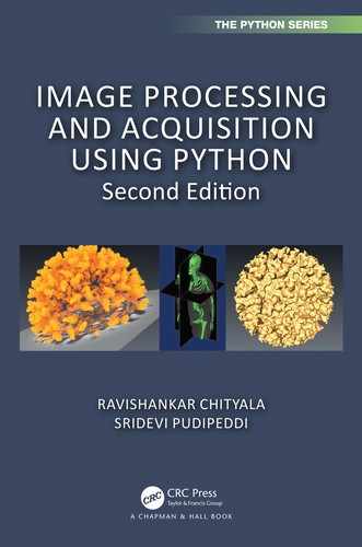
Typically, a neural network is represented as shown in Figure 11.2. The left layer is called the input layer, the middle is called the hidden layer, and the right is called the output layer.
A node (filled circle) in a given layer is connected to all the nodes in the next layer but is not connected to any nodes in that layer. In Figure 11.2, arrows are only drawn to originate from an input layer to the first node in the hidden layer. For clarity sake, the lines ending on other nodes are omitted. The values at each of the input nodes is multiplied with the weights in the line between the nodes. The weighted inputs are then added in the node in the hidden layer and passed through the sigmoid function or any other non-linearity. The output of the sigmoid function is then weighted in the next layer and the sum of all those weights will be the output of the output layer ().
If there are n nodes in the input layer and m nodes in the hidden layer, then the number of edges connecting from the input to hiddenlayer will be n*m. This can be represented as a matrix of size [n, m]. Then the operation described in the previous paragraph will be a dot product between the input x and the matrix followed by application of the sigmoid function described in Equation 11.4. This matrix is the W1 we have previously described.
If there are m nodes in the hidden layer and k nodes in the output layer, then the number of edges connecting from hidden to output will be m*k. This can be represented as a matrix of size [m, k] and is the matrix W2 we have previously described.
During the forward propagation, a value of x is used as an input to begin the compute that is propagated from the input side to the output. The loss is calculated by comparing the predicted value and the actual. The gradients are then computed in reverse from the output layer toward the input and the parameters (weights and biases) are updated by back-propagation.
In this discussion, we assumed that y is a continuous function and its value is a real number. This class of problem is called a regression problem. An example of such a problem is the prediction of price of an item based on images.
11.5Neural Network for Classification Problems
The other class of problem is the classification problem where the dependent variable y takes discrete values. An example of such a problem is identifying a specific type of lung cancer given an image. There are two major types: small cell lung cancer (SCLC) and non-small cell lung cancer (NSCLC).
In a classification problem, we aim to draw a boundary between two classes of points as shown in Figure 11.4. The two classes of points in the image are the circles and the plusses. A linear boundary (such as a line or plane) that has the lowest error cannot be drawn between these two sets of points. A neural network can be used to draw a non-linear boundary.

FIGURE 11.3: Graphical representation of a neural network as weight matrices.

FIGURE 11.4: The neural network for the classification problem draws a non-linear boundary between two classes of points.
One of the common loss functions for the classification problem is the cross entropy loss. It is defined as
(11.15) |
|---|
where y is the actual value and is the predicted value.
Since the loss function is different compared to the regression problem, the derivatives such as would yield a different equation compared to the one derived for the regression problem. However the approach remains the same.
11.6Neural Network Example Code
The current crop of popular deep learning packages such as Tensorflow [ABC+16], Keras [C+20], etc., require the programmer to define the forward propagation while the back-propagation is handled by the package.
In the example below, we define a neural network to solve the problem of identifying handwritten digits from MNIST dataset [LCB10], a popular image dataset for benchmarking machine learning and deep learning applications. Figure 11.5 shows a few representative images from the MNIST dataset. Each image is 28 pixels by 28 pixels in size. The total number of pixels = 28*28 = 784. The images contain a single hand-drawn digit. As can be seen in the image, two numbers may not look the same in two different images. The task is to identify the digit in the image, given the image itself. The image is the input and the output is one of the 10 classes (number between 0 and 9).
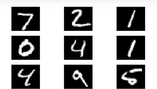
FIGURE 11.5: Some sample data from the MNIST dataset [LCB10].
We begin by importing all the necessary modules in Keras, specifically the Sequential model and Dense layer. The Sequential model allows defining a set of layers. In the mathematical discussion, we defined 2 layers. In Keras, these layers can be defined using the Dense layers class. A stack of these layers constitutes a Sequential layer.
We load the MNIST dataset using the convenient functionality (keras.datasets.mnist.load_data) available in Keras. This loads both the training data as well as testing data. The number of images in the training dataset is 60,000 and the number of images in the testing dataset is 10,000. Each image is stored as a 784-pixel-long vector with 8-bit precision (i.e., pixel values are between 0 and 255). The corresponding y for each image is a single number corresponding to the digit in that image.
We then normalize the image by dividing each pixel value by 255 and subtracting 0.5. Hence the normalized image will have pixel values between −0.5 and +0.5.
The model is built by passing 3 Dense layers to the Sequential class. The first layer has 64 nodes, the second layer has 64 nodes. The first 2 layers use the Rectified Linear Unit (RELU) activation function for non-linearity. The last layer produces a vector of length 10. This vector is passed through a softmax function (Equation 11.16). The output of a softmax function is a probability distribution as each of the values corresponds to the probability of a given digit and also the sum of all the values in the vector equates to 1. Once we obtain this vector, determining the corresponding digit can be accomplished by finding the position in the vector with the highest probability value.
(11.16) |
|---|
We will pass the model through an optimization process by calling the fit function. We run the model through 5 epochs, where each epoch is defined as visiting all images in the training dataset. Typically we feed a batch of images for training instead of one image at a time. In the example, we use a batch of 32, which implies in each training a random batch of 32 images and the corresponding labels are passed.
import numpy as npfrom keras.models import Sequentialfrom keras.layers import Densefrom keras.utils import to_categoricalfrom keras.datasets import mnist# Fetch the train and test data.(x_train, y_train), (x_test, y_test) = mnist.load_data()# Normalize the image so that all pixel values# are between -0.5 and +0.5.x_train = (x_train / 255) - 0.5x_test = (x_test / 255) - 0.5# Reshape the train and test images to size 784 long vector.x_train = x_train.reshape((-1, 784))x_test = x_test.reshape((-1, 784))# Define the neural network model with 2 hidden layer# of size 64 nodes each.model = Sequential([Dense(64, activation=’relu’, input_shape=(784,)),Dense(64, activation=’relu’),Dense(10, activation=’softmax’),])# Compile the model using Adam optimizer and use# the cross entropy loss.model.compile(optimizer=’adam’,loss=’categorical_crossentropy’,metrics=[’accuracy’])# Train the model.model.fit(x_train, to_categorical(y_train), epochs=5, batch_size=32)
The output contains the result of training 5 epochs. As can be seen the value of cross entropy loss decreases as the training progresses. It started at 0.3501 and finally ended at 0.0975. Similarly, the accuracy increased as the training progressed from 0.8946 to 0.9697.
Epoch 1/560000/60000 [===] - 3s 58us/step - loss: 0.3501 - accuracy:0.8946Epoch 2/560000/60000 [===] - 3s 56us/step - loss: 0.1790 - accuracy:0.9457Epoch 3/560000/60000 [===] - 3s 55us/step - loss: 0.1357 - accuracy:0.9576Epoch 4/560000/60000 [===] - 3s 55us/step - loss: 0.1129 - accuracy:0.9649Epoch 5/560000/60000 [===] - 3s 57us/step - loss: 0.0975 - accuracy:0.9697
Interested readers must consult the Keras documentation for more details.
•Neural networks are universal function approximators. In training a neural network, we fit a non-linear curve using available data.
•To obtain non-linearity in a neural network, we combine a linear function with non-linear functions such as sigmoid, RELU, etc.
•The parameters of the non-linear curve are learnt through the process of back-propagation.
•Neural networks can be used for both regression and classification problems.
1.You are given a neuron that performs addition of y = x1*w1+x2*w2, where x1 and x2 are the inputs and w1 and w2 are weights. Write the back-propagation equation for it. Also write the update equation for w1 and w2.
2.In a neural network, we combine linear function Wx + b with a non-linear function. We stack these layers together to produce an arbitrarily complex non-linear function. What would happen if we do not use a non-linear function but still stack layers? What kind of curve can we build?
3.Why is sigmoid no longer popular as an activation function? Conduct research on this topic.