
Chapter 21
Structured Query Language (SQL)
This chapter introduces the reader to Structured QueryLanguage (SQL), which is a standard computer language foraccessing and manipulating databases. It is used by the useras a means of communication to the database managementsystem (DBMS). SQL commands consist of English-likestatements, which are used to query, insert, update, anddelete data. The chapter starts by describing the role andcharacteristics of SQL in a DBMS environment and how itevolved as a database language. The rest of the discussionis focussed on some of the most important and commonlyused SQL commands and queries.
After reading this chapter, you will be able to understand:
Structured query language, which is used to define and manipulate data stored in a database
Concepts such as data definition language and data manipulation language
DDL commands that are used to create or delete database objects such as tables and indexes
DML commands, which operate on the data in a database
Querying multiple tables that are used to maintain large databases
SELECT statements, which can be used to break down a complex query into a series of logical steps
21.1 INTRODUCTION
In the previous chapter, we investigated the database, tables and records, and many such database-related issues. Database is a collection of interrelated information in a structured way, so that information can be easily retrieved, managed, and updated. Typically, a database is organized into tables, where each table is similar to a spreadsheet. A table has a set of columns (fields), each of which identifies some particular kind of information, and a set of rows (records) in which data are stored. There are lots of database management software available in the market such as Oracle and Sybase. Each database management system (DBMS) has its own programming language, using which a user can “talk” to the database and extract useful information. However, it would be difficult for a normal user to learn all these vendor-specific languages. For a user to write programs that interact with the databases easily, there has to be a way such that the user could use the same method to obtain information from all these databases. Hence, a new language was developed to overcome this barrier and enable data to be retrieved from any database software. This query language is called structured query language (abbreviated SQL, pronounced as “see kwell” or “ess queue ell”).
THINGS TO REMEMBER
SQL
SQL eases the burden of programmers and other users, as they need not know how or where data are stored. They just have to specify what is required and how the specified data sets should be presented (for example, conditions or additional computations such as sum and average). It is just like querying in simple English, which allows the user to specify how the human conceptualizes the query in mind. Translating certain complex queries into SQL statements may be difficult and the constructs may not be powerful enough to define certain requirements.
SQL is an international standard (both American National Standards Institute, ANSI, and International Standards Organization, ISO, have standardized it) for defining and manipulating data sets from a database. Nowadays, almost all industrial-strength database vendors support SQL. Each vendor may have its own version of SQL implementing features, unique to that software, but all SQL-enabled databases support a common standardized subset of SQL. Using SQL, one can retrieve data from a database, create database and database objects, add data, modify existing data, and perform various other functions.
Note: SQL provides a convenient method to create and manipulate databases. Moreover, SQL makes developing applications relatively easier.
21.1.1 Communicating with Database Using SQL
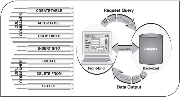
SQL is simply a database language and by itself does not constitute a DBMS. It is just a medium of communicating to the DBMS what the user wants it to do. SQL is sometimes referred to as a non-procedural database language. It implies that the SQL statements describe what data are to be retrieved, rather than specifying how to find the data. The DBMS will take care of locating the requested data from the database. Generally, corporate databases are stored on several different computers. In such situations, the non-procedural nature of SQL makes flexible, ad-hoc queries for data retrieval. Users can construct and execute an SQL query, analyse the retrieved data, and change the query (if needed), all in a spontaneous manner (Figure 21.1).
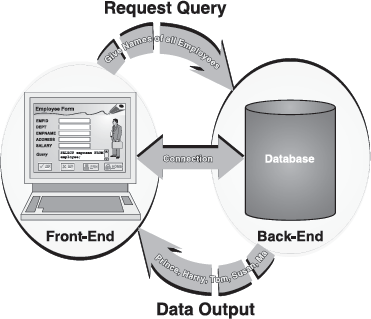
Figure 21.1 Communicating with Datavbase Using SQL
As discussed previously, SQL is used for communication with databases. The communicating parties are typically a front-end and a back-end. The front-end sends an SQL statement (containing instructions to create, read, change, or delete data) across a connection to a back-end that holds the data. Usually, the front-end includes an interface to users, such as Visual Basic or C++, with a “form” to gather data and buttons to carry out tasks. It may also contain fixed SQL statements or use code to create SQL statements on the fly using the data provided by the user. Back-ends are DBMSs such as Oracle and Sybase. They can accept an SQL statement and return a result. Usually, the back-end has two parts, the actual store of data and a database engine. The engine carries out the SQL statement and typically has a code that can search, read, write, index, and execute the actual interaction with the information. The front-end and back-end are linked via a “connection,” which provides a way to get the SQL statement to the back-end and then to return results to the front-end. A common connection used nowadays is ODBC (Open Database Connectivity).
By analogy, if the front- and back-end are like telephone handsets, then the connection is like a telephone connection over which a spoken language travels, although the language itself is free. To start a call, we first establish a connection by dialling the other party number and waits for the exchange to connect the correct wires. Then we can begin the conversation using a language like English across the connection. In the same way, a connection between front- and back-end software is created, and SQL statements are used to communicate across that connection.
21.1.2 Characteristics of SQL
SQL, tested and true over many years, is the standard way to communicate with a database. It is almost universally understood by both front-ends and back-ends. The amalgamation of SQL language and relational database management systems (RDBMSs) is one of the most cherished achievements of the computer industry. Over the last few decades, DBMS has grown tremendously and this alone is worth tens of billions of dollars, and SQL stands today as the standard database language. From its obscure beginning as an IBM research project, SQL has come of age as an important computer technology and a powerful market force. Some of the characteristics of SQL are briefed below.
- Standard Independent Language: The universal rules of the SQL have been established by ANSI and ISO. Therefore, the SQL is an open language, implying it is not owned or controlled by any single company. Today, SQL is offered by all the leading DBMS vendors. SQL is not just for a particular product; it works with Oracle, Microsoft SQL Server, and Sybase, just to name a few. Each vendor may have their proprietary extensions to SQL, but the basics of SQL are almost identical across all the database vendors. It means, regardless of the DBMS, the result of an SQL query will be the same. This vendor independence has enabled programmers to develop truly independent database applications.
- Cross-Platform Abilities: One of the biggest hardships of using a programming language to access database is that it seldom produces a “true” cross-platform application. SQL may be relatively new to some of the most popular programming languages like COBOL or C, but it has been in use on different hardware platforms for years. In most cases, the same SQL statement can be used on a desktop, a server, or a mainframe. An SQL-enabled database and the programs that use it can be moved from one DBMS to another vendor's DBMS with minimal (or no) conversion effort.
- Easy to Learn and Use: SQL statements resemble simple English sentences, making SQL easy to learn and understand. SQL has been created such that it is intuitive, simple, non-procedural (one need not specify step-by-step instructions to execute certain actions), and maps human's cognitive model. Being non-procedural in nature, the user just has to type a single SQL declaration and hand it to the DBMS. The DBMS then executes internal code (hidden from the user) and returns a set, which is a group of data that is logically defined.
- Less Programming: SQL allows extraction, manipulation, and organization of data with less programming as compared to traditional methods. SQL allows for record sets that are more complex to be created but requires less coding. It also allows tables to be joined together in ways that are not easily accomplished in other programming languages. Since SQL is a text-based programming language (that is, no executables are created for SQL-only programs), the SQL statement can also be constructed at run-time to give programs amazing flexibility. Furthermore, SQL can be used from within most programming languages. Whether you code in C++ or Java, SQL is the method of choice for accessing data.
- Universality: An alternative to using SQL statements is to write code in a procedural language like C++. The problem with this approach is that you are then closely tied to the procedural language, the metadata, and the specific DBMS. If there is a change in the structure of the tables, the code must be changed. If a new DBMS is installed, most of the codes must be revised to mesh with the new DBMS system of pointers, record set definitions, and so on. However, by using SQL statements, almost all changes are handled by the DBMS, behind the scenes from the programmer.
- Scaling: Many applications are developed for desktop environments. As they grow, a number of problems become apparent with these systems. For example, database software designed for the desktop generally fails when numerous people try to use the data at the same time. Therefore, organization has to move from desktop systems to a more robust DBMS. Almost all these heavy-duty DBMS rely on SQL as the main form of communication to scale well.
- Speed: Over the last 10 years, SQL data engines have been the focus of an intense effort to improve performance. The intense competition among database vendors has resulted in faster, more robust DBMSs that work at lower costs per transaction. Although SQL itself does not alleviate speed problems, the implementation of faster DBMS does, and those faster DBMSs require communications in SQL.
- Cost Effective: It is more expensive to run a server-centric DBMS (that only speaks SQL) than it is to use a desktop system (which does not necessarily need to use SQL). First, the software is more expensive. Second, in most cases, operating systems that are more expensive are needed to run in order to support the DBMS. Third, the operating system is required to be tuned differently to optimize for a DBMS than for other applications. Last, personnel with more expensive qualifications are engaged. However, the price of hardware and software is frequently the smallest item in an IT budget. As the data centre grows, at some point, the reliability, performance, and standardization benefits of a DBMS that uses SQL outweigh the cost.
Nowadays, most commercial DBMSs allow SQL to be used in two different ways. First, SQL commands can be typed at the command line directly. The DBMS interprets and processes the commands instantly and displays the retrieved result rows (if any). This method is known as interactive SQL. The second method is called embedded SQL (or programmatic SQL), where SQL statements are embedded in a host language like COBOL or C. The host language provides more flexibility in SQL because SQL does not have any statements or constructs that allow a program to “branch” or “loop.” The host language provides the necessary looping and branching structures, and the interface with the user, while SQL provides the statement to communicate with the DBMS. As a language, SQL plays many different roles:
- It is an interactive language because the user gains access to the data by issuing the desired query. This provides a convenient, easy-to-use tool for ad-hoc database queries.
- It is a database programming language because SQL commands can easily be embedded into application programs to access the data from a database.
- It is a database administration language because the database administrator uses SQL to define the database structure and control access to the stored data.
- It is a client/server language because it can be used to access remote (over a network) databases.
- It is a distributed database language because SQL helps in distribution of data across many connected computer systems.
SQL is a comprehensive language for controlling and interacting with a DBMS. However, it is not a program or a development environment such as Visual Basic or C++. There is no front-end built into SQL, neither does SQL have a back-end. There are no tools intrinsic to the language that can actually store data. SQL is only a standard means of communicating with software products that can hold data. As discussed previously, SQL is non-procedural in nature. Consequently, it can execute only one command at a time. SQL is not a particularly structured language, especially when compared to highly structured languages such as C or Java. SQL does not provide decision-making constructs such as IF-THEN-ELSE, DO-WHILE, and so on. Therefore, the user cannot use the results of an action to perform another action. In addition, SQL does not provide any error-handling procedures. Hence, to get the best out of SQL, it is embedded into other languages, such as COBOL or C, to extend that language for use in database access. Besides, SQL itself is not a DBMS, nor a stand-alone product. SQL cannot be bought “off-the-shelf.” Instead, it is an integral part of a DBMS, and it acts as a tool for communicating with the DBMS. SQL has emerged as the standard language for using relational databases. Its overwhelming features make it the most popular and powerful database language available today.
21.1.3 Brief History of SQL
The history of SQL began in an IBM laboratory in San Jose, California, where SQL was developed in the 1970s. The publication of Dr Edgar Codd's rules resulted in a considerable amount of relational database research done in the early 1970s. By 1974, the IBM had surfaced with a prototype of a relational database called System/R. Although the System/R project ended in 1979, two significant accomplishments were accredited to that project. The relational data model's viability was sufficiently proven to the world and the project included significant work on a database query language. By the end of the System/R project, IBM had implemented a language that enabled the programmers to define, query, or manipulate database with simple English-like statements. This language was named as the structured English query language (SEQUEL). The name later was shortened to structured query language (SQL). Today, many users still pronounce the abbreviation as “sequel” because of these early roots.
THINGS TO REMEMBER
History of SQL
A group of engineers watching the System/R project realized relational database's potential and formed a company named Relational Software Inc. In 1979, they produced the first commercially available RDBMS (called Oracle) and implemented SQL as its query language. Since then, many RDBMSs have come to market—all supporting SQL as their primary language.
SQL Standards: A database language standard specifies the semantics of various components of a DBMS. It defines the structures and operations of a data model implemented by the DBMS, as well as other components that support data definition, data access, security, programming language interface, and data administration. The SQL standard specifies data definition, data manipulation, and other associated facilities of a DBMS that supports the relational data model.
As discussed previously, SQL is a standard, open language without corporate ownership. The commercial acceptance of SQL was begun by the formation of SQL Standards Committees by the ANSI and the ISO. ANSI standardized SQL in 1986 and ISO standardized it in 1987. In 1989, a revised standard known commonly as SQL89 (also called SQL1) was published. However, due to conflicting interests from commercial vendors, much of the SQL89 standard was intentionally left incomplete, and many features were labelled implementer defined. In order to strengthen the standard, the ANSI committee revised the previous standard in 1992, and SQL92 (also called SQL2) was conceived. Afterwards, various SQL standards were released including SQL99, SQL2003, and SQL2006. The latest standard is SQL2008, which is the sixth standard of SQL (Table 21.1).
Table 21.1 SQL Standards
| Year | Name | Description |
|---|---|---|
| 1986 | SQL86 | First published by ANSI in 1986 and ratified by ISO in 1987 |
| 1989 | SQL89 | Some minor revision |
| 1992 | SQL92 | Major revisions were made |
| 1999 | SQL99 | Added regular expression matching, recursive queries, triggers, non-scalar types, some object-oriented features |
| 2003 | SQL2003 | Introduced XML-related features, standardized sequences, and columns with auto-generated values |
| 2006 | SQL2006 | Defined ways of importing and storing XML data in an SQL database, manipulating it within the database and publishing both XML and conventional SQL data in XML form |
| 2008 | SQL2008 | Added INSTEAD OF triggers and the TRUNCATE statement |
21.2 GETTING STARTED WITH SQL
Previously, we defined SQL as a query language that allows access to data residing in a DBMS. Users execute queries to extract information from the database using criteria that are defined by the user. The main objectives of SQL queries are:
- Defining database and its objects such as tables, attributes, data type, relational keys (primary key, foreign key, etc.), and indexes.
- Defining data access controls on tables through Grants and Views.
- Altering, dropping, and replacing the tables and others database objects.
- Inserting, updating, and deleting data in the tables.
- Performing queries that involve table joins; various types of conditions and nested queries.
The first three objectives are generally called data definition language (DDL) since they involve definition and management of the basic structure of the database. DDL commands are used primarily by database administrators during the set up and removal phases of a database project. The last two objectives are referred as data manipulation language (DML). DML is used to retrieve, insert, and modify database information and DML commands will be used by all database users during the routine operation of the database.
21.2.1 Data Types
SQL is considered a strongly typed language. This means that any piece of data represented by a table's field has an associated data type, that is, a set of rules describing a specific set of information, including the allowed range and operations and how information is stored. When the table is defined, every field in it is assigned a data type such as character, numeric, and so on. The type of a data value both defines and constraints the kinds of operations, which may be performed on it. SQL has numerous data types, such as Char, Numeric, and Date. Some of the most commonly used SQL data types are listed in Table 21.2.
Table 21.2 Common SQL Data Types
| Data Type | Description |
|---|---|
| Char(Size) | It defines a fixed Size-length character string (can contain letters, numbers, and special characters), where Size can be a maximum of 255 |
| Varchar(Size) | It defines a variable-length character string (can contain letters, numbers, and special characters) of up to Size characters |
| Integer | It defines an integer-only data type (usually a 32-bit signed integer) |
| Numeric(S,D) or Decimal(S,D) | It holds numbers with fractions. The maximum numbers of digits are specified in S. The maximum number of digits to the right of the decimal is specified in D |
| Date | This data type is used to store date. By default, the format is YYYY-MM-DD |
| Time | This data type is used to store time. By default, the format is HH:MM:SS |
| Boolean | This data type accepts a single value that can be true or false |
21.2.2 SQL Syntax
SQL input consists of a sequence of commands, and each command is composed of a sequence of tokens, terminated by a semicolon (“;”), although it is not essential. The end of the input stream also terminates a command. The validity of tokens depends on the syntax of the particular command. A token can be a keyword, an identifier, a literal (or constant), or a special character symbol. Generally, tokens are separated by white space (space, tab, or new line). For example, the following is (syntactically) a valid SQL input:
SELECT * FROM EMPLOYEE;
UPDATE EMPLOYEE SET Salary = 10000;
This is a sequence of two commands, one per line (although it is not mandatory). More than one command can be on a line, or commands can be split across multiple lines. Tokens such as SELECT and UPDATE in the above example are known as keywords, that is, words that have a fixed meaning in the SQL language. The tokens EMPLOYEE and Salary are examples of identifiers. They identify names of tables, columns, or other database objects. Note that, SQL identifiers and keywords must begin with a letter (a–z or A–Z) or underscore (“_”). Subsequent characters in an identifier or keyword can be digits (0–9), letters, or underscores. Remember that an identifier can never be a keyword.
There is a second kind of identifer: the delimited identifer (or quoted identifer). This identifer is formed by enclosing a sequence of characters in double quotes (“ ”). Therefore, “SELECT” could be used to refer to a column or table named “EMPLOYEE” whereas an unquoted SELECT would be taken as a keyword and would, therefore, provoke a parse error when used where a table or column name is expected. The example can be written with quoted identifers like this:
UPDATE “EMPLOYEE” SET “Salary” = 10000;
Quoted identifers can contain any character other than a double quote itself. This allows the user to construct table or column names that would otherwise not be possible, such as the ones containing spaces or ampersands (&).
Note: In SQL, keywords, function names, and column names are not case sensitive. They can be given in any letter case. For example, SELECT DATE(), select date(), and SeLeCt DaTe() have same meaning.
21.3 DDL COMMANDS
DDL consists of those commands in SQL that directly create or delete database objects such as tables and indexes, specify links between tables, and impose constraints between database tables. The most important DDL statements in SQL are:
- CREATE TABLE: To create a new table.
- ALTER TABLE: To modify the structure of a table.
- DROP TABLE: To delete a table.
21.3.1 CREATE TABLE Command
The CREATE TABLE is used to define the structure of the table.
Syntax:
CREATE TABLE table-name(
<column1> <data-type>,
<column2> <data-type>,
... ... ... ... ...
<columnN> <data-type>);
Example:
CREATE TABLE EMPLOYEE(
Empid INTEGER,
Dept CHAR(10),
Empname CHAR(15),
Address CHAR(25),
Salary DECIMAL(8,2));
The above SQL statement creates a database table on disk and assigns it a name EMPLOYEE. Note that the table and column names must start with a letter, which can be followed by letters, numbers, or underscores. When a table is created, each of the columns must be defined as a specific data type. For example, the Empid column is defined as an INTEGER and Empname is defined as CHAR(15). This means that when data are added to the table, the Empid column will only hold integers and the Empname column will hold character string values up to a maximum of 15 characters. Again, the column name must be unique within the table definition. Each column definition should be separated with a comma. Finally, use an opening parenthesis before beginning the table and a closing parenthesis after the end of the last column definition.
21.3.2 ALTER TABLE Command
The ALTER TABLE command allows a user to change the structure of an existing table. New columns can be added with the ADD clause. Existing columns can be modified with the MODIFY clause. Columns can be removed from a table by using the DROP clause.
Syntax:
ALTER TABLE table-name
<ADD | MODIFY | DROP column(s)<;
ALTER TABLE EMPLOYEE ADD Email CHAR(25);
ALTER TABLE EMPLOYEE MODIFY Empname CHAR(25);
ALTER TABLE EMPLOYEE DROP Dept;
The first ALTER command will add a new column named Email having a maximum width of 25 characters in the EMPLOYEE table. The second command will change the Empname to have a maximum width of 25 characters in the EMPLOYEE table. The last command will delete the Dept column from the EMPLOYEE table.
Note: The ALTER TABLE command is not part of the ANSI/ISO standard. As a result, different vendors have different rules for this command.
21.3.3 DROP TABLE Command
The DROP TABLE command removes the table definition (with all records).
Syntax:
DROP TABLE table-name;
Example:
DROP TABLE EMPLOYEE;The above SQL command will delete the EMPLOYEE table.
21.4 DML COMMANDS
DML consists of those commands, which operate on the data in the database. These include statements that add data to the table as well as those statements that are used to query the database. The most important DML statements in SQL are:
- INSERT: To insert data into a table.
- UPDATE: To update data in a table.
- DELETE: To delete data from a table.
- SELECT: To retrieve data from a table.
21.4.1 INSERT Command
In the previous sections, we discussed how to create, alter, and delete a table. Nevertheless, we did not discuss how to insert rows (records) in a table. We can add records in a table by using the INSERT command.
Syntax:
INSERT INTO table-name (
column1, column2, ..., columnN)
VALUES (value1, value2, ..., valueN);
INSERT INTO EMPLOYEE (
Empid, Dept, Empname, Address, Salary)
VALUES (101, ‘RD01’, ‘Prince’, ‘Park Way’, 15000);
The above example will add a new record at the bottom of the EMPLOYEE table consisting of the values in the parenthesis. Note that for each of the listed columns, a matching value must be specified. If one is inserting values corresponding to all columns of the table, then the column list can be ignored. That is, in the above example, we can ignore the list of the columns since the order and the number of attributes match the EMPLOYEE table structure and the values correspond to that order. Hence, the above example can be rewritten as follows (refer to section 21.3.1 for EMPLOYEE table's structure):
INSERT INTO EMPLOYEE
VALUES (101, ‘RD01’, ‘Prince’, ‘Park Way’, 15000);
21.4.2 UPDATE Command
The UPDATE statement is used to make changes to the data in the database.
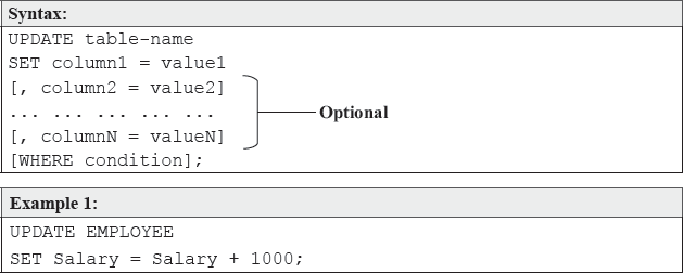
Example 1:
UPDATE EMPLOYEE
SET Salary = Salary + 1000;
The above command will update (in our case, increments) the Salary field with 1,000 for all the records.
Example 2:
UPDATE EMPLOYEE
SET Salary = Salary + 1000;
WHERE Dept = ‘RD01’;
The UPDATE command in Example 2 checks the WHERE clause first (WHERE Dept = ‘RD01’). For all records in the given table in which the WHERE clause evaluates to true, the corresponding value is updated. In the example, the WHERE condition states that the UPDATE command will increase the value of Salary field by 1,000 for only those records where department (Dept) is “RD01.” Notice in the SET, 1000 does not have quotes, because it is a numeric data type. On the other hand, “RD01” is a character data type, which requires the quotes.
The equal to (=) sign, used with the WHERE condition, is known as the comparison operator. Table 21.3 lists all the comparison operators used in SQL.
Table 21.3 Comparison Operators
| Operator | Description |
|---|---|
| = | Equal to |
| > | Greater than |
| < | Less than |
| >= | Greater than or equal to |
| <= | Less than or equal to |
| <> | Not equal to |
Example 3:
UPDATE EMPLOYEE
SET Salary = Salary + 1000, Dept = ‘RD01’
WHERE Empname LIKE ‘P%’;
The above statement is an example of multi-column update. The LIKE pattern matching operator is used in the conditional selection of the WHERE clause. It is a very powerful operator that allows the user to select only rows that are like the specified condition. The percent sign “%” is used as a wildcard to match any possible character that might appear before or after the characters specified. Hence, any Empname that begins with “P” (for example, Paul, Prince, Priya) will be considered for the WHERE condition and the salary of all these EMPLOYEEs will be incremented with 1,000 and their Dept will be updated to “RD01.”
21.4.3 DELETE Command
The DELETE statement is used to delete all or selected records from the specified table.
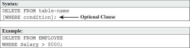
Example:
DELETE FROM EMPLOYEE
WHERE Salary > 8000;
The above statement deletes all the records from the EMPLOYEE table, which satisfy the WHERE condition. That is, records for all the EMPLOYEEs whose Salary is more than 8,000 will be deleted. Note that, if the WHERE condition is not used then all the records from the specified table will be deleted.
21.4.4 SELECT Command
Until now, we have discussed how to create, alter, and delete table. We also discussed how to insert, alter, and delete record(s) from a given table. Now comes the most important SQL command, SELECT. In fact, this command truly justifies the name of SQL. This command actually queries the database and retrieves the requested result set. SELECT allows users to retrieve data from one or more tables with various conditions. The SELECT statement allows the user to specify the desired data to be retrieved, the order to arrange the data, calculations to be performed on the data set, and many such operations. The SELECT statement has a well-structured set of clauses. We will discuss some of the most commonly used variations of SELECT in the next few sub-sections.
Before moving ahead with SELECT, let us first create a sample table with few records to execute our queries against it. Assume that the table name is EMPLOYEE and it has the following structure (Figure 21.2).
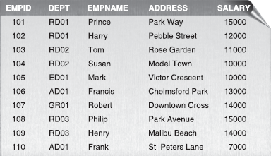
Figure 21.2 EMPLOYEE Table
SELECT Empid, Dept, Empname, Address, Salary
FROM EMPLOYEE;
The above example will display all the records of EMPLOYEE table as shown in Figure 21.2. Note that it is not mandatory to type the entire field list. You can use an asterisk (*) to substitute the field list.
SELECT * FROM EMPLOYEE;
The above SELECT command will also produce exactly the similar result, as it would do for Example 1. Remember, * is used only if one wants to display the data from all the fields. In case only selected fields are to be considered, the user has to give the name of the desired fields. For example, if one wants to display data from only two fields (say Empname and Salary), the following SELECT command must be used.
SELECT Empname, Salary FROM EMPLOYEE;
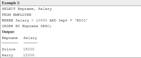
The above example illustrates conditional retrieval of data. Let us analyse the SQL statement. Notice that the WHERE condition contains an additional keyword, AND. Just like its name, AND is used to specify more than one condition along with WHERE. It tests for multiple conditions, that is, all the conditions must be true for the execution of the query. In our example, the WHERE condition specifies that only those records should be fetched whose Salary field contains a value greater than 10,000, and such records should also have “RD01” as Dept field's value. One can also use the OR logical operator to join two or more conditions, and if any of the conditions is true, the result will be displayed. For example, if OR is used in the above example, then all those records will be retrieved whose Salary field contains a value greater than 10,000, or whose Dept field's value is “RD01.”
The last clause in the above SELECT command is ORDER BY. It specifies that the fetched record set should be arranged (sorted) according to Empname field's value. In all the queries we have discussed so far, the rows of the results table have not been ordered in any way. SQL just retrieves the rows in the order in which it found them in the table. The ORDER BY clause facilitates imposing an order on the query results. By default, ORDER BY arranges the result set in ascending order (whether one uses ASC or not). Nevertheless, one can fetch records in descending order as well by adding DESC clause along with ORDER BY, as we have done in the aforementioned example. Moreover, ORDER BY can be used with more than one column name to specify the ordering of the query result.
Using Aggregate Functions: By their very nature, the databases contain large volume of data. Previously, we explored various methods of extracting specific data using the SQL. Using such queries, one can find answers for certain questions like “What are the names of all EMPLOYEEs who have a salary greater than 12,000?” Frequently, users are also interested in summarizing the data to determine trends or produce certain reports. For example, the CEO of the company may not be interested in a listing of all employee salaries, but may simply want to know the sum of the salary paid. Fortunately, ANSI/ISO SQL provides five aggregate functions to assist with the summarization of large volumes of data. In this section, we will look at functions that can be used to add and average data, count records meeting specific criteria, and find the largest and smallest values in a table.
Aggregate functions are functions that take a collection of values as input and return a single value as the output. These functions summarize the result of a query instead of reporting each detail record. SQL has five built-in aggregate functions, which are listed in Table 21.4.
Table 21.4 Aggregate Functions
| Function | Description |
|---|---|
| COUNT(column name) | Returns the number of rows of a column |
| COUNT(*) | Returns the number of selected rows |
| AVG(column name) | Returns the average or mean value of a column |
| MAX(column name) | Returns the highest value of a column |
| MIN(column name) | Returns the lowest value of a column |
| SUM(column name) | Returns the total summation of a column |
Note: Aggregate functions are also referred to as group functions.
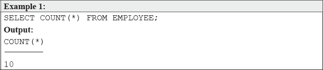
The output of the above query is 10 because there are ten records in the EMPLOYEE table. The COUNT(*) total includes all the rows addressed by the query. In case the user is only interested in obtaining the number of employees who draw a salary of more than 12,000, the WHERE clause has to be used to retrieve the specific records. For example,
SELECT COUNT(*)
FROM EMPLOYEE
WHERE Salary > 12000;
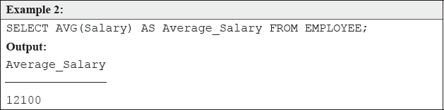
The AVG () function calculates the average or arithmetic mean of values in a column. Note that AVG() is only applied to numeric type of columns and it outputs a numeric value. SQL calculates the average by adding up all the values in the column, then dividing the total by the number of values.
Notice in the above example, we have used AS clause with AVG () function. This clause is used to specify the heading for a column in the query output. The main reason behind specifying a new heading is that all too often, the column names or the calculated expression's heading contains cryptic names that do not make sense to users outside of a company's IT department. Hence, the AS clause provides the mechanism, which allows the user to change the headings displayed in query output for enhanced readability. Notice in Example 1, the heading of the query result is “COUNT(*).” This heading may not bother the query executor, but if this result is shown to anybody else (who many not have the same SQL awareness), there may be a problem of readability. However, if the heading reads something similar to that of Example 2 (“Average_ Salary”), then anyone could easily comprehend that the figure shown is the average salary.
Note: The name used with the AS clause can be an expression but cannot contain characters (for example, spaces) that are not permitted in table field names.
Grouping Data Using GROUP BY: The aggregate functions described previously have been used to obtain grand totals. Values output by them are just like the totals that appear at the end of each column listing in a report. These functions can also be used to output subtotal values by using the GROUP BY clause in the SELECT statement. This clause lets the user to split up the values in a column into subsets. That is, the GROUP BY clause divides a table into groups of rows. This clause specifies how the retrieved records are grouped for aggregate functions, and without the GROUP BY function it would have been impossible to find the sum for each individual group of column values. Suppose the user wants to count the total number of employees department wise, then the GROUP BY clause should be used. One can group by column name when selecting character-based data, or by the results of computed columns when using numeric data types. A GROUP BY clause is most useful in statements that include aggregate functions, in which case the aggregate function produces a value for each group. To simplify, let us discuss this clause with the help of an example.
Example:
SELECT Dept, COUNT(Dept) AS No_of_Employees FROM EMPLOYEE
GROUP BY Dept;

Output:

Dept No_of_Employees
AD01 2
ED01 1
GR01 1
RD01 2
RD02 2
RD03 2
The above query first groups the rows in the EMPLOYEE table by the values in Dept. The COUNT() function then operates on each group, that is, the COUNT() function is performed for each department. The aggregate function COUNT(Dept) does not only apply to a single set of rows, but also to a group of sets of rows. The GROUP BY clause will form the group by the Dept and the COUNT(Dept) will count the number of employees with the same Dept. The GROUP BY clause is quite useful when an aggregate function is required to apply not only to a single set of rows, but to a group of sets of rows.
Note: All fields in the SELECT field list must either be included in the GROUP BY clause or be included as arguments to an SQL aggregate function.
Filtering Groups of Data Using HAVING: Previously, we have used the WHERE clause to impose conditions to filter rows. However, sometimes we may want to state a condition that applies to groups rather than rows. For example, the user may be interested only in those departments in which the average salary of employees is greater than 13,000. This can be done by using the HAVING clause with the GROUP BY to select groups according to some condition. Adding a HAVING clause to a SELECT statement sets conditions for the GROUP BY clause in a similar way the WHERE statement sets conditions for the SELECT clause. The HAVING search conditions are almost identical to WHERE search conditions. The only difference is that WHERE search conditions cannot include aggregate functions and HAVING search conditions often include these functions. Note that, HAVING can only be used with GROUP BY Without the HAVING, it would not be possible to test for function result conditions. It can include as many filter conditions as needed, connected with the AND or OR operator.
Example:
SELECT Dept AS Department, AVG(Salary) AS Average_Salary
FROM EMPLOYEE
GROUP BY Dept
HAVING AVG(Salary) > 13000
ORDER BY AVG(Salary);

Output:
Department Average_Salary
__________ _______________
RD01       13500
GR01       14000
RD03       14500
In the above SQL query, firstly, the rows will be grouped according to Dept and the average Salary of each group will be calculated. Then the HAVING clause will set the filter condition that groups must meet to be included in the query results, that is, the average Salary of each Dept should be greater than 13,000. Finally, the results will be displayed according to the ascending order of the average Salary.
Using Character Functions: There are certain situations in which the user might wish to format the data in a particular manner. For character-type data, there are several character and string functions available, such as concatenation, trim, and substring functions. Note that different DBMS vendors have different string function implementations. Table 21.5 covers the most common character functions.
Table 21.5 Character Functions
| Function | Description |
|---|---|
| LEN(expression) or LENGTH(expression) | Returns number of characters in the specified expression |
| INITCAP(expression) | Converts alphabetical character values to upper case for the first letter of each word, all other letters in lower case |
| LOWER(expression) or LCASE(expression) | Converts alphabetical character values to lower case, that is, the characters A–Z will be translated to the characters a–z |
| UPPER(expression) or UCASE(expression) | Converts alphabetical character values to upper case, that is, the characters a–z will be translated to the characters A–Z |
| LTRIM(expression) | Removes spaces from the beginning of expression |
| RTRIM(expression) | Removes spaces from the end of expression |
| CONCAT(first_string, second_string) | Joins two character expressions into a single string value |
| REPLACE(searched_string, search_key, replacement_string) | Replaces all occurrences of search_key in searched_string with replacement_string. Note the replacement_string is optional and if it is left out, each occurrence of the search_key on the string to be searched is removed and is not replaced with anything |
| SUBSTR(target_string, start_pos, end_pos) or SUBSTRING (target_string, start_pos, end_pos) | Extracts a specified portion of the character expression (target_string) on which it is operating. start_pos is the position of the first character to be output and end_pos is the number of characters to show |
SELECT Empname, LEN(RTRIM(Empname)) AS Name_Length
FROM EMPLOYEE
WHERE Dept = ‘RD03’;
Output:
Empname Name_Length
_______ ___________
Philip   6
Henry    5
In the above example, LEN() function is used to ascertain the length of Empname column's values. We have used the RTRIM() function along with LEN() because while creating the EMPLOYEE table, the Empname column was stated as fixed-length character data type, that is, CHAR(15) (refer Section 21.3.1). Consequently, this column will automatically add spaces if the inserted value's length is not equal to 15. To be precise, if the value is “Prince,” actually it is stored in the table as “Prince-------” (- denotes space). In such a case, if only LEN() command is used, it will display 15 as output for all the rows irrespective of the actual length of Empname's value. However, had we created the column with the VARCHAR, we would not have to use the RTRIM() function. In that case, simply using the LEN() would have accomplished the same output.
Example 2:
SELECT UCASE(Empname)
FROM EMPLOYEE
WHERE Salary > 13000;

Output:

UCASE(Empname)
PRINCE
ROBERT
PHILIP
HENRY
In the above example, UCASE() function is used to display the values of Empname column in upper case. Note that since UCASE() is used with SELECT, it actually does not convert the column's value in the table. For that, you will have to use the UPDATE command.
SELECT Empname FROM EMPLOYEE
WHERE SUBSTR(Empname,1,4) = ‘Fran’;

Output:

Empname
_______
Francis
Frank
In the above example, the WHERE condition selects only those rows from the EMPLOYEE table for which the employee name (Empname) starts with the word “Fran.” Here 1 specifies the position in the string from where to start the substring and 4 specifies the length of the substring.
Using Mathematical Functions: Just as the character functions, SQL has some inbuilt mathematical functions that are used to retrieve data which involve mathematics. Most DBMSs provide arithmetic functions similar to the functions covered in Table 21.6.
Table 21.6 Mathematical Functions
| Function | Description |
|---|---|
| ABS(expression) | Returns the absolute value of the expression |
| CEILING(expression) or CEIL(expression) | Returns the smallest integer value greater than or equal to expression |
| FLOOR(expression) | Returns the largest integer value less than or equal to expression |
| ROUND(expression, length) | Returns the expression rounded to length places right of the decimal point. If length is negative, expression is rounded to the absolute value of length places to the left of the decimal point |
| SQRT(expression) or SQR(expression) | Returns the square root of the expression |
| POWER(expression, p) | Raises the expression to the power of p |
| EXP(expression) | Returns the exponential function of expression |
| LOG(expression) | Returns the natural logarithm of expression |
| LOG10(expression) | Returns the base-10 logarithm of expression |
| SIN(expression), COS(expression), TAN(expression) | Returns the sine, cosine, and tangents of the specified expression, respectively |
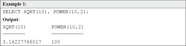
In the above example, the SQRT() function evaluates the square root value of 10 and the POWER() functions raise the value of 10 to the power of 2.
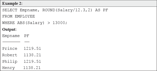
The above example illustrates the use of mathematical functions on a table's column. The ROUND() function rounds off the specified numerical expression (Salary/12.3) to 2.
21.5 QUERYING MULTIPLE TABLES (SQL JOINS)
All the queries until this point were based on a single table only. However, SQL possesses a very powerful feature of gathering and manipulating data from across several tables. Without this feature, the database creator would have to store all the data elements necessary for each application in one table. Moreover, without common tables, the same data may have to be stored in several tables To solve this problem, SQL introduced the concept of joins, which enables the database designer to design smaller, more specific tables that are easier to maintain than a single larger table.
THINGS TO REMEMBER
SQL Joins
A join combines records from two or more tables in a relational database. In other words, join makes relational database systems “relational.” There are three types of joins, namely, inner join, left outer join, and right outer join. These joins determine records that appear when a query is executed to show information from two tables. All these joins work by linking records on a key field.
Remember, we discussed the concept of foreign keys in the last chapter. A foreign key is a column in a table where that column is a primary key of another table, which means that any data in a foreign key column must have corresponding data in the other table where that column is the primary key. In DBMS terms, this correspondence is known as referential integrity. The join condition actually puts the concept of foreign key in practical use to link data from two or more tables together into a single query result—from one single SELECT statement. Good database design suggests that each table lists data only about a single entity, and detailed information can be obtained in a relational database, by using the join operation with other tables. A “join” can be recognized in a SELECT statement if it has more than one table after the FROM keyword.
Syntax:
SELECT list-of-columns
FROM table-name1 [AS alias-name], table-name2 [AS alias-name]
[WHERE table1_keyfield = table2_foreign_keyfield];
Before going ahead with joins, let us create two tables so that we can “join” them to retrieve data (Figure 21.3).
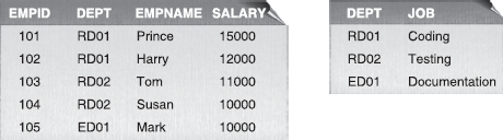
Figure 21.3 EMPLOYEE and DEPARTMENT Tables
Now, you might think that a natural extension of the SELECT statement is the following:
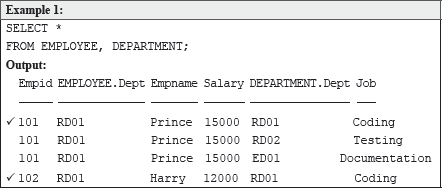
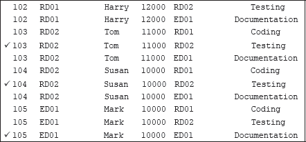
Although the above query is perfectly correct, but obviously, it did not retrieve the desired result. Every single row of the first table has been joined with each row of the second table, not just the rows that we think should correspond (the marked records). This is called a Cartesian join or cross-join and can rapidly generate enormous tables. According to this join, if there are two tables, each with a thousand rows, then 1,000 × 1,000 = 1,000,000 rows are displayed. Hence, to reduce the number of rows, and to get the desired result, simply use a WHERE clause to join the tables on the matching column, thus:
In the above query, there are mainly two issues. Firstly, the matching columns (Dept) are used along with their table names with a dot operator (.). This is done to clearly mention the table to which the columns belong. In any case, if the table names are not mentioned along with the column, SQL will generate an error. Secondly, an asterisk (*) is used to display all the columns from both joined tables to be listed. However, just like normal SELECT statements, we can use specific column names as well.
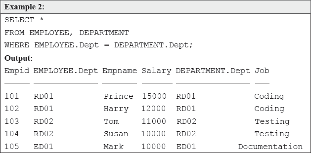
Example 3:
SELECT Empid, EMPLOYEE.Dept, Empname, Job
FROM EMPLOYEE, DEPARTMENT
WHERE EMPLOYEE.Dept = DEPARTMENT.Dept;
Observe that in the above query, the table names are not used with those columns that are not common in joined tables. Although the uncommon column names can also be listed along with their table names, it is up to the user discretion. Nevertheless, the common column(s) must be listed along with their table names. Thus, the above query can also be written as:
SELECT EMPLOYEE.Empid, EMPLOYEE.Dept, EMPLOYEE.Empname, DEPARTMENT.Job
FROM EMPLOYEE, DEPARTMENT
WHERE EMPLOYEE.Dept = DEPARTMENT.Dept;
Just as we have changed the column heading using the AS clause, a table can also have an alias name in the FROM clause. The alias is used wherever the table or column name would be used in other parts of the query. When an alias is defined, we can use the alias (instead of relation name) to refer to whose attribute we want to use in the query. For example, the previous join query can be rewritten as:
SELECT E.Empid, E.Dept, E.Empname, D.Job
FROM EMPLOYEE E, DEPARTMENT D
WHERE E.Dept = D.Dept;
21.5.1 Combining Queries Using UNION
There are occasions where the user might want to see the results of multiple queries together, combining their output. In such situations, UNION can be used. UNION is somewhat similar to “join” as they are both used to relate information from multiple tables. UNION adds the result of a second SELECT clause to the table created by the main SELECT command. One restriction of UNION is that all corresponding columns need to be of the same data type (numeric columns must correspond to numeric columns, string columns with string columns). Moreover, when using UNION, only distinct values are selected. For example, to get the list of department IDs, the following query is used.
Example:
SELECT Dept FROM EMPLOYEE
UNION
SELECT Dept FROM DEPARTMENT;

Output:

Dept
____
RD01
RD02
ED01
Note: With UNION, only distinct values are selected. To select all the values, use UNION ALL.
21.6 NESTING SELECT STATEMENTS (SUBQUERY)
A subquery is SELECT statement that nests inside the WHERE clause of another SELECT statement. In relational databases, there may be many situations when the user has to perform a query, temporarily store the result(s), and then use this result as part of another query. This nesting of queries is known as subquery. The basic idea behind it is that instead of a “static” condition, the user can insert a query as part of a WHERE clause. The main reason of using subquery is that it breaks down a complex query into a series of logical steps, and as a result, solves a problem with a single statement.
Syntax:
SELECT list-of-columns FROM table-name
WHERE attribute conditional operator
(SELECT list-of-columns FROM table-name
[WHERE condition]);
While creating a subquery, the following guidelines should be considered.
- The subquery must be on the right side of the conditional operator.
- The subquery must be enclosed within parenthesis.
- Multiple select subqueries can be combined (using AND, OR) in the same statement, but it is not advisable.
- When a subquery is part of a WHERE condition, the SELECT clause in the subquery must have columns that match in number and type to those in the WHERE clause of the outer query.
Example:
SELECT Empname, Salary FROM EMPLOYEE
WHERE Salary = (SELECT MIN(Salary) FROM EMPLOYEE);

Output:
Empname Salary
_______ ______
Susan 10000
Mark 10000
In the above example, the subquery (SELECT MIN(Salary) FROM EMPLOYEE) will return 10,000 as the result. This result will then be used by the main query to display the queried output.
Let Us Summarize
- SQL is an ANSI/ISO standardized computer language for Defining and manipulating data sets from a database. Using SQL, the user can retrieve data from a database, create databases and database objects, add data, modify existing data, and perform other, more complex functions.
- SQL is a medium of communicating to the DBMS what the user wants it to do. SQL statements describe what data to be retrieved, rather than specifying how to find the data. The DBMS takes care of locating the requested data from the database.
- Typically, there are two parties (front-end and back-end), which together use the SQL to process the requested query. The front-end sends an SQL statement (containing instructions to create, read, change, or delete data) across a connection to a back-end, which holds the data.
- SQL can be used in two different ways: either SQL commands can be typed at the command line directly or it can be embedded in a host language like COBOL or C. The first method is known as interactive SQL and the second method is called embedded SQL.
- The main characteristics of SQL are that it is an ANSI/ISO standard computer language and not owned or controlled by any single company. It is a cross-platform language, that is, the same SQL statements can be used on a multitude of hardware/software platforms. SQL is easy to learn and understand and requires less programming since most of the queries are of single line. However, SQL is not a complete programming environment because there is no front-end built into it; neither does it have a back-end.
- The SQL standard specifies data definition, data manipulation, and other associated facilities of a DBMS that supports the relational data model. ANSI standardized SQL in 1986, and ISO standardized it in 1987. After that, SQL was revised as SQL89 (or SQL1), SQL92 (or SQL2), SQL99 (or SQL3), SQL2003, SQL2006, and SQL2008.
- SQL input consists of a sequence of commands, and each command is composed of a sequence of tokens (keyword, identifer, or literal), terminated by a semicolon. Note that, SQL is not case sensitive.
- The CREATE TABLE command is to define the table's structure.
CREATE TABLE table-name( <column1> <data-type>, <column2> <data-type>, ... ... ... ... <columnN> <data-type>); - The ALTER TABLE command is used to change the structure of an existing table.
ALTER TABLE table-name <ADD | MODIFY | DROP column(s)>; - The DROP TABLE command removes the table definition (with all records).
DROP TABLE table-name; - The INSERT command is used to add records in a table.
INSERT INTO table-name ( column1, column2, ..., columnN) VALUES (value1, value2, ..., valueN); - The UPDATE command is used to make changes to the data in the database.
UPDATE table-name SET column1 = value1 [column2 = value2, ... ... ... ... columnN = valueN] [WHERE condition]; - The DELETE command is used to delete all or selected records from the specified table.
DELETE FROM table-name [WHERE condition]; - The SELECT command is used to query the database to retrieve the requested result set. It allows users to retrieve data from one or more tables with various conditions. It also allows the user to arrange the data, to perform calculations on the data set, and many such operations.
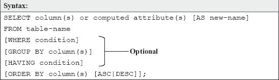
SELECT column(s) or computed attribute(s) [AS new-name] FROM table-name [WHERE condition] [GROUP BY column(s)] [HAVING condition] [ORDER BY column(s) [ASC | DESC]]; - ANSI/ISO SQL provides five aggregate functions to assist with the summarization of large volumes of data.
- COUNT() returns number of rows of a column.
- AVG() returns the average or mean value of a column.
- MAX() returns the highest value of a column.
- MIN() returns the lowest value of a column.
- SUM() returns the total summation of a column.
- SQL provides several character and string functions, such as:
- LEN()/LENGTH() returns the length of the specified string.
- LCASE()/LOWER() converts alphabetical character values to lower case.
- UCASE()/UPPER() converts alphabetical character values to upper case.
- INITCAP() converts alphabetical character values to upper case for the first letter of each word, all other letters in lower case.
- LTRIM() removes spaces from the beginning of expression.
- RTRIM() removes spaces from the end of expression.
- CONCAT() joins two character expressions into a single string value.
- REPLACE() replaces all occurrences of a search key from the searched string with a replacement key.
- SUBSTR()/SUBSTRING() extracts a specified portion of the character expression on which it is operating.
- SQL provides several mathematical functions, such as:
- ABS() returns the absolute value of the expression.
- CEILING()/CEIL() returns the smallest integer value greater than or equal to expression.
- FLOOR() returns the largest integer value less than or equal to expression.
- ROUND() returns the expression rounded to length places right of the decimal point.
- SQRT()/SQR() returns the square root of the expression.
- POWER() raises the expression to the specified power.
- EXP() returns the exponential function of expression.
- LOG() returns the natural logarithm of expression.
- LOG10() returns the base-10 logarithm of expression.
- SIN(), COS(), TAN() returns the sine, cosine, and tangents of the specified expression, respectively.
- SQL possess a powerful feature of gathering and manipulating data from across several tables by using joins. A join can be recognized in a SELECT statement if it has more than one table after the FROM keyword.
SELECT list-of-columns FROM table-name1 [AS alias-name], table-name2 [AS alias-name] [WHERE table1_keyfield = table2_foreign_keyfield]; - UNION adds the result of a second SELECT clause to the table created by the main SELECT command.
- A subquery is SELECT statement that nest inside the WHERE clause of another SELECT statement.
SELECT list-of-columns FROM table-name
WHERE condition
SELECT list-of-columns FROM table-name
[WHERE condition]
Exercises
Fill in the Blanks
- SQL-based queries collect rows having same value in the...............clause in one cluster.
- The language used for data modifcation is known as...............
- ...............clause is used to eliminate some groups from a SELECT query.
- The technique of passing the result of inner query to outer query is known as...............
- When SQL statements are incorporated into programs written in general-purpose programming language, it is known as...............
- The part of a software program that a user sees and interacts with is known as...............
- SELECT statements describe...............to retrieve, rather than...............to retrieve.
- The three main SQL standards are..............., ..............., and ...............
- Group functions are also known as ............... functions.
- Instead of specifying entire column list, ...............can also be used to select all columns.
Multiple-choice Questions
- You want to run a SELECT command that lists all employees by the ascending order of their names. What clause would you include in the query to do the ordering?
- LIST ASC BY EMPLOYEE.Name
- ORDER BY EMPLOYEE.Name
- SORT BY EMPLOYEE.Name
- WHERE EMPLOYEE.Name ASC
- A language that is used to specify the database scheme through a set of definitions is called...............
- SQL
- DML
- DDL
- ISO
- Which of the following is an aggregate function?
- PLUS
- ABS
- MINIMUM
- COUNT
- SQL is...............type of language.
- Low level
- Procedural
- High level
- Non-procedural
- The query: SELECT * FROM STUDENT WHERE Course LIKE ‘%A’; will...............
- Display all the courses that begin with the letter “A”
- Display all the courses that end with the letter “A”
- Display only those courses that contain numeric digits in the beginning
- Produce an error because the query is incorrect
- What does SQL stand for?
- Structured question language
- Structured query language
- Structured question language
- Structured quarantine language
- Which SQL command inserts new data in a database?
- INSERT
- NEW
- ENTER
- ADD
- ...............command extracts data from a database.
- OPEN
- EXTRACT
- GET
- SELECT
- To select all the records from a table named “STUDENT,” where the First_Name is “Mark” and the Last_Name is “Edward,” which of the following SQL statement should be used?
- SELECT First_Name=“Mark” Last_Name=“Edward” FROM STUDENT
- SELECT * FROM STUDENT WHERE First_Name=“Mark” AND Last_Name= “Edward”
- SELECT “Mark” “Edward” FROM STUDENTFirstName, STUDENTLastName
- It is not possible using SQL query.
- ...............function returns the smallest integer value greater than or equal to the expression.
- FLOOR(expression)
- CEILING(expression)
- ABS(expression)
- EXP(expression)
State True or False
- In SQL, columns of different tables can have the same name.
- ODBC is an example of back-end.
- SQL join creates a new table by joining two or more tables.
- SELECT Name Item Amount FROM CUSTOMER; is an invalid query.
- SQL is owned jointly by IBM and Oracle.
- The maximum limit of a VARCHAR data type is 256 characters.
- In SQL SELECT, if there are more than one table after the FROM keyword, it represents a join.
- SQL is case-insensitive language.
- The AND operator displays a record if any conditions listed are true. The OR operator displays a record if ALL of the conditions listed are true.
- The SQL REMOVE command deletes data from a database.
Descriptive Questions
- How SQL is used in a DBMS to retrieve the data?
- Discuss the characteristics of SQL in brief.
- Consider the following tables:
Structure of EMPLOYEE Table
Field Name Data Type Description EmpID Numeric Employee's ID number DeptID Numeric Department's ID number Emp_Name Character Employee's name Employee's Salary Numeric Salary Dept_ID Data Type Description DeptID Numeric Department's ID number Dept_Name Character Department's name Supervisor Character Department supervisor's name Give the SQL expressions for the following queries with respect to the above tables.
- Find names for all employees who work for the “Accounts” department.
- For each employee, retrieve the employee's name and the name of his/her supervisor.
- How many employees work in the “Accounts” department?
- What are the maximum, minimum, and average salary in the “Accounts” department?
- Retrieve the department names for each department in which more than two employees work.
- Modify the database so that “Michael” is assigned to the “Accounts” department.
- Give all employees of “Sales” department a 10% rise in salary.
- Delete all rows for employees of “Apprentice” department.
- There is a table named “PEOPLE” that has four columns: Country, Continent, Area, and Population. The first two columns are character types and the last two columns are numeric types. Now write the appropriate SQL queries for the following:
- List the countries that have at least 5,00,000 people. [Show Country, Population]
- Identify the countries, which have the word “United” included in their names.
- List each country name where the population is larger than “United States.”
- For each continent, show the number of countries with populations of at least 10 million.
- List the continents with total populations of at least 100 million.
ANSWERS
Fill in the Blanks
- GROUP BY
- DML
- HAVING
- Subquery
- Embedded SQL
- Front-end
- What, How
- SQL89, SQL92, SQL99
- Aggregate
- Asterisk (*)
Multiple-choice Questions
- (b)
- (c)
- (d)
- (d)
- (b)
- (b)
- (a)
- (d)
- (b)
- (b)
State True or False
- True
- False
- False
- True
- False
- False
- True
- True
- False
- False