
Chapter 5
Prostate Cancer: PSA, AR, and ADT Dynamics
5.1 Introduction
The prostate is a walnut-shaped and sized organ that envelops the urethra. Accounting for at most 0.1% (and as little as 0.01%, depending upon the individual) of the male body mass, it remains something of a mystery why neoplasms of this tiny organ contribute so greatly to cancer burden. Prostate cancer (PC) accounts for 25% of new cancer diagnoses and 10% of cancer deaths in American men [28].
Prostate cancer incidence and mortality vary widely worldwide, with those in the West far more likely to die of the disease. The natural history of prostate cancer spans decades, and can begin in the third or fourth decade of life, as shown by autopsies of men who died of other causes. Most men develop prostate enlargement at some point in life, and by age 90, 90% of men worldwide have developed some form of preclinical prostate cancer [59]. While it is diagnosed more often than any other cancer (in men), cancer aggressiveness varies widely between individual patients, and a majority of those diagnosed will not actually die of the disease. Over 90% of prostate cancer cases are diagnosed at local or regional stages for which survival approaches 100% [28].
The long preclinical phase of this neoplasm suggests a typically slow evolutionary progression toward the malignant phenotype; how ecological factors drive this selective process is not known. Indeed, the role of androgens in the prostate cancer etiology is controversial; we discuss this in some depth in Section 5.4.
Since the late 1980s, prostate cancer screening is typically done by measuring the serum prostate specific antigen (PSA). PSA is a proteinase produced by healthy prostate epithelium, and it is not an intrinsic marker of cancer. Normally, only a very small amount of PSA leaks through the prostate interstitium into the blood. Thus, elevated levels of blood PSA often correlate with prostatic hyperplasia.
While PSA levels have been generally understood to correlate with prostate neo-plasia mass, the efficacy of PSA screening is unclear and remains very controversial. A recent study by the U.S. Preventive Services Task Force [33] concluded that the natural history of PSA-detected cancer is poorly understood, and screening can cause significant psychological harm. The task force recommended that men over 75 not be screened, as potential harm outweighed the benefits, while the evidence for those under 75 was insufficient to recommend for or against testing. In light of this controversy, we open this chapter with several simple clinical [9, 66] and dynamical models [61, 67] relating serum PSA and tumor growth dynamics.
Here, as elsewhere throughout this text, we invoke Theodosius Dobzhansky’s rule that “nothing in biology makes sense except in the light of evolution” [13] (see also Chapter 1) to help explain the biology and clinical behavior of prostate cancer. This neoplasm’s physiology is intimately linked to androgens (e.g., testosterone), the male sex hormones. Androgens are essential resources for survival and development of healthy prostate tissue. These hormones mediate proliferation, apoptosis, oxidative stress, and perhaps inflammation in the prostate. Thus they play a central role in modulating selection for cancerous cells.
In this chapter we investigate a multi-scale model of prostate cancer that includes dynamics of the concentrations of serum testosterone, intracellular testosterone and dihydrotestosterone (DHT), the androgen receptor (RA) and its complexes with the two androgens. The primary observable variable in both model and clinic is serum PSA. We will then apply this model to study androgen ablation therapy, which is a treatment of last resort for advanced tumors. Since healthy prostate epithelial cells rely on androgen, it is not surprising that prostatic epithelial tumors—the main type of prostate cancer—rely on androgens for growth and survival, or that androgen blockade (via castration) essentially invariably causes tumor regression. This type of hormone therapy is called androgen deprivation therapy (ADT) or androgen suppression therapy. The androgen suppression can be applied continuously or intermittently. Unfortunately, in either case, resistance to the treatment inevitably evolves as androgen insensitive tumor clones arise and become the dominant phenotypes. The mechanism appears to be natural selection, as clones that have less need for androgen become favored in the competition for this hormonal “resource.”
Unfortunately, due to the lack of clinical data and the complexity of our comprehensive multi-scale model, we are unable to perform any serious model validation. Nevertheless, some very limited clinical data sets can be employed to estimate a subset of the parameters in our model. In the next chapter, we explicitly and mechanistically address nutrient-limited cell growth and competition in the context of prostate cancer dynamics subject to intermittent ADT. By focusing on just the cell and population scales, we are able to formulate more tractable models and validate them with clinical data. Understanding the evolution of aggressive prostate cancer in response to androgen ablation therapy has also been the focus of several mathematical models. If a model can accurately describe this evolution, then it could serve as a guide for rational treatment strategies that minimize evolution to an androgen-independent phenotype.
5.2 Models of PSA kinetics
The value of PSA in screening for prostate cancer is controversial, but in cases of confirmed cancer, serum PSA correlates with tumor volume across patients. However, in individual cases, serum PSA correlates poorly with tumor volume and prognosis. For example, grouping cancers into volume groups can yield excellent correlation between volume group and serum PSA, but the variance is so large that serum PSA cannot be used to predict individual tumor volumes [39].
Several other metrics have diagnostic and prognostic value, and other PSA kinetic parameters have been studied, including PSA velocity (the rate of PSA change), PSA density (the ratio of PSA to prostate volume), and the PSA doubling time (or equivalently, the relative PSA velocity). There has been a great deal of interest in predicting outcomes in response to therapy on the basis of pre-treatment findings. To this end, a number of statistical models have been employed that use metrics such as serum PSA, PSA density, PSA velocity, positive digital rectal examination (DRE), prostate volume in transrectal ultrasound, Gleason grade of biopsy samples, and patient age. Such predictive aids are referred to as nomograms, and a great number have been published [53].
Response to therapy, survival and quality of life are what is ultimately of clinical interest, and nomograms designed to predict tumor volume or pathological grade are only of secondary clinical interest, as such metrics must then themselves be related to survival and therapeutic response. However, we restrict our consideration to how PSA kinetics predict tumor volume and changes in tumor volume.
5.2.1 Vollmer et al. model
As an example, we begin with the study by Vollmer et al. [66], who present a model that tracks serum PSA in untreated prostate cancer (i.e., watchful waiting). These researchers describe serial measurements of PSA with a log-linear model:
log(y(t))=a+bt, (5.1)
where y(t) represents serum PSA. This is easily transformed to the familiar case of exponential growth,
y(t)=y0ebt, (5.2)
where y0 = ea. Parameter a is referred to as PSA amplitude, and
b=ln(2)/(PSA doubling time)
is referred to as the relative PSA velocity. If one wishes to relate it to clinically measured PSA velocity and serum PSA, it can also be expressed as
b=dy/dty. (5.3)
Vollmer et al. concluded that PSA amplitude together with the relative PSA velocity best predicted outcomes. The key result of this work is that, at least in slower growing, untreated cancers, the underlying dynamic describing the change in serum PSA is exponential growth. Moreover, other authors have found that PSA relative velocity (or doubling time) is a strong marker of disease progression [38], consistent with the notion that serum PSA changes parallel changes in tumor growth, which is typically characterized by a doubling time.
5.2.2 Prostate cancer volume
Serum PSA is a marker for PSA production by both healthy and cancerous prostate cells. A number of simple mathematical and empirical relationships can be derived relating PSA to prostate cancer volume. For example, D’Amico et al. [9] derived the “calculated prostate cancer volume” using simple mathematics to relate prostate volume, as measured by ultrasound (which includes tumor and healthy cells), cancer Gleason grade in biopsy cores, and serum PSA to estimate volume of the actual tumor. Let serum PSA concentration be y, the volume of benign prostate epithelium be Vb, the volume of cancerous prostate tissue be Vc, and represent the per-unit volume contribution of PSA to the serum for benign and cancerous tissue by c1 and c2, respectively. The fundamental relationship between these is
y=c1Vb+c2Vc, (5.4)
which implies that
Vc=y−c1Vbc2. (5.5)
D’Amico et al. refer to the numerator as the “cancer-specific PSA,” as it is the total PSA minus the PSA contribution from benign tissues; the quantity c1Vb is called the “PSA from benign epithelial tissue.” The latter quantity is itself determined as a function of the prostate volume as determined by transrectal ultrasound and the epithelial fraction of the prostate. Letting Vp represent the total prostate volume and ϕ be the epithelial fraction gives
Vb=ϕVp. (5.6)
Finally, cancer volume is calculated in terms of serum PSA, prostate volume on ultrasound, prostate epithelial fraction, and PSA leak from benign and tumor tissue as follows:
Vc=y−c1ϕVpc2. (5.7)
Lepor et al. [32] measured a PSA increase of 0.33 ng/ml for every additional cm3 of prostate epithelial tissue, a value D’Amico et al. used to calculate c1. A more recent measurement by Fukatsu et al. [17] places this value at 1.27 ng/ml per cm3 of epithelium.
The epithelial fraction was measured by Marks et al. [36] in 20 prostate samples from men with benign prostatic hyperplasia (BPH) and ranged from 0.117 to 0.308 with an average of 0.199, implying that ϕ ≈ 0.20. Thus, from the simple relationship (5.4) it follows that prostate cancer volume can be estimated using several empirical measurements and parameters. However, these parameters themselves are functions of lower-level dynamical parameters, and variation between them may still limit the predictive ability of the “calculated prostate cancer volume” in individuals. Although in their original work, D’Amico et al. found the calculated prostate cancer volume to be a much better predictor of actual volume than was serum PSA, a subsequent study failed to validate this finding [7].
Using newer estimates of PSA per cm3 of epithelial tissue, or assuming different epithelial fractions depending upon whether BPH is present, are possible modifications that could improve the ability of the calculated prostate cancer volume to predict the actual cancer volume. But ultimately, it is not surprising that such a model cannot predict individual tumor volumes, as the parameters c1 and c2 are in reality functions of individually variable dynamical parameters, as we shall see in the following section.
5.3 Dynamical models
Serum PSA concentration is determined by the balance between input from the prostate into the serum compartment and clearance from this compartment. The parameters c1 and c2 in equation 5.4 then represent the aggregate result of this flux balance.
Two simple dynamical models have been proposed to account for the dynamics underlying serum PSA kinetics. The first, by Swanson et al. [61], considers serum PSA dynamics as a function of tumor growth. A later model by Vollmer and Humphrey [67] focuses on production of PSA in the prostate compartment, PSA transfer to the serum, and its subsequent clearance from this compartment. Below we discuss these models, their construction, and the insight they give into PSA dynamics.
5.3.1 Swanson et al. model
Because serum PSA level and prostate cancer volume correlate poorly at individual patient level, Swanson et al. [61] proposed a simple dynamical model to examine the relationship between these two quantities. In their model, serum PSA is produced by healthy and cancerous cells at different rates and is eliminated from the serum by first-order kinetics. Serum PSA is represented by y(t) (in ng/ml), and Vh and Vc(t) (both in mm3) give the volume of healthy and cancerous prostatic cells, respectively. Note that Vh is assumed to be constant. These considerations yield the following linear model:
dydt=βhVh+βcVc(t)−ky(t). (5.8)
The tumor is assumed to grow exponentially, so
Vc(t)=V0ept. (5.9)
We have βh as the rate at which PSA is produced by healthy prostate, βc the rate of PSA production for cancerous prostate, and k the rate at which PSA is cleared, while ρ is the per-unit-volume rate of tumor volume increase, which is related to the doubling time, td, by td = ln(2)/k.
This model can be criticized for its simplicity; the assumption of exponential tumor growth clearly cannot hold for all time, and any number of background biological processes are neglected. However, it is important to keep the issue that motivates the model in mind, which is the relationship between tumor volume and PSA serum dynamics. Thus, the simple model can still generate important insight in this area, and can potentially be more insightful than a more complicated model. Furthermore, this model takes into account the underlying biological process (i.e., tumor growth) determining PSA dynamics. This contrasts with the widely employed statistical nomograms, although the scope of the two approaches differ.
Due to its importance for the scientific predictions, we devote significant space to the parameter estimation process. This model was parameterized using in vivo data from a nude (athymic) mouse xenograft model of prostate cancer by Ellis et al. [15]. Because it is a xenograft (human cancer implanted into an immune-deficient mouse), Vh = 0. Parameters V0 and k (from PSA half-life) are given by Ellis et al., while Swanson et al. estimated the tumor growth rate, ρ, from time-series data for tumor volume (see Table 5.1).
Parameters (P) obtained from 3 human-derived mouse xenograft sublines (LuCaP 23.1, 23.8 and 23.12) used for Swanson’s PSA model.
P |
LuCaP 23.1 |
LuCaP 23.8 |
LuCaP 23.12 |
Units |
|---|---|---|---|---|
ρ |
0.0655 |
0.0504 |
0.0487 |
day−1 |
βh |
0 |
0 |
0 |
ng ml−1 |
mm−3 day−1 |
||||
βc |
1.7210 |
2.1841 |
6.9722 |
ng ml−1 |
mm−3 day−1 |
||||
k |
1.2896 |
1.2896 |
1.2896 |
day−1 |
V0 |
20–25 |
20–25 |
20–25 |
mm3 |
Vh |
0 |
0 |
0 |
mm3 |
To determine PSA production rate, Swanson et al. used the analytical solution for y(t) in conjunction with PSA:volume ratios reported in [15]. Here is the procedure. First, note that
y(t)=βcρ+k(Vc−V0e−kt), (5.10)
satisfies dy/dt = βcVc − ky, y(0) = 0. Suppose that asymptotically, y and Vc. approach constant values. As t → ∞, e−kt → 0, and we have that
yVc=βcρ+k. (5.11)
Since the ratio y/Vc and parameters ρ and k are known for all cell lines, it is now a simple matter to calculate estimates for βc Ellis et al. reported PSA indices (PSA:tumor volume ratios) for cell sublines of human prostate cancer derived from three different metastatic sites in a single patient (LuCaP 23.1, LuCaP 23.8 and LuCaP 23.12). These ratios were 1.27, 1.63, and 5.21 ng ml−1 mm−3 for LuCaP 23.1, 23.8, and 23.12, respectively, yielding βc = 1.7210, 2.1841, and 6.9722 ng ml−1 mm−3 day−1. Table 5.1 gives all parameter values for these mouse xenografts, while Table 5.2 gives likely values for human prostate cancer as derived below.
Likely parameter values in man under Swanson’s PSA model framework.
Swanson et al. suggested that the dimensionless ratio µ = k/ρ determines the usefulness of the PSA level in predicting tumor volume, and therefore differences in tumor growth rates can explain the disconnect between measured PSA level and tumor volume. However, on closer examination, while the data supports the notion that normal variations in parameter value between individuals can explain the poor correlation between PSA and tumor volume, the aggregate parameter µ is not the key parameter. Rather, we argue that k, the PSA clearance rate, and βc, the PSA production rate, are much more important.
Parametrization of human prostate cancer. To determine if and how parameter differences impact the PSA:volume ratio, we must first determine the biologically reasonable parameter range for human prostate cancers. Berges et al. [4] determined tumor doubling times for prostate cancers at various stages in their evolution. For non-metastatic cancer, the smallest doubling time was 154 ± 22 days (ρ = 0.0045 day−1). The smallest doubling time overall was for lymph node metastases in hormonally untreated cancer, at 33 ± 4 days (ρ = 0.021 day−1). The largest doubling time was 577 ± 68 (ρ = 0.0012 day−1) for low-grade localized cancer.
In [4], it is reported that athymic (nude) mice clear PSA seven times faster than humans. Since nude mice were used in [15], this implies a human half-life of 3.76 days. This corresponds to estimates in the literature that all range between 1.72 days and 3.95 days [19, 34], giving k = 0.1754 to 0.4030 day−1.
For the sake of completeness, we note that normal prostate volume in younger men is around 20 cm3. Vesely et al. [65] measured non-cancerous prostate volumes and serum PSA mainly in older men. Prostate volume ranged from 10 to 157 cm3, with an overall average of 40.1 ± 23.9. These values correlate with age: mean prostate size for men under 54 years was 27.5 cm3, while the mean for men under 80 was 48.2 cm3. Mean serum PSA follows a similar pattern. For all men in the study, serum PSA averaged 3.9 f 4.2 ng/ml, with means of 1.5 ng/ml for men under 54 and 5.4 ng/ml for men under 80. Assuming a stroma to epithelium ratio of 2:1 for a healthy prostate [60], this gives Vh = 3333 to 52333 mm3. Setting Vc = 0, and assuming a steady state yields the simple relationship,
βh=kyVh. (5.12)
Using Vh = 9167 mm3, y = 1.5 ng/ml (values for men under 54), and k ∈ [0.1754, 0.4030] yields βh = 2.870 × 10⁻⁵ to 6.595 × 10⁻⁵ ng ml−1 mm−3 day−1. Using Vh = 16067 mm3, y = 5.4 ng/ml (values for men under 80), and k ∈ [0.1754, 0.4030] yields βh = 5.895 × 10⁻⁵ to 1.354 × 10⁻⁴ ng ml−1 mm−3 day−1. These parameter values suggest that older men produce PSA at a higher rate per volume of prostate tissue than do younger men. Further more, benign prostatic hyperplasia, common in older men, results in a greater stroma:epithelium ratio [60]. Increasing this ratio yields an even larger βh value, suggesting that our estimate is a lower bound.
Predictions. Using the parameter estimates just derived, it is a simple matter to show that while varying the tumor growth rate does have a small effect on the PSA:tumor volume ratio, this effect is very minor. We leave it as an exercise to confirm this.
On the other hand, we find that the PSA clearance rate, k, is a key parameter. Longer PSA half-lives (i.e., smaller ks) result in a greater PSA:volume ratio, as we expect intuitively, and over the realistic parameter range the PSA:volume ratio changes more than two-fold. Moreover, the per-capita production rate of PSA by cancer cells varies widely. If we examine the PSA:volume ratio under biologically reasonable values of βc, (at least for the mouse), we see that changes in βc, have a profound effect. Thus, the data and model together imply that, while the raw serum PSA concentrations may have poor predictive value, the rate at which cancer cells produce PSA is very important. Our results also indicate that the relative change in serum PSA parallels the relative change in tumor volume, assuming βc, remains constant.
This interpretation of the model and data presented in [61] suggests that variation in tumor growth rates is unlikely to affect how well serum PSA predicts tumor volume. Instead, variation in the rates at which PSA is produced by cancer cells and cleared in the serum appear to be much more important in determining the relationship between PSA and tumor volume. From these results we can also conclude that, in individual cases, while the absolute PSA level cannot reliably predict tumor volume, it may be valuable to track relative changes in PSA level as a marker for the relative change in tumor volume.
5.3.2 Vollmer and Humphrey model
In 2003, Vollmer and Humphrey [67] developed a simple, two-compartment model for serum PSA kinetics that includes production of PSA in the prostate and leak into the serum. This model did not explicitly consider tumor growth. Letting f (t) represent tissue PSA (ng/ml) and y(t) represent serum PSA (ng/ml), the basic model becomes
dfdt=α−βf, (5.13)
dydt=βfVpVs−ky, (5.14)
PSA is produced in the tissue compartment at rate α and leaks into serum at rate β, by first order kinetics. PSA concentration is diluted upon entry into the serum. Therefore the influx βf is modified by the ratio Vp/Vs, where Vp is the volume of the prostate compartment, and Vs is the serum volume. Serum PSA degrades by first-order kinetics with rate constant k.
The production of tissue PSA is, according to our basic assumption, a function of both benign and cancerous prostate epithelium. We introduce the flux constants Qb and Qc (in units ng ml−1 day−1) which give the production of tissue PSA per unit volume of benign and cancerous tissue, respectively. Letting Vb and Vc represent the volumes of benign and cancerous tissue, respectively, the rate of PSA production in ng/day is given by
QbVb+QcVc. (5.15)
Normalizing this to tissue concentration gives α (in ng/ml/day) as
α=QbVb+QcVcVp. (5.16)
We first look at the model steady states; other than the trivial one, (0, 0), a single steady state, (fs, ys), exists and is given as
fs=αβ=QbVb+QcVcβVp, (5.17)
ys=αVpkVs=QbVb+QcVckVs. (5.18)
The dependencies upon k, α, Vs, and Vp in ys are biologically expected, but surprisingly, ys does not depend upon β. That is, the model predicts that serum PSA does not depend upon the rate of PSA leak from tissue to serum, at least at steady state.
With some clever manipulations, Vollmer and Humphrey used this dynamical model to obtain the basic equation relating PSA to benign and prostatic tissue given in equation (5.4). Recall this fundamental relationship,
y=c1Vb+c2Vc. (5.19)
To derive this statement from the dynamical model, Vollmer and Humphrey first substitute the right-hand side of equation (5.16) into equation (5.13) and rearrange, giving
QbVb+QcVcVp=dfdt+βf. (5.20)
Since serum PSA (y) is what is measured and related in equation (5.4), we need f and df/dt in terms of y. Using equation (5.14) allows f to be determined in terms of y and dy/dt as
f=(dy/dt+kyβVp)Vs. (5.21)
Differentiating gives df/dt:
dfdt=(d2y/dt2+kdy/dtβVp)Vs. (5.22)
Finally, plugging equations (5.21) and (5.22) into equation (5.20) yields the following relationship:
QbVb+QcVc=Vs(d2y/dt2+(β+k)dy/dt+βkyβ). (5.23)
This relationship is then related to the simple exponential model for serum PSA, which, as Vollmer et al. [66] previously had shown, describes serum PSA dynamics in untreated cancer. That is,
y(t)=y0eγt. (5.24)
From this, it follows that dy/dt = γy and d2y/dt2 = γ2y. Plugging these into equation (5.23) and rearranging yields, finally,
y=c*1Vb+c*2Vc, (5.25)
where
c*1=QbβVs(γ2+(k+β)γ+βk), (5.26)
c*1=QcβVs(γ2+(k+β)γ+βk), (5.27)
Thus, from a simple dynamical model, it can be shown that the constants c1 and c2 are functions of PSA production by tissue (Qb, Qc), plasma volume (Vs), the rate at which PSA leaks into serum (β), PSA serum degradation rate (k), and the PSA relative velocity (γ). However, our analysis of Swanson et al.’s model, supported by biological studies, indicates that the relative change in serum PSA directly tracks tumor growth. Thus, γ reflects the growth rate of both benign and malignant tissues.
Vollmer and Humphrey [67] used data from 100 men with prostate cancer who underwent prostatectomy to obtain estimates for c1 or c2. The volume of benign and cancerous tissue was measured, and serum PSA at prostatectomy was known. Using equation (5.4) gave average values of c1 = 0.117 and c2 = 1.30 ng/(ml cm3). Vollmer and Humphrey also estimated k and β using data obtained after either biopsy or radical prostatectomy; these values are reported in Table 5.3 for both free and total PSA. In reality, some PSA is free, while much is complexed to large serum proteins. However, we restrict our consideration to total PSA. Using a median γ = 4.4 × 10⁻⁴ day−1 from the same data set and an estimated serum volume of Vs = 3, 360 ml, Vollmer and Humphrey estimated Qb = 100 and Qc = 1, 070 ng/(ml ⋅ day).
Parameters β and k in Vollmer and Humphrey’s 2003 model [67].
Parameter |
After Biopsy |
After Prostatectomy |
|---|---|---|
Total PSA |
||
β (day−1) |
0.216 (0.03 − 4.0) |
5.6 (0.2 − 21.9) |
k (day−1) |
0.067 (0.0034 − 1.29) |
.216 (0.031 − 0.57) |
Free PSA |
||
β (day−1) |
3.74 (0.309 − 4.09) |
16.3 (2.66 − 24.6) |
k (day−1) |
0.406 (0.375 − 0.437) |
.909 (0.279 − 3.34) |
Using these and our previous estimates for parameter values (in the context of Swanson et al.’s model) we examine how changing each parameter within biologically reasonable parameter space affects serum PSA and the PSA:tumor volume ratio. Initially, we restrict our attention to a single tissue type influencing PSA, and arbitrarily choose cancerous tissue; all results directly translate to the case when only benign tissue is present. Since we have set Vb = 0, we also have that
c2=yVc. (5.28)
In other words, c2 is precisely the PSA:tumor volume ratio, which we also examined in Swanson et al.’s model. From that model, we have argued that the PSA clearance and production rates are the primary parameters in serum PSA variance. Now, the PSA production rate by cancer cells has been effectively expanded from a single parameter to two: the actual tissue production, Qc, and the rate of PSA leak, β. From the equation for c2 it is apparent that serum PSA will increase in direct proportion to Qc. The influence of β is less clear—rearranging gives
c2=QcβVsγ2+Vskγ+Vsβ(k+γ). (5.29)
Thus, for sufficiently large β, c2 will become unaffected by changes in β. Using numerical values, we find that the effect of β on c2 is generally insignificant, except in the case of a large γ—i.e., a fast growing tumor. Assuming γ is identical to the tumor growth rate, the largest biologically feasible is γ = 0.021. For this value of γ, varying β from 0.03 to 4.0 (the range of β determined after biopsy) results in a 69% increase in c2.
Interestingly, the effect of the tumor growth rate, γ, on c2 is most pronounced when β is small. For β = 0.03, ranging γ from 4.4 × 10⁻⁴ to 0.021 reduces c2 by nearly one half. It is also interesting that these two effects on c2 are likely competing. That is, as the tumor growth rate increases, microves-sel density and permeability are also likely to increase, and their effects on PSA:tumor volume ratio may largely cancel each other out.
The two parameters that have by far the greatest effect on c2 are Qc and k. Therefore, the conclusion of this model, when restricting our attention to a single tissue type, like that of Swanson et al., is that while increasing the tumor growth rate can reduce the PSA:volume ratio modestly, it is the actual production of PSA by cancerous cells and the serum PSA half-life that likely are the most important factors in inter-individual PSA:tumor volume variation.
5.3.3 PSA kinetic parameters: Conclusions from dynamical models
Using the relatively simple dynamical models we have examined so far, we can predict the prognostic value and relation to the underlying dynamics of four widely used PSA kinetic parameters: serum PSA, PSA velocity, relative PSA velocity, and PSA density. We have already extensively studied serum PSA, finding that it correlates with tumor volume, but PSA half-life and cellular PSA production cause significant variation.
First, we examine PSA velocity, the rate of change of PSA (i.e., dy/dt). The simple exponential model for serum PSA implies that PSA velocity alone gives no information that is not given by serum PSA. Recall the model,
y(t)=y0ebt, (5.30)
Which of course implies the ODE:
dydt=by. (5.31)
Thus, PSA velocity (dy/dt) is simply a linear scaling of serum PSA and is therefore not a marker of the prostate (or tumor) growth rate. Rather, b is the meaningful parameter, which can be simply calculated in a clinical setting as
b=dy/dty. (5.32)
This is simply the relative PSA velocity. This prediction holds under the more complex model of Swanson et al. [61]. For Vh = 0, we have
dy/dty=βcVc−kyy=βcVcy−k, (5.33)
where
y=βcρ+k(Vc−V0e−kt). (5.34)
As t → ∞, y → βcVc/(ρ + k), implying that, as t → ∞,
dy/dty=βcVc(βcVc)/(ρ+k)−k=ρ. (5.35)
Here, ρ is the tumor growth rate, but we have concluded that the PSA growth rate tracks the tumor growth rate very well. Thus, we can conclude that PSA velocity alone provides no new information, but a clinical measurement for PSA velocity could be used along with PSA level to estimate the more meaningful relative PSA velocity.
PSA density—i.e., serum PSA/prostate volume—is another common kinetic parameter. Vollmer and Humphrey [67], on the basis of their model results, claimed that corrections made for prostate volume simply by dividing by prostate volume are invalid, since
PSA Density=yVp=c1Vb+c2VcVp. (5.36)
This clearly remains of function of c1 and c2, which are complex functions of highly variable parameters. However, before abandoning the PSA density as useless, consider the scenario of a slow growing prostate—implying small γ—and assume γ≪k
c1=QcβVs(γ2+(k+β)γ+βk)≈QbβVskβ=QbVsk. (5.37)
Similarly, c2 ≈ Qc/(Vsk). Plugging these into (5.36) yields
yVp=QbVb+QcVckVsVp=αkVs. (5.38)
Thus, PSA density reflects the rate of PSA production by both healthy and cancerous tissues as well as serum volume and PSA half-life. If we divide PSA density by Vp again, we have
yV2p=αVp1kVs. (5.39)
This new metric reflects PSA production per unit of prostate tissue, which is expected to be higher if cancer is present (as Qc≫Qb
Vollmer et al. [66] argued on the basis of their clinical data that relative PSA velocity was an essential parameter in predicting outcomes in prostate cancer. We argue this too, but on the basis of the underlying system dynamics, as the dynamical models of both Swanson et al. [61] and Vollmer and Humphrey [67] imply that relative PSA velocity tracks tumor growth.
In conclusion, a brief analysis of simple dynamical models implies that PSA velocity gives no more information than serum PSA. PSA density, in the case of slowly growing prostate tumors, primarily reflects the ratio α/(kVs). Therefore, dividing serum PSA by prostate volume squared (y/V2p)
5.4 Androgens and the evolution of prostate cancer
Androgens, the male sex hormones, have long been central to the study and treatment of prostate cancer. Androgens are essential survival factors for prostate secretory epithelial cells and act by binding with the androgen receptor (AR). Androgens are steroid hormones and freely cross cell membranes to bind with cytoplasmic AR. Testosterone, the primary androgen in the serum, is converted to dihydrotestosterone (DHT) by the enzyme 5-α-reductase in the prostate [20]. Testosterone and DHT both bind to AR, but DHT is more active, displaying greater binding affinity and stabilization of the AR complex [70]. Upon binding, androgen:AR complexes are phosphory-lated, dimerize, and translocate to the nucleus, where they bind to androgen-response elements in the promoter regions of target genes [30] to modulate the transcriptional activity of at least several hundred target genes.
The importance of androgens is readily demonstrated by rat castration models. Following castration, over 70% of androgen sensitive cells undergo apoptosis [20], and the prostate epithelial mass decreases dramatically to only 7% of its original mass at 21 days [50]. Exogenous androgens induce prostate regrowth [46, 70], but high levels of androgen alone do not generally induce the prostate to grow beyond its normal size; androgen induced proliferation is apparently regulated by the normal prostate cell count, although the mechanism for this is unclear [46].
Most clinical prostate cancers are AR-dependent, and this observation has motivated androgen ablation therapy. Such therapy consists of chemical or surgical castration, which reduces serum testosterone by up to 95%, but reduces intraprostatic DHT levels by only 50% [20]. More complete androgen blockade can be achieved by supplementing castration with anti-androgens such as flutamide, nilutamide, and bicalutamide, and such therapy is referred to as maximal androgen blockade (MAB) [30]. However, the benefit to MAB over castration is uncertain, and a large meta-analysis suggested that any additional benefit to MAB is only slight [47].
Most men respond initially to androgen ablation, and often experience dramatic cancer regression. However, most cancers progress to a hormone refractory (HR) state even with near total androgen ablation. While time to progression can vary greatly [30], patients with metastatic prostate cancer eventually experience recurrence on average between 12 and 18 months following treatment [20]. Most cancers are more aggressive following HR recurrence, there are no effective treatments for such cancers, and median survival following progression does not exceed 15 months [30]. These cancers are often referred to as androgen independent, but most retain at least some dependence on the AR for survival.
5.4.1 Evolutionary role
Because of their role in protecting against apoptosis and promoting proliferation and the (transient) efficacy of androgen ablation therapy, it has long been thought that high levels of androgens play a causal role in prostate cancer development. The fact that eunuchs and men with genetic deficiencies in 5-α-reductase do not typically experience prostate cancer, along with the fact that androgen deprivation causes cancer regression have long been cited in support of this notion. But as Raynaud recently pointed out [48], such scenarios have little if anything to do with cancer development under the normal physiologic androgen range. However, in support of the high androgen hypothesis, in several animal models androgens were capable of inducing cancer, and some clinical studies have suggested a link between high testosterone and cancer incidence [46, 48].
In 1999, Prehn [46] proposed an alternate hypothesis: that low levels of androgen creates selective pressure for prostate cells that are less dependent upon androgen for growth. Declining levels of androgen could result in hyper-plastic foci that resist atrophy but remain susceptible to further neoplastic transformation. In indirect support of this hypothesis, a number of clinical studies have failed to support the notion that high androgen levels increase the risk of prostate cancer [48, 58], and some data suggests that low serum testosterone is associated with aggressive, therapy-resistant tumors. In a prospective study including 17,049 men, high serum testosterone did not increase risk of prostate cancer and lowered the risk of aggressive tumors [55], and Sofikerim et al. recently found a significantly increased risk of cancer detection in men with low versus high serum testosterone [58]. Such data has led many authors to conclude that normal or high androgen promotes normal differentiation and function in epithelial cells, protecting against rather than promoting carcinogenesis [48, 55].
Although the role of androgens in predicting the incidence of prostate cancer has not been definitively settled, a broad literature dating from at least 1981 has consistently demonstrated poorer response to hormonal therapy in men with low pre-treatment serum testosterone (see [14] for a review of these studies).
In the following sections, we build a multi-scale framework, first presented by Eikenberry et al. [14], for the role of androgens in prostate growth and cancer evolution. We first present a model of the intracellular kinetics of the AR and androgens. We then use this model of the AR androgen binding kinetics to inform a higher level model of prostate epithelial growth in response to androgens. This model is finally used to study the evolution of prostate cells toward a malignant phenotype in early cancer etiology.
We focus upon the evolution of AR expression because of its deep importance in hormone therapy resistance and the fact that higher AR expression has been correlated with higher grade tumors [20]. We find that low serum testosterone strongly selects for greater AR expression. We also find that treatment with a 5-α-reductase inhibitor (e.g., finasteride) similarly selects for increased AR expression. Together, these results suggest that low androgen environments select more strongly for hormone therapy resistance and possibly more aggressive cancer clones than do normal or elevated androgen environments.
5.4.2 Intracellular AR kinetics model
The intracellular chemical kinetics model is founded on the following assumptions:
- Free testosterone influx into the prostate is an empirical function of serum testosterone concentration, and this hormone is uniformly distributed to the intracellular compartment of all prostate cells.
- Free intracellular testosterone is converted to free DHT by the enzyme 5-α-reductase. The intraprostatic 5-α-reductase level is assumed to be constant.
- Free testosterone and DHT both degrade according to first-order kinetics.
- Free testosterone and DHT bind to AR to form T:AR and DHT:AR complexes according to mass action kinetics. These complexes do not degrade.
- Intracellular free AR binds to testosterone and DHT according to mass action kinetics, degrades by first order kinetics, and is produced at a rate that depends upon the homeostatic AR concentration set-point and current free AR concentration.
The model tracks the following concentrations:
- TS(t) = Total serum testosterone concentration (nM),
- R(t) = Free intracellular androgen receptor concentration (nM),
- T(t) = Free intracellular testosterone concentration (nM),
- D(t) = Free intracellular DHT concentration (nM),
- CT:R(t) = T:AR complex concentration (nM),
- CD:R(t) = DHT:AR complex concentration (nM).
The basic mass action binding between T and DHT with AR and the conversion from T to DHT by 5-α-reductase is illustrated schematically as follows:
T+RkTd⇄kTaCT:R,
D+RkDd⇄kDaCD:R,
T5α−reductase→D.
Translating this scheme into an ODE, and also taking into account T influx, AR production, and free T, DHT, and AR degradation yields the following chemical kinetics model:
dRdt=λ−kTaTR+kTdCT:R−kDaDR+kDdCD:R−βRR, (5.40)
dTdt=U−kTaTR+kTdCT:R−αkcatTKM+T−βTT, (5.41)
dDdt=αkcatTKM+T−kDaDR+kDdCD:R−βDD, (5.42)
dCT:Rdt=kTaTR−kTdCT:R, (5.43)
dCD:Rdt=kDaDR−kDdCD:R. (5.44)
The rate of AR production is denoted λ, and AR, T, and DHT degrade at rates βR, βT , and βD, respectively. 5-α-reductase converts T to DHT by Michaelis-Menten enzyme kinetics, where α is the concentration of 5-α-reductase, kcat is the turnover number—i.e., the maximum rate at which T is converted to DHT by each unit of enzyme—and KM is the Michaelis constant. Parameters kTa
The rate of T influx, U, was estimated by Eikenberry et al. [14] as an empirical function of serum T, TS, viz.
U(TS)={0.02938T3S−0.006729T2S+0.05514TS+0.00048230.01138T3S−0.06751T2S+0.203TS−0.05441−0.0012T3S+0.048T2S+0.42TS−2.9TS≤1.375,1.375<TS≤7,TS>7. (5.45)
This is an empirical form. An alternative, based on first principles, is given in Section 6.5.4. We also write the total AR concentration, Rt, as
Rt=R+CT:R+CD:R. (5.46)
We assume that homeostatic mechanisms keep Rt constant, giving the AR production rate as follows:
λ=β*R(Rt−CTR−CDR), (5.47)
where β*R
Serum testosterone (TS), while in reality a function of time, is always imposed in this model and does not vary according to a governing ODE. Significantly, we have not modeled dimerization of androgen:AR complexes or their nuclear localization and binding to gene promoter regions under the assumption that the concentrations of androgen:AR complexes can be taken as surrogates for such activities. We have also assumed that all prostate androgens are intracellular and uniformly distributed among the epithelial cells. Prostate testosterone concentration can be much higher than serum concentration [37, 71], and DHT prostate concentration can be over 50 times that of serum concentration. This suggests that most is intracellular, as extracellular androgens would presumably equilibrate with serum androgens. We ignore all the details of transport between serum, extracellular, and intracellular compartments, and instead have T transported directly into the intracellular compartment.
5.4.3 Basic dynamics of the AR kinetics model
The likely normal physiologic range for serum T (TS) in rat is 3 to 6 nM [1, 2]. Values for most of the basic kinetic parameters, kTa
Parameters and baseline values for the AR kinetics model.
We briefly characterize the basic dynamics of the AR kinetics model. The time-dependent dynamics of the model are demonstrated by initially setting Rt to a constant and all other variables to 0. Serum T concentration is prescribed, and the model is run to steady state, as shown in Figure 5.1. For baseline parameter values, the free T concentration is always small, as most T is rapidly converted to DHT. There is a transient peak in T:AR complex concentration early in time, but the DHT:AR complex dominates within several days; this pattern is a consequence of the time it takes 5-α-reductase to produce DHT. For physiologic values of serum T and prostate AR, once steady state is reached most androgen is bound to its receptor, and nearly all intraprostatic androgen is DHT. These dynamics are biologically expected.
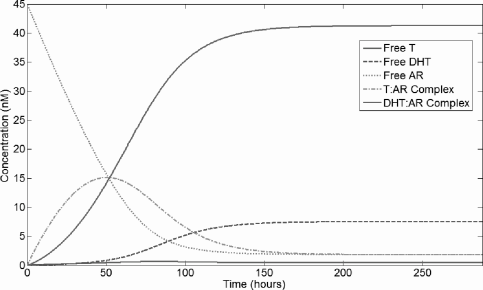
Time-series for the AR kinetics model. Free AR is set to 45 nM as an initial condition; all other variables are initially zero and baseline parameter values are used. Serum T is prescribed at 5 nM, inducing an influx of testosterone, and the model runs to a steady state.
5.5 Prostate growth mediated by androgens
We now link intracellular androgen concentrations to the proliferation and apoptosis of prostate epithelial cells. While we generally refer to low or high androgen levels causing a behavior, it is really the concentrations of AR:T and AR:DHT complexes that mediate these androgen-related activities. We introduce the variable Ct to represent the “effective” androgen:AR concentration. In [71], DHT was 2.4 times as potent as T in maintaining prostate weight and duct lumen mass, and these quantities varied linearly with either androgen. Therefore, we take Ct to be a simple linear combination of CT:R and CD:R:
Ct=CT:R+2.4CD:R. (5.48)
This approach allows the previously studied androgen kinetics model to be coupled directly to a model of prostate growth mediated by androgens. We let P(t) represent the number of prostate epithelial cells. We assume that the change in P is governed by two distinct death and proliferation signals; the per-capita proliferation rate is M(Ct, S) and the per-capita death rate is N(Ct, S), yielding the basic model framework:
dPdt=PM(Ct,S)−PN(Ct,S). (5.49)
We now determine the formal forms for M(Ct, S) and N(Ct, S). Prostate epithelial proliferation and death are regulated by androgens in several ways.
- Androgens induce stroma to produce factors, mainly bFGF and FGF-7, that support epithelial growth in a paracrine manner by supporting the prostate vasculature, induce epithelial proliferation, protect the epithelium from apoptosis, and regulate AR protein levels.
- Androgens may have a direct mitogenic effect upon epithelial cells through upregulation of proteins required for cell cycle progression.
- Androgens directly protect against apoptosis by negatively regulating TGF-β and increasing bcl-2 levels.
- Androgens mediate oxidative stress and the production of reactive oxygen species (ROS) within epithelial cells, which can induce proliferation, stasis, or death, depending upon the concentration.
Proliferation. It is generally accepted that androgens induce epithelial proliferation in vivo when the cell count is below normal, and androgen administration following castration induces rapid prostate regrowth in the rat [68, 70]. However, proliferation is thought to be limited, at least to some degree, by the homeostatic size of the prostate [46]. In our model, we assume that high levels of androgen directly induce proliferation while low levels cause apoptosis.
Redox state. The prostate redox state is also influenced by androgens, and this may be deeply important in epithelial death, proliferation, and carcino-genesis. Androgen blockade induces the production of ROS and subsequent oxidative stress. Several rat models have demonstrated that castration [62, 42] and treatment by either finasteride (5-α-reductase inhibitor) or flutamide (an anti-androgen) are strongly pro-oxidant [6]. Androgen withdrawal also causes vascular regression and prostate hypoxia [56], which in turn can induce ROS and increase expression of hypoxia inducible factor-1α (HIF-1α).
Androgen administration has also been shown to induce oxidative stress. Tam et al. [63] found that administration of testosterone with 17β-estradiol resulted in oxidative and nitrosative stress in the lateral lobe of the Noble rat. Ripple et al. [49] found that physiologic levels of DHT induced ROS in the LNCaP carcinoma cell line, and ROS generation preceded DHT induced proliferation.
Thus, a normal androgen environment likely promotes a balance between antioxidant and pro-oxidant activity [62], but both low and high androgen environments are pro-oxidant. Therefore, we assume that both low and high levels of androgen induce the formation of ROS.
ROS effects. At low levels, ROS act as important intracellular signalling molecules. A number of transcription factors, including NF-κB and AP-1 are redox sensitive, and modest levels of ROS are mitogenic. Higher levels of ROS can induce growth arrest and apoptosis, while very high levels can cause necrosis [10].
We assume that both low and high concentrations of Ct induce ROS and that there is some background level of ROS independent of androgens. We choose S to represent ROS and formally take
S=μ+θn1Cnt+θn1+CmtCmt+θm2. (5.50)
Here, µ is the background ROS level, and ROS is induced by low Ct and high Ct according to the first and second Hill functions, respectively. The half-maximal Ct for ROS induction by low androgen is θ1, while θ2 is the half-maximal Ct for high androgen induced ROS.
We assume that prostate proliferation is induced by increasing concentrations of such complexes, and a high cell count inhibits proliferation. Low AR:ligand complex concentration induces apoptosis, and there is always some small baseline turnover rate (1–2% of cells turnover daily in the healthy prostate [20]). Modest levels of ROS induce proliferation, while higher level cause growth arrest and apoptosis. These assumptions lead to our formal choices for M(Ct, S) and N(Ct, S):
M(Ct,S)=r2((C2tφ21+C2t)︸Androgen signal+ϕSe1−ϕS︸ROS signal)−σP︸crowding inhibition, (5.51)
N(Ct,S)=δ2((φ22C2t+φ22)︸Androgen signal+(Sqωq+Sq)︸ROS signal)+δ0︸normal turnover. (5.52)
Our incorporation of S as a function of Ct into the equation for dP/dt allows both direct and indirect ROS mediated effects of androgens on prostate growth to be incorporated into a single differential equation. This construction is somewhat similar to the ecological model of planktonic algae interaction with vegetation in shallow lakes proposed by Scheffer et al. [54].
The maximum per-capita proliferation rate is r, and the maximum death rate is δ + δ0. The direct proliferation signal due to androgens is modeled by a Hill function, with the strength of the signal increasing with Ct. The signal due to ROS is strong for low S and attenuates as S becomes large. Hill functions are used to model the death signals due to both androgen and ROS, with the signals strong for low Ct and high S, respectively. Cells also die at the background rate δ0, and the −σP term prevents unbounded growth.
The growth of the prostate epithelium in our model is governed solely by the intraprostatic weighted AR:ligand complex concentration, Ct, and the prostate cell count, P(t). There are two independent proliferation signals, one mediated by Ct and the other by S, and two similar death signals. The shapes of these signals are determined by the parameters θ1, θ2, φ1, φ2, ϕ, ω, n, m, and q.
Oxidative stress, S, is shown as a function of Ct in Figure 5.2. Figure 5.3 shows the proliferation and death signals due to Ct and S and their sums; these figures disregard the −σP crowding term as this always depends upon prostate size. The qualitative form of these curves is preserved over most of the parameter space.
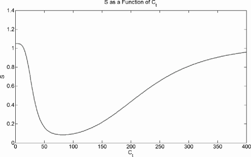
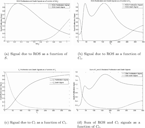
Curves for the different growth signals. Attenuation of proliferation by crowding is disregarded. Baseline parameter values are θ1 = 30 nM, θ2 = 225 nM, n = 4, m = 4, φ1 = 110 nM, φ2 = 40 nM, ϕ = 4, ω = 1, q = 8, σ = 1.5 × 10⁻¹⁰ cell−1 hour−1, 6 = 0.004 hour−1, r = ln(2)/24 hour−1, δ = ln(2)/24 hour−1.
5.6 Evolution and selection for elevated AR expression
In advanced cancers, upregulation of the AR protein is perhaps the single most important pathway by which cancers become hormone refractory. Chen et al. [8] found that in seven prostate cancer xenograft models, increased androgen receptor expression was the only change consistently associated with HR cancer progression. Rapid HR cancer recurrence in a xenograft model by Rocchi et al. was always associated with increased AR expression [51].
Because of the importance of the AR in prostate cancer progression, we investigate how different androgen environments select for cell lines expressing different levels of the AR; i.e., we examine selection upon Rt. To do this, we use the coupled AR kinetics and prostate growth model described in the previous section.
We have performed a series of numerical experiments where two or more epithelial cell strains, each having different values of Rt, compete with each other. Notably, these experiments suggest that selective pressure for increased AR expression varies with Rt and TS, but this nonuniform behavior makes it hard to gain insight using this simple approach. We suggest that implementing such a two-strain competition model numerically would be a useful exercise.
5.6.1 Model
To model competition between a large number of cell lines that evolve in time, Eikenberry et al. [14] proposed a state-transition model where cells transition between states that each represent a different level of Rt expression. We define a set of states
{Pi}Li=1. (5.53)
Each state represents a strain of prostate cells with a different AR concentration (i.e., Rt), and Rt varies linearly with i. Cells transition from Pi to Pi−1 and Pi+1 at rate γ, representing mutation. Populations of each strain grow according to the following coupled kinetics-growth model:
dPidt={PiM(Cti,Si)−PiN(Cti,Si)−2γPi+γPi−1+γPi+1,PiM(Cti,Si)−PiN(Cti,Si)−γPi+γPi+1,PiM(Cti,Si)−PiN(Cti,Si)−γPi+γPi−1,2≤i<L,i=1,i=L. (5.54)
We choose our model to have 100 states representing Rt from 15 to 114 nM. That is, we set L = 100 and Rti
5.6.2 Results
Figure 5.4 shows the evolution of average Rt under different serum T levels. In general, results indicate that physiologic serum T selects for increased AR expression, as do all androgen environments. Thus, the model predicts that even in healthy men, prostate epithelial cells will increase their potential for malignancy with time. Under high serum T, selection for an elevated Rt is actually slightly weaker. In comparison, low androgen environments (i.e., low serum T) demonstrate rapid, late selection for increased AR expression. While this selection occurs later in time, a higher average Rt is ultimately obtained.

Evolution of average Rt in the state-transition model under different serum T. AR expression is presumably a marker for the malignant potential of a strain. Low serum T selects for higher Rt than the normal environment (serum T = 5 nM), but takes longer to do so. High serum T selects for a slightly lower Rt.
We performed a sensitivity analysis to determine whether this behavior is preserved under other growth model parameter values. We found that the prediction that low androgen selects for a greater final Rt is always preserved. The parameters θ1, θ2, and µ, which govern the level of ROS, have the greatest effect on the dynamics. Overall, low androgen appears to select for a greater final Rt in all parameter space, but this selection becomes apparent later in time than under normal androgen for most parameter space.
These results suggest that a low androgen environment may delay the development of a malignant phenotype, but result in a more malignant or therapy-resistant strain later in time. This result could also be interpreted to mean that low androgen reduces the overall incidence of cancer, as the expected time to the development of a malignant strain is increased, but those cancers that do arise may be more aggressive. This notion is consistent with the results of finasteride treatment in men [64].
Having established one possible model framework by which the role of androgens in early cancer evolution may be studied, we now turn our attention to several models examining cancer recurrence driven by competition between androgen dependent (AD) and androgen independent (AI) cancer cell lines following androgen deprivation therapy (ADT). The focus of these models is evolution in a clinically meaningful, aggressive cancer, rather than long-term evolution predisposing cell lines toward malignancy.
5.7 Jackson ADT model
Jackson proposed a model [24, 25] describing the growth of a tumor spheroid consisting of two populations of cells—one that depends on androgen for survival and proliferation, and one that does not. Because the mathematical model is similar in form to that of Ideta et al. [23], discussed in the next section, we restrict our attention to some of Jackson’s key modeling assumptions: (1) the proliferation of androgen dependent (AD) cells increases in the presence of androgen, (2) the proliferation of androgen independent (AI) cells is unaffected by androgen levels, (3) the rate at which AD cells undergo apoptosis decreases in the presence of androgen, and (4) the rate at which AI cells undergo apoptosis increases in the presence of androgen. (As we discuss below, assumption (4) is debatable.)
In [24], Jackson predicted that androgen deprivation therapy would successfully control tumor growth for all time only in a small region in parameter space. This region is larger for total androgen blockade compared to partial androgen deprivation, but is still small. However, it is likely that this prediction is a consequence of the assumption that androgens harm AI cells. In [25], Jackson predicted that, following androgen ablation therapy, cancer could recur either through androgen-independent mechanisms such as upregulation of the anti-apoptotic protein bcl-2 in AI cells or through AR upregulation in AD cells. These two mechanisms corresponded to two qualitatively different patterns of recurrence, and the reader may consult the original paper for details.
The essence of the Jackson model is the tumor-wide balance between pro-liferation and death, which is expressed by the following ODE system:
dp(t)dt=αpθp(a)p−δpωp(a)p, (5.55)
dq(t)dt=αqθq(a)q−δqωq(a)q. (5.56)
Here, a is the concentration of androgen, assumed to be uniform throughout the tumor. Maximum per-capita growth rates are given by constants αp and αq, while constants δp and δq(a) represent the maximum per capita death rates for AD and AI cells, respectively. Parameters θp(a) ∈ [0, 1], θq(a) ∈ [0, 1], ωp(a) and ωq(a) mediate cell proliferation and death according to androgen levels.
Androgen-dependent cells are assumed to proliferate at rate αp in the presence of sufficient androgen. This rate decreases as androgen levels decrease, becoming θ1αp in the complete absence of androgen. AI cells always proliferate at the maximum rate αq. These assumptions can be satisfied by the following specific expressions:
θp(a)=θ1+(1−θ1)aa+K, (5.57)
θq(a)=1. (5.58)
Since 0 ≤ θ1 ≤ 1, then θp(0) = θ1 and θp(a) → 1 as a → ∞. The term a/(a + K) can be thought to represent saturation of a receptor governing the proliferative response to androgen.
Similarly, apoptosis rate in AD cells is assumed to be a decreasing function of androgen concentration. However, androgens are assumed to increase the the death rate of AI cells, which again is probably debatable. The functions ωp and ωq take on the same form as that used for θp:
ωp(a)=ω1+(1−ω1)aa+K,ω1>1, (5.59)
ωq(a)=ω2+(1−ω2)aa+K,0≤ω2≤1. (5.60)
We require ω1 > 1 to make ωp(a) a decreasing function of androgen. Also we have 0 ≤ ω2 ≤ 1, implying that ωq(a) decreases with increasing androgen. Parameters δp and δq represent the respective rates of apoptosis for AD and AI cells in a normal (high) androgen environment. As the androgen level approaches 0, the death rates go to ω1δp > δp and ω2δq < δq, respectively. Thus, ω1 and ω2 are the factors by which AD and AI cell death rates are modified in the complete absence of androgen.
To monitor the spatial distributions of the different cell types, one can keep track of the fluxes of the two classes of cancer cell, say Jp(r, t) and Jq(r, t). The net rate of collective cellular motion is determined by the balance between cell growth and death and the diffusive flux. The resulting partial differential equation model will have a moving tumor boundary. The rate of radial tumor expansion can also be tracked.
Jackson’s model considered both diffusive and advective fluxes. Diffusive flux is due to random cellular motion. Advective flux is often determined by some vector field. However, Jackson’s model “reverses” this—cells are not transported according to some vector field, but the net rate of collective cellular motion is given by the vector u, which is itself determined from the balance between cell growth and death and the diffusive flux. If we let p(r, t) and q(r, t) represent the tumor volume fraction of each class of cell (rather than some other metric such as absolute cell count), then Jackson’s model takes the form of the following conservation equations:
∂p∂t+∇⋅(up)=Dp∇2p+αpθp(a)p−δpωp(a)p, (5.61)
∂q∂t+∇⋅(uq)=Dq∇2q+αqθq(a)q−δqωq(a)q, (5.62)
Noting that p + q = k is constant, adding equations (5.61) to (5.62) yields the following expression for ∇⋅u
k∇⋅u=(Dp−Dq)∇2p+αpθp(a)p+αqθq(a)(k−p)−δpωp(a)p−δqωq(a)(k−p). (5.63)
Jackson assumes a spherically symmetric geometry, so the only component of the velocity is the radial component. This gives the rate of radial expansion for the tumor spheroid, which in turn allows tumor volume to be tracked. Using R(t) to represent the outer tumor radius, one arrives at an ODE for the rate of radial expansion, which is simply
dRdt=u(R(t),t). (5.64)
To complete the system, no flux boundary conditions are imposed at the inner (r = 0) and outer boundaries (r = R) of the spheroid. That is, at r = 0 and r = R
Dp∂p∂r(r,t)−u(R,t)p(r,t)=0,Dp∂p∂r(r,t)−u(R,t)p(r,t)=0. (5.65)
By symmetry, at r = 0,
∂p∂r(0,t)=∂q∂r(0,t)=0. (5.66)
These, together with no flux boundary condition at r = 0, yield
u(0,t)=0. (5.67)
The initial tumor radius is assumed to be R0 > 0, and cell conditions are uniform in space, with p(r, 0) = p0 and q(r, 0) = q0.
Finally, androgen levels are modified by treatment. Jackson considered two classes of treatment: castration through either surgical or chemical means (ADT); and total androgen deprivation (TAD), meaning castration in addition to anti-androgen drugs. The former reduces testosterone serum levels by up to 95%, but only reduces intraprostatic DHT by 50%, while the latter can reduce prostate DHT levels by 90% [20]. It is assumed that the androgen level, a(r, t), is at a steady-state until treatment is initiated at time T, at which point it declines exponentially to a new steady-state, either non-zero in the case of ADT or zero for TAB. Mathematically,
a(r,t)={a0;t<T,a0e−bt+as;t≥T, (5.68)
where as > 0 for ADT and identically 0 for TAB. We note that this model does not consider transitions between the cell classes, and the presence of androgen independent cells must be imposed in the initial conditions.
Jackson derived reasonable parameter values for growth and death rates of AD cells using biological data. Berges et al. [4] reported cell cycle times varying between 48 ± 5 hours for cancer cells. Based on this, a doubling time of 36 hours was assumed, still well within what is biologically reasonable (tumor cell doubling times typically vary between 1 and 4 days), yielding αp = αq = 0.4621 day−1. Using the data of Ellis et al. [15], the same data used to parameterize Swanson et al.’s PSA model [61], Jackson estimated δp = 0.3812, implying an overall growth rate of ρ = 0.0798 day−1. This is somewhat larger than Swanson et al.’s estimates. The parameter estimates for AI cells are more ad hoc. Table 5.5 shows all the parameters governing growth and death used by Jackson. No values or estimates for K, b, or as were published.
Parameter values for Jackson’s model, as reported in [24, 25].
Parameter |
Value |
|---|---|
αp |
0.4621 day−1 |
αq |
0.4621 day−1 |
δp |
0.3812 day−1 |
δq |
0.4765 day−1 |
θ1 |
0.8 |
ω1 |
1.18—1.35 |
ω2 |
0.25—1.0 |
p0 |
0.995 |
5.8 The Ideta et al. ADT model
Building on Jackson’s work, in 2008 Ideta et al. [23] proposed a model of intermittent androgen deprivation therapy and evolution toward androgen-independent cancer recurrence. Like Jackson’s, this model considers androgen levels, represented by a(t), androgen-dependent cells, x1(t), and androgen-independent cells, x2(t). Androgen levels approach some homeostatic set-point that can be modified by androgen deprivation therapy (ADT). Androgen-mediated growth and death reflect Jackson’s assumptions, but three different hypotheses concerning how androgens affect AI cell proliferation are considered:
- Normal androgen levels have no effect on AI cell proliferation.
- AI cell proliferation is negatively regulated by androgens, and at a defined normal androgen level (a0) proliferation and apoptosis completely balance each other, giving a net growth rate of zero.
- AI proliferation is negatively regulated by androgen, and the net growth rate is negative at the normal androgen level.
Androgen-dependent cells mutate to become AI cells at a rate that increases with decreasing androgen levels. This assumption apparently stems from the notion that low androgen induces transformation into an androgen-independent phenotype. These considerations yield the following model:
dadt=−γa+γa0(1−u), (5.69)
dx1dt=α1p1(a)x1−β1q1(a)x1−m(a)x1, (5.70)
dx2dt=α2p2(a)x2−β2q2(a)x2+m(a)x1, (5.71)
where, like in Jackson’s model,
p1(a)=k1+(1−k1)aa+k2,0≤k1≤1, (5.72)
q1(a)=k3+(1−k3)aa+k4,k3≥1, (5.73)
p2(a)={1;for hypothesis (1),1−(1−β2α2)aa0;for hypothesis (2),1−aa0;for hypothesis (3), (5.74)
q2(a)=1, (5.75)
m(a)=m1(1−aa0). (5.76)
Treatment is represented by the effect of u, which is either 1 (treatment on) or 0 (treatment off). Similar to Jackson’s model, AD cells proliferate at the baseline rate α1k1. As a → ∞, this rate approaches α1 as the proliferative response saturates. For k3 > 1, q1(a) causes the death rate to increase with decreasing androgen, equaling β1k3 when a = 0. The Ideta et al. model departs from Jackson’s in considering three hypotheses for AI proliferation in response to androgen and in assuming a constant AI apoptosis rate regardless of androgen concentration (q2(a) ≡ 1).
The rate of transition from AD to AI cells decreases linearly from m1 at a = 0 to 0 when androgen concentration is normal; i.e., a = a0. As discussed previously, this is controversial. The dependence on a0 in many of the functions causes AI proliferation to become negative if a > a0 for hypotheses (2) and (3), while m(a) also becomes negative, implying that AI cells begin transitioning into AD cells in a high androgen environment.
Ideta et al. proposed an algorithm for governing treatment in which androgen deprivation is turned on or off depending on the level of system androgen and the rate of change in tumor growth. It is assumed that, clinically, only the serum PSA level can be tracked, rather than the actual tumor volume. Represented by y(t), PSA concentration is assumed to be a simple function of AD and AI cells with no lag in production; therefore,
y(t)=c1x1(t)+c2x2(t). (5.77)
This equation is the same fundamental relationship that we studied earlier in the context of PSA dynamics (see equation (5.4)). Ideta et al. set c1 = c2 = 1, implying that PSA tracks tumor growth precisely. In our earlier exploration of PSA dynamical models, we determined that the PSA level in individuals correlates poorly with absolute tumor volume, but likely tracks relative changes in tumor volume quite well. Thus, we suggest that this assumption is only a reasonable initial approximation.
The algorithm for cycling treatment turns treatment on when PSA is both sufficiently high and increasing, turns it off when PSA is both sufficiently low and decreasing; this is formally modeled as follows:
u(t)={0→1when y(t)=r1 and dy/dt>0,1→0when y(t)=r0 and dy/dt<0, (5.78)
where r1 is the threshold PSA for activating treatment, and r0 is the threshold PSA for ceasing treatment.
Ideta et al. examined the efficacy of cycling androgen deprivation therapy under the three hypotheses for the growth of AI cells in an androgen rich environment. Importantly, they found that only under hypotheses (2) and (3), where androgens inhibit AI cell proliferation, does intermittent therapy delay androgen-independent relapse. Since we have argued on biological grounds that these hypotheses are unlikely in an in vivo tumor, or at most account for only a small fraction of AI tumors, the results under hypothesis (1) are the most clinically relevant.
Figure 5.5 shows how different schedules of intermittent therapy (i.e., different r0s) affect time to AI relapse. Under hypothesis (3), any treatment cycling at all permanently prevents relapse, while continuous androgen deprivation results in aggressive recurrence. Under hypothesis (2), relapse is only delayed by intermittent therapy, while under hypothesis (1), intermittent therapy slightly reduces the time to relapse. However, because it can reduce the side effects of therapy and improve quality of life, a slightly shorter time to relapse may be an acceptable trade-off.
![Figure showing Intermittent androgen deprivation therapy in Ideta et al.’s model [23] under the three hypotheses for the effect of androgens on AI cell proliferation. Parameter values are α1 = 0.0204 (bone mets) to 0.0290 (lymph node mets), α2 = 0.0242 to 0.0277, β1 = 0.0076 to 0.0085, β2 = 0.0168 to 0.0222, k1 = 0, k2 = 2, k3 = 8, k4 = 0.5, γ = 0.08, a0 = 30, and m1 = 0.00005 to 0.0002.](http://imgdetail.ebookreading.net/math_science_engineering/24/9781498785532/9781498785532__introduction-to-mathematical__9781498785532__image__fig5-5.png)
Intermittent androgen deprivation therapy in Ideta et al.’s model [23] under the three hypotheses for the effect of androgens on AI cell proliferation. Parameter values are α1 = 0.0204 (bone mets) to 0.0290 (lymph node mets), α2 = 0.0242 to 0.0277, β1 = 0.0076 to 0.0085, β2 = 0.0168 to 0.0222, k1 = 0, k2 = 2, k3 = 8, k4 = 0.5, γ = 0.08, a0 = 30, and m1 = 0.00005 to 0.0002.
Interestingly, the Ideta et al. treatment algorithm suggests that modifying the one governing parameter, r0, can greatly affect the time to relapse, with a lower r0 significantly increasing the time to relapse. As can be seen from Figure 5.5, a lower r0 roughly translates to a longer period of treatment cycling. Moreover, the simplicity of this algorithm makes its clinical use feasible.
5.9 Predictions and limitations of current ADT models
Both the Jackson and Ideta et al. model formulations assume that AI cells are either out-competed or do not arise in normal androgen environments. As the authors note, this assumption is reasonably justified from the biological observation that such cells are not routinely observed in untreated prostate cancers. It remains an open question, however, how selection operates on AI cells in an androgen-rich environment. It is certainly possible that selection disfavors AI cells in such an environment. Alternatively, the AI phenotype may be neutral—neither favored by selection nor disfavored. In the latter case, one could expect at least a small population of AI cells to exist in prostate cancers before androgen ablation begins. In a few cases, the population may become quite sizable prior to androgen ablation, since neutral traits can spread through populations by genetic drift.
The Jackson model specifically hypothesizes that selection acts against androgen-independent clones in environments with high androgen concentrations. There is some evidence, primarily from in vitro cell line data, that in some cases physiologic androgen levels can induce apoptosis in androgen independent prostate cancer cells. However, administration of androgens in hormone-refractory cancer nearly always results in disease flare [20]. Furthermore, AI cells generally retain some dependence upon the AR and usually evolve to a so-called androgen independent state by activating AR dependent genes through other means. These observations support the alternative hypothesis that androgens promote proliferation in both AI and AD cells. The degree to which this assumption affects the dynamics and predictions of Jack-son’s model is unclear. If this alternative hypothesis were true, then the Ideta et al. model would also be affected since it explores the possibilities of androgen having either no effect on AI cell growth or a negative effect. However, the Ideta et al. model could be extended to explore this possibility and its effects on treatment cycling.
These models highlight the difficulty of examining evolutionary dynamics when competition between a limited number of pre-defined clones is considered. However, despite their limitations, the Jackson and Ideta et al. models do make several interesting predictions. Specifically, they predict that only a small region of parameter space will allow androgen ablation therapy to completely control prostate cancer. Furthermore, in the case of AI cells whose growth is inhibited by androgens, intermittent androgen deprivation can delay or prevent AI relapse. If the proliferation of AI cells is unaffected by androgens, then intermittent therapy can slightly reduce the time to relapse. Also, more infrequent cycling of therapy delays relapse.
5.10 An immunotherapy model for advanced prostate cancer
Cancer immunotherapy has been studied with a mathematical model by Kirschner and Panetta [29]. Their model examines the dynamics between the adaptive immune system, tumor cells, and the cytokine interleukin-2 (IL-2). The model shows that the immune system can control tumors with average to high antigenicity at a dormant state. However, their results suggest that treatment with IL-2 alone may not clear the tumor without administering toxic levels of the cytokine. Partially motivated by the work of Kirschner and Panetta [29], Porta and Kuang [44] formulated a mathematical model of advanced prostate cancer treatment to examine the combined effects of ADT and immunotherapy.
From previous sections we know that ADT, while initially successful, eventually results in a relapse after two to three years in the form of androgen-independent prostate cancer. Intermittent androgen deprivation therapy attempts to enhance quality of life and occasionally prevent relapse by cycling the patient on and off treatment. Over the past decade, dendritic cell (DC) vaccines have been used with some success in clinical studies for the im-munotherapy of prostate cancer. Although these studies found that the DC vaccines could slow the progression of the disease in hormone refractory patients, they did not show how the vaccine would affect patients actively undergoing hormone therapy.
In this section we present the Portz-Kuang model, which studies the efficacy of dendritic cell vaccines when used with continuous or intermittent ADT schedules. Their model may determine if intermittent therapy has any benefits over continuous therapy, other than improved quality of life, when combined with the use of DC vaccines. The necessary conditions for disease elimination or stabilization using such combined treatments can also be examined by this model. Numerical simulations of the Portz-Kuang model suggest that immunotherapy can indeed successfully stabilize the disease using both continuous and intermittent androgen deprivation. This section is adapted from the work contained in Portz and Kuang [44].
In Portz and Kuang [44], the prostate cancer treatment by immunother-apy and androgen deprivation therapy is modeled by a system of ordinary differential equations which takes the form,
dX1dt=r1(A)X1︸proliferation and death−m(A)X1︸mutation to AI−e1X1Tg1+X1︸killed by T cells, (5.79)
dX2dt=r2X2︸proliferation and death+m(A)X1︸mutation from AD−e1X2Tg1+X2︸killed by T cells, (5.80)
dTdt=e2Dg2+D︸activation by dendritic cells−μT︸natural death+e3TILg3+IL︸clonal expansion, (5.81)
dILdt=e4T(X1+X2)g4+X1+X2︸production by stimulated T cells−ωIL︸clearance, (5.82)
dAdt=γ(a0−A)︸homeostasis−γa0u(t)︸deprivation therapy, (5.83)
dDdt=−cD︸natural death. (5.84)
The variables used in the model and their meanings are listed in Table 5.6. Parameter interpretations and estimates are given in Table 5.7.
Variables in the Portz-Kuang model.
Variable |
Meaning |
Unit |
|---|---|---|
X1 |
number of androgen-dependent cancer cells |
cells |
X2 |
number of androgen-independent cancer cells |
cells |
T |
number of activated T cells |
cells |
IL |
concentration of cytokines |
ng/ml |
A |
concentration of androgen |
nmol/ml |
D |
number of dendritic cells |
cells |
Parameters (Para.) in the Portz-Kuang model.
Para. |
Meaning |
Value |
Ref. |
|---|---|---|---|
α1 |
AD cell proliferation rate |
0.025/day |
[4] |
β1 |
AD cell death rate |
0.008/day |
[4] |
k1 |
k1 AD cell proliferation rate depen-dence on androgen |
2 ng/ml |
[23] |
k2 |
effect of low androgen level on AD cell death rate |
8 |
[5] |
k3 |
AD cell death rate dependence on androgen |
0.5 ng/ml |
[23] |
r2 |
AI cell net growth rate |
0.006/day |
[4] |
m1 |
maximum mutation rate |
0.00005/day |
[23] |
a0 |
normal androgen concentration |
30 ng/ml |
[23] |
γ |
γ androgen clearance and produc-tion rate |
0.08/day |
[23] |
ω |
cytokine clearance rate |
10/day |
[52] |
μ |
T cell death rate |
0.03/day |
[29] |
c |
dendritic cell death rate |
0.14/day |
[35] |
e1 |
e1 maximum rate T cells kill cancer cells |
0 − 1/day |
[29] |
g1 |
cancer cell saturation level for T cell kill rate |
10 × 109 cells |
[29] |
e2 |
maximum T cell activation rate |
20 × 106 cells/day |
[29] |
g2 |
DC saturation level for T cell ac-tivation |
400 × 106 cells |
[57] |
e3 |
e3 maximum rate of clonal expan-sion |
0.1245/day |
[29] |
g3 |
IL-2 saturation level for T cell clonal expansion |
1000 ng/ml |
[29] |
e4 |
e4 maximum rate T cells produce IL-2 |
5 x 10⁻⁶ ng/ml/cell/day |
[29] |
g4 |
cancer cell saturation level for T cell stimulation |
10 × 109 cells |
[29] |
D1 |
DC vaccine dosage |
300 × 106 cells |
[57] |
c1 |
AD cell PSA level correlation |
10−9 ng/ml/cell |
[23] |
c2 |
AI cell PSA level correlation |
10−9 ng/ml/cell |
[23] |
As in the previous section, the androgen-dependent functions for AD cell growth and mutation are defined as follows:
r1(A)=α1AA+k1−β1(k2+(1−k2)AA+k3), (5.85)
m(A)=m1(1−Aa0). (5.86)
The parameters in the expression for r1(A) are chosen such that the net growth rate of AD cells is α1 − β1 when A = a0 or −β1k2 when A = 0. The value of parameter k2 is chosen such that β1k2 matches the rate of decline of serum PSA concentration during continuous ADT [23]. The net growth rate of AI cells, r2, is a constant in this version of the model. Ideta et al. proposed two alternatives for r2 which assumed that androgen had a negative effect on the proliferation rate of AI cells [23]. Mutation from AD to AI occurs at a rate m1 when A = 0, and no mutation occurs when A = a0. Larger values of m1 result in a shorter time to androgen-independent relapse; thus, relapse time can be used to estimate the value of m1 [23].
Intermittent androgen deprivation therapy is modeled by equation (5.83) where u(t) = 0 indicates an on-treatment period, and u(t) = 1 indicates an off-treatment episode. During off-treatment periods, the androgen level tends toward the set-point androgen level, a0. Androgen decays at a rate γ during on-treatment periods. The treatment function, u(t), is controlled by monitoring the serum PSA level as we saw earlier:
y(t)=c1X1+c2X2, (5.87)
u(t)={0→1 when y(t)>L1 and dy/dt>0,1→0 when y(t)<L0 and dy/dt<0, (5.88)
where y(t) is the serum PSA concentration. Androgen deprivation is switched on when the serum PSA concentration exceeds some level, L1, and switched off when the serum PSA concentration drops below some level, L0, with L0 < L1.
Since T cells are activated and stimulated through interactions between proteins (antigens and cytokines) and receptors [31], Michaelis-Menten kinetics are used for all immune response terms in the model. This is the approach taken by Kirschner and Panetta and is reasonable given that high levels of antigens and cytokines are likely to have a saturation effect on the T cells. IL-2 is included in the model to provide the clonal expansion dynamics of helper T cells. When stimulated by the antigens presented on tumor cells, the helper T cells produce IL-2. The IL-2 then stimulates the clonal expansion of T cells in a positive feedback loop [31]. The model assumes a constant ratio of cytotoxic and helper T cells, which greatly simplifies the model and should not have a significant impact on the long-term behavior of the system. The cytotoxic T cells interact with and kill the tumor cells based on antigen stimulation. The rate of interaction is assumed to be the same for both AD and AI cells. There is no biological reason to assume otherwise.
The antigen-loaded dendritic cells are modeled by equation (5.84), which assumes that the DCs undergo apoptosis at a constant rate and are not being replenished by any mechanisms other than further vaccinations. Vaccinations are administered every 30 days in model simulations. Each vaccination contains D1 antigen-loaded DCs. The DCs are assumed to activate naïve T cells based on Michaelis-Menten kinetics, as shown in (5.81). The model assumes that there are always naïve T cells available for activation.
The Michaelis-Menten terms could be replaced by simpler mass action terms to make the non-zero steady states easier to find analytically. However, the system is repeatedly being perturbed by the administration of DC vaccines, so steady-state analysis has limited use. For this and several other reasons, the model was analyzed primarily through numerical simulations in Portz and Kuang [44] with Michaelis-Menten terms.
When a dendritic cell vaccine is combined with continuous androgen deprivation, the model shows that the cancer can be eliminated with a relatively strong (but still within a reasonable parameter range) antitumor immune response. Clinical studies have shown that DC vaccines are able to stabilize disease progression in some patients with hormone refractory prostate cancer. Since these patients have androgen-independent cancer, we can safely assume that DC vaccines are capable of stopping the net growth of AI cells. When administered to a patient actively undergoing hormone therapy, one would expect the DC vaccine to prevent an androgen-independent relapse while allowing continuous androgen deprivation therapy to eliminate the AD cell population. Thus the results of the above model are reasonable in the case of DC vaccination combined with continuous androgen deprivation.
An interesting result of the model is that the DC vaccine is able to prevent relapse with a slightly weaker antitumor immune response when intermittent androgen deprivation is used instead of continuous androgen deprivation. While the difference was only small (e1 = 0.68973 compared to e1 = 0.69197), the result was still surprising considering the effect that intermittent therapy has on relapse time without immunotherapy. This small difference can likely be attributed to the ability of the immune response to offset the higher mutation rate when intermittent therapy is used and also to the consistently larger cancer cell population which is necessary to stimulate the clonal expansion of T cells. With the low toxicity of DC vaccines [57] and the quality-of-life benefits of IAD, the combination of these two treatments could be very advantageous over continuous ADT for the treatment of advanced prostate cancer.
The hybrid nature of the model—combing continuous treatment dynamics with discrete treatment—makes standard analysis difficult. This situation forced Portz and Kuang [44] to use specific parameter values to find the desired values of e1, preventing the possibility of having an algebraic expression for those values of e1. Simplifying the model may be possible by using some simple continuous functions for the D(t) and u(t), although it would likely make clinical application of the model infeasible.
Accuracy in the estimation of parameter values for the immune response is a significant limitation of the model. Most of the parameter estimates were based on those used by Kirschner and Panetta [29]. While many of these parameter estimates were based on data from biological studies, the estimates are for generic antitumor immune responses. The proper parameter values for an immune response against prostate cancer may be significantly different.
Another serious limitation of the model is the lack of regulatory T cells, which reduce sensitivity to self-antigens and prevent self-destructive lymphocyte responses [41]. Since targeting cancer cells requires targeting self-antigens, regulatory T cells may have a significant suppressive effect on antitumor immunity [72]. Several studies have examined ways to target regulatory T cells to reduce their suppressive effect on immunotherapy [72]. Including regulatory T cells in the model is a possible direction for future work, and the therapies which target the regulatory T cells could then be examined.
5.11 Other prostate models
While we have primarily restricted our focus to prostate cancer, we would be remiss if we did not mention the model of Barton and Anderson [3] and its extension by Potter et al. [45] on androgen regulation of prostate growth. It is a complicated, compartmentalized pharmacokinetics model that comprehensively describes androgen dynamics and may serve as a valuable resource in developing future models more focused on cancer dynamics.
Jain et al. [26] formulated a comprehensive mathematical model of prostate cancer progression in response to androgen ablation therapy based on the model framework described in this chapter, which is adapted from the work presented in [14]. Their model includes patient-dependent parameters and captures a variety of clinically observed outcomes for typical patient data under various intermittent schedules. They fit their simulations to data reported in the literature, and then project the future course of the disease for the next 5 to 10-year period under either intermittent or continuous therapy. Their model predicts that intermittent scheduling will yield more benefit if hormone-sensitive cells have a competitive advantage since it may delay the acquisition of genetic or epigenetic alterations empowering androgen resistance. Subsequently, Jain and Friedman [27] presented some simplifications and variations to the model and carried out systematic computational and mathematical analysis of their simplified models. Most noteworthy is their novel mathematical definitions of treatment viability, treatment failure and treatment failure time. These rigorous definitions enable the authors to effectively compare and contrast prostate cancer response to continuous versus intermittent androgen ablation therapy via mathematical models. Friedman and Jain [16] also formulated and studied a free boundary partial differential equation model of metastasized prostatic cancer where they were able to establish the existence and uniqueness of solution for the model. In addition, they also established the global existence of solutions for the radially symmetric case.
Dimonte, an advanced stage prostate cancer patient and an experienced mathematical modeler, developed a sophisticated cell kinetics model for prostate cancer progression from diagnosis to final clinical outcome subject to various treatment strategies [11]. To describe hormone ablation therapy, Di-monte assumed the existence of three cancer cell populations: (1) cells local to the prostate and sensitive to hormones, (2) regional and hormone sensitive cells, and (3) systemic and hormone resistant cells. The model comprises three coupled first-order differential equations, each describing dynamics of one of these three populations. Time is scaled to the doubling time of the prostate specific antigen concentration. The rate at which local cells transition to the systemic compartment is associated with the patient’s Gleason score. The model also assumes three threshold cell population sizes that represent (1) initiation of tumor spread out of the local compartment, (2) saturation capacity of the local tumor, and (3) the cell count likely to cause PC-specific death. These parameters can be calibrated using published PC clinical data and survival tables. Dimonte then applies the model to two individuals (himself and another) with complete PC diagnostic data and calculates the time to PC-specific death. In a subsequent model, Dimonte et al. [12] introduced a simplification and employed it to clarify the observed variability among biochemical recurrence nomograms for prostate cancer and suggested that nomograms should be stratified by PSA doubling time to improve predictive power.
In the same issue of the journal published the work of Dimonte [11], Hirata et al. [22] introduced a mathematical model for serum PSA dynamics in patients receiving intermittent androgen suppression (IAS) for prostate cancer. The validity of their model is supported by patient data obtained from a clinical trial of IAS. More specifically, Hirata et al. [21] formulated an intermittent androgen ablation model that comprises two submodels: an on-treatment linear model; and an off-treatment linear model. Their model considered an AD cell population (x1), a reversible AI cell population (x2), and an irreversible AI cell population (x3), modeled by the following linear system
ddt(x1(t)x2(t)x3(t))=(w11,100w12,1w12,20w13,1w13,20)(x1(t)x2(t)x3(t)) (5.89)
for the on-treatment periods, and
ddt(x1(t)x2(t)x3(t))=(w01,1w01,200w12,2000w03,3)(x1(t)x2(t)x3(t)) (5.90)
for the off-treatment periods. Hirata et al. constrained the parameters so that all those off the diagonal are non-negative, while w03,3>0
In contrast, a more mechanistic model of intermittent androgen ablation treatment was formulated by Portz et al. [43]. This model uses androgen and PSA data from individual patients to calibrate the various model parameters, which are clinically measurable or can be estimated from data in literature. Their model fits multiple cycles of individual patient PSA data very well, with parameter values obtained from the data well within observed physiological ranges. We will cover their model and its variations in some detail in the next chapter.
5.12 Exercises
Exercise 5.1: Systematically study the global dynamics of the ODE version of Jack-son’s model, consisting of equations (5.55)–(5.56), with three different treatment scenarios as described by the following androgen profiles.
a(t)={a0;t< T,for no treatment,a0e−bt+as;t≥T,for ADT,a0e−bt;t≥T,for TAB therapy. (5.91)
Exercise 5.2: Reproduce the Figure 3 in [24].
Exercise 5.3: Systematically study the global dynamics of the Ideta et al. model under hypothesis (1) (i.e., p2(a) ≡ 1). Show that intermittent ADT reduces time to relapse as illustrated by the Figure 5.5. In other words, continuous ADT is slightly superior in terms of delaying treatment resistance.
Exercise 5.4: Systematically study the global dynamics of the Ideta et al. model under hypothesis (2) (i.e., p2(a) ≡ 1). Show that intermittent ADT increases time to relapse as illustrated by the Figure 5.5. In other words, both intermittent and continuous ADT will result in treatment resistance, with intermittent ADT being superior in delaying treatment resistance.
Exercise 5.5: Systematically study the global dynamics of the Ideta et al.’s model under hypothesis (3) (i.e., p2(a) ≡ 1). Show that any treatment cycling at all permanently prevents relapse as illustrated by the Figure 5.5.
Exercise 5.6: In a recent paper by Jain and Friedman [27], the authors formulated a model for prostate carcinoma growth and treatment with androgen deprivation therapy. The principal species modeled are the following: number of androgen-dependent cancer cells in millions (N), number of castration-resistant cancer cells in millions (M), and serum PSA concentration in ng/ml (P). When treatment is off (u(t) = 0), N and M grow at rates αN(1 − ∊M)N and αmM + αN ∊m N, respectively, and have growth rates −βNN and βM M, respectively, when the treatment is on. Jain and Friedman assume that androgen-dependent cells mutate irreversibly to an androgen-independent phenotype with probability ∊M. Both androgen-dependent and -independent cells are assumed to produce PSA. These assumptions yield the following model:
dNdt=αN(1−∈M)N(1−u(t))−βNNu(t), (5.92)
dMdt=(αMM+αN∈MN)(1−u(t))+βMMu(t), (5.93)
dPdt=θNN+θMM−λPP. (5.94)
Solve the above system explicitly in cases when the treatment is locked on and locked off.
Exercise 5.7: Reproduce Figure 4 in the paper by Jain and Friedman [27].
Exercise 5.8: Simulate the model of Portz and Kuang [44] with parameters given in Table 5.7. You may use or adapt the following MATLAB® program.
-----------------------------------------------------------
% MATLAB program to simulate a prostate cancer model with intermittent
% ADT and dendritic cell vaccine immunotherapy
tstart = 0; tfinal = 1200;
x0=[15;0.1;0;0;30;0]; % initial conditions (billions of cells)
% treatment parameters
u = 1; % androgen-ablation on/off state
L0 = 3; % androgen-ablation off PSA value
L1 = 13; % androgen-ablation on PSA value
%D1 = 0.3; % number of DCs (billions) in single infusion
D1 = 0;
tstep = 1200;
%tstep = 30; % days between immunotherapy injections
% tumor size to PSA level correlation parameters
c1 = 1; c2 = c1;
tout = tstart; xout = x0.’;
teout = []; xeout = []; ieout = [];
options = odeset(’Events’, @(t,x)events(t,x,c1,c2,L0,L1,u));
first = true;
tprev = tstart;
while tstart < tfinal
[t,x,te,xe,ie] = ode45(@(t,x)f(t,x,u),...
[tstart min([tprev+tstep tfinal])],x0,options);
nt = length(t);
tout = [tout; t(2:nt)];
xout = [xout; x(2:nt,:)];
if isempty(ie)
% administer DC vaccine
D = x(nt,6)+D1;
tprev = t(nt);
else
% toggle androgen ablation therapy
u = 1 - u;
D = x(nt,6);
end
% adjust initial conditions
x0 = x(nt,1:5);
x0(6) = D;
options = odeset(’Events’, @(t,x)events(t,x,c1,c2,L0,L1,u),...
’InitialStep’,t(nt)-t(nt-1),’MaxStep’,t(nt)-t(1));
tstart = t(nt);
end
!
y = c1.*xout(:,1) + c2.*xout(:,2);
Figure(1);
hold off
plot(tout,y,’k’,’LineWidth’,1.5);
xlabel(’time (days)’); ylabel(’PSA (ng/mL)’);
set(gca,’xlim’,[0 tfinal],’ylim’,[0 40]);
box on
Figure(2);
hold off
plot(tout,xout(:,5),’k-’,’LineWidth’,1.5);
xlabel(’time (days)’);
ylabel(’Androgen (nmol/L)’);
set(gca,’xlim’,[0 tfinal],’ylim’,[0 40]);
box on
Figure(3);
hold off
subplot(2,1,1);
plot(tout,xout(:,1),’k’,’LineWidth’,1.5);
xlabel(’time (days)’); ylabel(’AD cells’);
subplot(2,1,2);
plot(tout,xout(:,2),’k-’,’LineWidth’,1.5);
xlabel(’time (days)’); ylabel(’AI cells’);
% --------------------------------------------------------------
function dxdt = f(t,x,u)
X1 = x(1); X2 = x(2); T = x(3); IL = x(4); A = x(5); D = x(6);
alpha1 = 0.025; beta1 = 0.008;
k1 = 2; k2 = 8; k3 = 0.5; alpha2 = 0.025; beta2 = 0.019;
m1 = 0.00005; % mutation rate
a0 = 30; % normal androgen level
gamma = 0.08; % androgen clearance rate
c = 0.14; % DC death rate
e1 = 0.6897325;
g1 = 10; e2 = e1; g2 = g1;
e3 = 0.02; % T-cell sensitivity to dendritic cells
g3 = 0.4;
e4 = 0.1245; % T-cell sensitivity to IL-2
g4 = 1e3;
e5 = 5e3; % IL-2 production from T cell stimulation
g5 = 10;
mu = 0.03; % T-cell death rate
omega = 10; % IL-2 clearance rate
r1 = alpha1*A/(A+k1) - beta1*(k2+(1-k2)*A/(A+k3));
r2 = alpha2 - beta2;
m = m1*(1-A/a0);
dX1 = r1*X1 - m*X1 - e1*X1*T/(g1+X1);
dX2 = r2*X2 + m*X1 - e2*X2*T/(g2+X2);
dT = e3*D/(g3+D) - mu*T + e4*T*IL/(g4+IL);
dIL = e5*T*(X1+X2)/(g5+X1+X2) - omega*IL;
dA = gamma*(a0-A)-gamma*a0*u;
dD = -c*D;
dxdt = [dX1; dX2; dT; dIL; dA; dD];
% --------------------------------------------------------------
function [value,isterminal,direction] = events(t,x,c1,c2,L0,L1,u)
% hysteresis relay
isterminal = 1;
if u == 1
value = c1*x(1) + c2*x(2) - L0;
direction = -1;
else
value = c1*x(1) + c2*x(2) - L1;
direction = 1;
end
-----------------------------------------------------------
Exercise 5.9: Consider a special case of the model in Portz and Kuang [44] in which there is just one type of tumor cells X1. This can be achieved by assuming X2(0) = 0 and m(A) = 0. Assume also that both the dendritic cell density and the androgen level are constant so that their model is reduced to a system of just three equations. In addition, assume that the term describing T-cells killing cancer cells can be modeled by a mass action term and same for the term describing the IL-2 production due to T-cell stimulation. Study the boundedness of solutions, existence of steady states and the stability of the steady states of this reduced system.
Exercise 5.10: In addition to the assumptions presented in the previous exercise, apply a quasi-steady state approximation on the IL-2 equation. This shall reduce the model to a system of two equations. Study the boundedness of solutions, existence of steady states, the local and global stability of the steady states of this dramatically reduced system.
5.13 Projects
Here, we briefly suggest some modifications or extensions of existing dynamical models that could be pursued as meaningful projects by the interested students.
5.13.1 The epithelial-vascular interface and serum PSA
A surprising and important prediction of Vollmer and Humphrey’s model is that at steady state the serum PSA does not depend upon β, the rate of transport from the interstitium to the serum, which is a marker for the extent of the epithelial-vascular interface. Moreover, we have found that when PSA is increasing according to an empirical exponential model, β has a minimal effect on PSA over most biologically reasonable parameter space. It is important to determine if this prediction is robust under different model constructions. For example, one can model transport as a function of the vascular surface area, A, the PSA concentration difference in the tissue and serum compartments, (f − y), and a permeability coefficient P. This gives the new model,
dfdt=α−PA(f−y)1Vp, (5.95)
dydt=PA(f−y)1Vs−ky. (5.96)
Some simple calculations show that the steady state for this model is
fs=αVpPA+αVpkVs, (5.97)
ys=αVpkVs, (5.98)
Thus, while the tissue PSA steady state is more complex and explicitly depends on the transport parameters P and A, serum PSA is unchanged from the original model, remaining independent of the vasculature. An important advantage of this formulation is that the parameters P and A may be estimated directly from empirical biological data.
We now return to the original model, but suggest that the PSA in the tissue compartment should also degrade at some rate µ. This yields another modified model:
dfdt=α−βf−μf, (5.99)
dydt=βf−ky. (5.100)
fs=αβ+μ, (5.101)
ys=αβk(β+μ)VpVs. (5.102)
Thus, PSA degradation in the tissue compartment causes steady state serum PSA to depend upon β, and therefore the epithelial-vascular interface. We suggest that the interested student more thoroughly examine and characterize the dynamics of these modified models, and as a final modification, combine the two. This would allow a more detailed understanding of how tissue compartment PSA dynamics and transport parameters interact to determine serum PSA, hopefully giving deeper insight into the importance of the tissue-vascular interface in determining serum PSA.
5.13.2 A clinical algorithm based on a dynamical model
Our analysis of the models of both Swanson et al. [61] and Vollmer and Humphrey [67], among other things, suggests that serum PSA is not a reliable predictor of tumor volume in individual cases. Indeed, serum PSA in the 4 to 10 ng/ml range is not a reliable predictor of the presence of clinically meaningful cancer. Therefore, in order to determine if an individual patient’s PSA indicates the existence of cancer, we propose the following example algorithm:
- Assume cancer does not exist.
- Use several serial PSA measurements to determine PSA velocity.
- Measure prostate volume by transrectal ultrasound and estimate epithelial fraction.
- Calculate the likely range of serum PSA under equation (5.25) derived by Vollmer and Humphrey [67] (but with Vc = 0).
In other words, we are deriving a PSA interval implied by a null hypothesis— viz. that cancer is not present—based on several individually measured parameter values and the normal value range for the other parameters. If the PSA is outside the range predicted by the null hypothesis, then we may accept the alternative hypothesis that cancer is present. An algorithm along these lines, tested on a clinical data-set, could be of clinical use.
5.13.3 An extension of Vollmer and Humphrey’s model
As it stands, γ, the relative PSA velocity, reflects the growth of both benign and cancerous tissues. Both c1 and c2 are affected by γ. One could productively extend Vollmer and Humphrey’s model by adding an explicit model of tumor growth. A simple exponential growth model could be used as a first approximation; e.g.,
Vc=V0eγt. (5.103)
Total prostate volume,
Vp=Vb+Vc, (5.104)
would cease to be constant. Further analysis of this or a similar model could give a better understanding of the relative contribution to PSA change by cancerous tissue compared to benign tissue. Growth in the benign tissue compartment could also be considered explicitly.
5.13.4 Androgens positively regulating AI cell proliferation
In the model of Ideta et al. [23], we can assume that androgens increase AI proliferation, and even in the absence of androgens there is some small but positive proliferation rate. Therefore, AI cells will have a proliferative advantage when androgen deprivation is in effect, but disease may flare differently when androgens are re-introduced as compared to the predictions of other hypotheses. This hypothesis can be formalized and used to examine, both numerically and mathematically, how intermittent androgen ablation affects AI recurrence.
5.13.5 Combining androgen ablation with other therapies
Another interesting extension of Ideta et al.’s model [23] would include an examination of AI recurrence following androgen ablation therapy combined with surgical resection of a portion of the tumor. In a numerical ODE setting, surgical treatment can easily be simulated by setting x1 and x2 to some fraction of their previous value; a lower fraction implies more complete surgery.
It is not intuitively obvious whether cancer would be better controlled by surgical resection of a portion of the tumor at the beginning of therapy or at some later time, nor how different schedules of androgen ablation may interact with surgery. Numerical experiments may give insights into this problem.
Cytotoxic chemotherapy of the tumor in combination with intermittent androgen ablation therapy may also be studied. As a first approximation, one can model chemotherapy very simply by adding an additional, first-order death term to the governing ODE for x1 and x2. Some simple schedules of chemotherapy that could be studied include:
- A course of chemotherapy at the onset of treatment.
- A course of chemotherapy upon AI recurrence.
- Chemotherapy only concurrent with androgen ablation therapy.
- Chemotherapy and androgen ablation therapy in alternating schedules.
References
[1] Banerjee PP, Banerjee S, Lai JM, Strandberg JD, Zirkin BR, Brown TR: Age-dependent and lobe-specific spontaneous hyperplasia in the brown Norway rat prostate. Biol Reprod 1998, 59:1163–1170.
[2] Banerjee S, Banerjee PP, Brown TR: Castration-induced apoptotic cell death in the Brown Norway rat prostate decreases as a function of age. Endocrinology 2000, 141:821–832.
[3] Barton HA, Andersen ME: A model for pharmacokinetics and physiological feedback among hormones of the testicular-pituitary axis in adult male rats: A framework for evaluating effects of endocrine active compounds. Toxicol Sci 1998, 45:174–187.
[4] Berges RR, Vukanovic J, Epstein JI, CarMichel M, Cisek L, Johnson DE, Veltri RW, Walsh PC, Isaacs JT: Implication of cell kinetic changes during the progression of human prostatic cancer. Clin Cancer Res 1995, 1:473–480.
[5] Bruchovsky N, Klotz L, Crook J, Goldenberg SL: Locally advanced prostate cancer-biochemical results from a prospective phase II study of intermittent androgen suppression for men with evidence of prostate-specific antigen recurrence after radiotherapy. Cancer 2007, 109:858–867.
[6] Cayatte C, Pons C, Guigonis JM, Pizzol J, Elies L, Kennel P, Rouqui D, Bars R, Rossi B, Samson M: Protein profiling of rat ventral prostate following chronic finasteride administration: Identification and localization of a novel putative androgen-regulated protein. Mol Cell Proteomics 2006, 5:2031–2043.
[7] Chan LW, Stamey TA: Calculating prostate cancer volume preoperatively: The D’Amico equation and some other observations. J Urol 1998, 159:1998– 2003.
[8] Chen CD, Welsbie DS, Tran C, Baek SH, Chen R, Vessella R, Rosenfeld MG, Sawyers CL: Molecular determinants of resistance to antiandrogen therapy. Nat Med 2004, 10:33–39.
[9] D’Amico AV, Chang H, Holupka E, Renshaw A, Desjarden A, Chen M, Loughlin KR, Richie JP: Calculated prostate cancer volume: The optimal predictor of actual cancer volume and pathologic stage. Urology 1997, 49:385–391.
[10] Davies KJ: The broad spectrum of responses to oxidants in proliferating cells: A new paradigm for oxidative stress. IUBMB Life 1999, 48:41–47.
[11] Dimonte G: A cell kinetics model for prostate cancer and its application to clinical data and individual patients. J Theor Biol 2010, 264:420–442.
[12] Dimonte G, Bergstralh EJ, Bolander ME, Karnes RJ, Tindall DJ: Use of tumor dynamics to clarify the observed variability among biochemical recurrence nomograms for prostate cancer. Prostate 2012, 72:280–290.
[13] Dobzhansky T: Nothing in biology makes sense except in the light of evolution. Am Biol Teacher 1973, 35:125–129.
[14] Eikenberry SE, Nagy JD, Kuang Y: The evolutionary impact of androgen levels on prostate cancer in a multi-scale mathematical model. Biol Direct 2010, 5:24.
[15] Ellis WJ, Vessella RL, Buhler KR, Baldou F, True LD, Bigler SA, Curtis D, Lange PH: Characterization of a novel androgen-sensitive, prostate-specific antigen-producing prostatic carcinoma xenograft: luCaP 23. Clin Cancer Res 1996, 2:1039–1048.
[16] Friedman A, Jain HV: A partial differential equation model of metastasized prostatic cancer. Math Biosc Eng 2013, 10:591–608.
[17] Fukatsu A, Ono Y, Ito M, Yoshino Y, Hattori R, Gotoh M, Ohshima S: Relationship between serum prostate-specific antigen and calculated epithelial volume. Urology 2003, 61:370–374.
[18] Gregory CW, Johnson RT Jr, Mohler JL, French FS, Wilson EM: Androgen receptor stabilization in recurrent prostate cancer is associated with hypersensitivity to low androgen. Cancer Res 2001, 61:2892–2898.
[19] Haab F, Meulemans A, Boccon-Gibod L, Dauge MC, Delmas V, Boccon-Gibod L: Clearance of serum PSA after open surgery for benign prostatic hypertrophy, radical cystectomy, and radical prostatectomy. Prostate 1995, 26:334–338.
[20] Heinlein CA, Chang C: Androgen receptor in prostate cancer. Endocr Rev 2004, 25:276–308.
[21] Hirata Y, Akakura K, Higano CS, Bruchovsky N, Aihara K: Quantitative mathematical modeling of PSA dynamics of prostate cancer patients treated with intermittent androgen suppression. J Mol Cell Biol 2012, 4:127–132.
[22] Hirata Y, Bruchovsky N, Aihara K: Development of a mathematical model that predicts the outcome of hormone therapy for prostate cancer. J Theor Biol 2010, 264:517–527.
[23] Ideta A, Tanaka G, Takeuchi T, Aihara K: A Mathematical Model of Intermittent Androgen Suppression for Prostate Cancer. J Nonlinear Sci 2008, 18:593–614.
[24] Jackson TL: A mathematical model of prostate tumor growth and androgen-independent relapse. Disc Cont Dyn Sys B 2004, 4:187–201.
[25] Jackson TL: A mathematical investigation of the multiple pathways to recurrent prostate cancer: Comparison with experimental data. Neoplasia 2004, 6:697–704.
[26] Jain HV, Clinton SK, Bhinder A, Friedman A: Mathematical modeling of prostate cancer progression in response to androgen ablation therapy. Proc Natl Acad Sci USA 2011, 108:19701–19706.
[27] Jain HV, Fridman A: Modeling prostate cancer response to continuous versus intermittent androgen ablation therapy. Disc Cont Dyn Sys B 2013, 18:945– 967.
[28] Jemal A, Siegel R, Ward E, Hao Y, Xu J, Murray T, Thun MJ: Cancer statistics, 2008. CA Cancer J Clin 2008, 58:71–96.
[29] Kirschner D, Panetta JC: Modeling immunotherapy of the tumor-immune interaction. J Math Biol 1998, 37:235–252.
[30] Koivisto P, Kolmer M, Visakorpi T, Kallioniemi OP: Androgen receptor gene and hormonal therapy failure of prostate cancer. Am J Pathol 1998, 152:1–9.
[31] Lanzavecchia A, Sallusto F: Regulation of T cell immunity by dendritic cells. Cell 2001, 106:263–266.
[32] Lepor H, Wang B, Shapiro E: Relationship between prostatic epithelial volume and serum prostate-specific antigen levels. Urology 1994, 44:199–205.
[33] Lin K, Lipsitz R, Miller T, Janakiraman S; U.S. Preventive Services Task Force: Benefits and harms of prostate-specific antigen screening for prostate cancer: An evidence update for the U.S. Preventive Services Task Force. Ann Intern Med 2008, 149:192–199.
[34] Lotan Y, Roehrborn CG: Clearance rates of total prostate specific antigen (PSA) after radical prostatectomy in African-Americans and Caucasians. Prostate Cancer Prostatic Dis 2002, 5:111–114.
[35] Lotze MT, Thomson AW: Dendritic Cells: Biology and Clinical Applications. London: Academic Press, 2001.
[36] Marks LS, Treiger B, Dorey FJ, Fu YS, deKernion JB. Morphometry of the prostate: I. Distribution of tissue components in hyperplastic glands. Urology 1994 44:486–492.
[37] Martel C, Trudel C, Couet J, Labrie C, Blanger A, Labrie F: Blockade of androstenedione-induced stimulation of androgen-sensitive parameters in the rat prostate by combination of Flutamide and 4-MA. Mol Cell Endocrinol 1993, 91:43–49.
[38] McLaren DB, McKenzie M, Duncan G, Pickles T: Watchful waiting or watchful progression?: Prostate specific antigen doubling times and clinical behavior in patients with early untreated prostate carcinoma. Cancer 1998, 82:342–348.
[39] Noldus J, Stamey TA: Limitations of serum prostate specific antigen in predicting peripheral and transition zone cancer volumes as measured by correlation coefficients. J Urol 1996, 155:232–237.
[40] Normington K, Russell DW: Tissue distribution and kinetic characteristics of rat steroid 5 alpha-reductase isozymes: Evidence for distinct physiological functions. J Biol Chem 1992, 267:19548–19554.
[41] O’Garra A, Vieira P: Regulatory T cells and mechanisms of immune system control. Na Med 2004, 10:801–805.
[42] Pang ST, Dillner K, Wu X, Pousette A, Norstedt G, Flores-Morales A: Gene expression profiling of androgen deficiency predicts a pathway of prostate apoptosis that involves genes related to oxidative stress. Endocrinology 2002, 143:4897–4906.
[43] Portz T, Kuang Y, Nagy JD: A clinical data validated mathematical model of prostate cancer growth under intermittent androgen suppression therapy. AIP Advances, 2012, 2:011002; doi: 10.1063/1.3697848
[44] Portz T, Kuang Y: A mathematical model for the immunotherapy of advanced prostate cancer, BIOMAT 2012, pp. 70-85. Edited by Rubem P Mondaini. World Scientific, 2013.
[45] Potter LK, Zager MG, Barton HA: Mathematical model for the androgenic regulation of the prostate in intact and castrated adult male rats. Am J Physiol Endocrinol Metab 2006, 291:E952–E964.
[46] Prehn RT: On the prevention and therapy of prostate cancer by androgen administration. Cancer Res 1999, 59:4161–4164.
[47] Prostate Cancer Trialists’ Collaborative Group: Maximum androgen blockade in advanced prostate cancer: an overview of the randomised trials. Lancet 2000, 355:1491–1498.
[48] Raynaud JP: Prostate cancer risk in testosterone-treated men. J Steroid Biochem Mol Biol 2006, 102:261–266.
[49] Ripple MO, Henry WF, Rago RP, Wilding G: Prooxidant-antioxidant shift induced by androgen treatment of human prostate carcinoma cells. J Natl Cancer Inst 1997, 89:40–48.
[50] Rittmaster RS, Manning AP, Wright AS, Thomas LN, Whitefield S, Norman RW, Lazier CB, Rowden G: Evidence for atrophy and apoptosis in the ventral prostate of rats given the 5 alpha-reductase inhibitor finasteride. Endocrinology 1995, 136:741–748.
[51] Rocchi P, Muracciole X, Fina F, Mulholland DJ, Karsenty G, Palmari J, Ouafik L, Bladou F, Martin PM: Molecular analysis integrating different pathways associated with androgen-independent progression in LuCaP 23.1 xenograft. Oncogene 2004, 23:9111–9119.
[52] Rosenberg SA, Lotze MT: Cancer immunotherapy using interleukin-2 and interleukin-2-activated lymphocytes. Annu Rev Immunol 1986, 4:681–709.
[53] Ross PL, Scardino PT, Kattan MW: A catalog of prostate cancer nomograms. J Urol 2001, 165:1562–1568.
[54] Scheffer M, Hosper SH, Meijer ML, Moss B, Jeppesen E: Alternative equilibria in shallow lakes. Trends Ecol Evol 1993, 8:275–279.
[55] Severi G, Morris HA, MacInnis RJ, English DR, Tilley W, Hopper JL, Boyle P, Giles GG: Circulating steroid hormones and the risk of prostate cancer. Cancer Epidemiol Biomarkers Prev 2006, 15:86–91.
[56] Shabsigh A, Ghafar MA, de la Taille A, Burchardt M, Kaplan SA, Anastasiadis AG, Buttyan R: Biomarker analysis demonstrates a hypoxic environment in the castrated rat ventral prostate gland. J Cell Biochem 2001, 81:437–444.
[57] Small EJ, Fratesi P, Reese DM, Strang G, Laus R, Peshwa MV, Valone FH: Immunotherapy of hormone-refractory prostate cancer with antigen-loaded dendritic cells. J Clin Oncol 2000, 18:3894–3903.
[58] Sofikerim M, Eskicorapci S, Oruç O, Ozen H: Hormonal predictors of prostate cancer. Urol Int 2007, 79:13–18.
[59] Stacewicz-Sapuntzakis M, Borthakur G, Burns JL, Bowen PE: Correlations of dietary patterns with prostate health. Mol Nutr Food Res 2008, 52:114–130.
[60] Story MT: Regulation of prostate growth by fibroblast growth factors. World J Urol 1995, 13:297–305.
[61] Swanson KR, True LD, Lin DW, Buhler KR, Vessella R, Murray JD: A quantitative model for the dynamics of serum prostate-specific antigen as a marker for cancerous growth: An explanation for a medical anomaly. Am J Pathol 2001, 158:2195–2199.
[62] Tam NN, Gao Y, Leung YK, Ho SM: Androgenic regulation of oxidative stress in the rat prostate: Involvement of NAD(P)H oxidases and antioxidant defense machinery during prostatic involution and regrowth. Am J Pathol 2003, 163:2513–2522.
[63] Tam NN, Leav I, Ho SM: Sex hormones induce direct epithelial and inflammation-mediated oxidative/nitrosative stress that favors prostatic car-cinogenesis in the noble rat. Am J Pathol 2007, 171:1334–1341.
[64] Thompson IM, Goodman PJ, Tangen CM, Lucia MS, Miller GJ, Ford LG, Lieber MM, Cespedes RD, Atkins JN, Lippman SM, Carlin SM, Ryan A, Szczepanek CM, Crowley JJ, Coltman CA Jr: The influence of finasteride on the development of prostate cancer. N Engl J Med 2003, 349:215–24.
[65] Vesely S, Knutson T, Damber JE, Dicuio M, Dahlstrand C: Relationship between age, prostate volume, prostate-specific antigen, symptom score and uroflowmetry in men with lower urinary tract symptoms. Scand J Urol Nephrol 2003, 37:322–328.
[66] Vollmer RT, Egawa S, Kuwao S, Baba S: The dynamics of prostate specific antigen during watchful waiting of prostate carcinoma: A study of 94 Japanese men. Cancer 2002, 94:1692–1698.
[67] Vollmer RT, Humphrey PA: Tumor volume in prostate cancer and serum prostate-specific antigen: Analysis from a kinetic viewpoint. Am J Clin Pathol 2003 119:80–89.
[68] Wang Z, Tufts R, Haleem R, Cai X: Genes regulated by androgen in the rat ventral prostate. Proc Natl Acad Sci USA 1997, 94:12999–13004.
[69] Wilson EM, French FS: Binding properties of androgen receptors: Evidence for identical receptors in rat testis, epididymis, and prostate. J Biol Chem 1976, 251:5620–5629.
[70] Wright AS, Douglas RC, Thomas LN, Lazier CB, Rittmaster RS: Androgen-induced regrowth in the castrated rat ventral prostate: Role of 5-α-reductase. Endocrinology 1999, 140:4509–4515.
[71] Wright AS, Thomas LN, Douglas RC, Lazier CB, Rittmaster RS: Relative potency of testosterone and dihydrotestosterone in preventing atrophy and apoptosis in the prostate of the castrated rat. J Clin Invest 1996, 98:2558– 2563.
[72] Zou W: Regulatory T cells, tumour immunity and immunotherapy. Nature Rev Immunol 2006, 6:295–307.