
Chapter 12
Chemical Kinetics
12.1 Introduction and the law of mass action
By chemical kinetics, we mean the study of the rates of chemical reactions. Chemical kinetics are fundamental to understanding biochemical and enzymatic reactions in living systems, and ideas from chemical kinetics have been widely used to describe (with varying validity) interactions between other biological agents, such as infection of healthy cells by virions. Similar discussions of this topic can be found in other textbooks, such as Keener and Sneyd [1] or Nelson and Cox [2]. Of central importance is the law of mass action, which essentially states that two chemical species react at a rate proportional to their concentration. In the simple case of species A and B reacting to form a product C,
we have the rate, or velocity, of the reaction, v, as
where k is the rate or mass-action constant, and the brackets in [A] and [B] denote concentration. The law may be justified in terms of collision theory: rate of reaction is proportional to the rate of collisions between the molecules and the probability that such collisions are sufficiently energetic to overcome the energy of activation for the reaction. In a well-mixed system, the rate of molecular collisions increase in direct proportion to an increase in either reactant.
We believe it is instructive to sketch the historical development of this law. The basic question of chemical kinetics is, simply, why do chemicals react? Much early thought, beginning around the time of Newton, attempted to frame chemical reactions in terms of forces between chemicals similar to the force of gravity [3]. Such forces were believed particular to the chemicals involved, and in 1780, Bergman advanced the theory that all substances have a particular intrinsic affinity for every other substance that is independent of mass. Consider the case of two species, A, and B, that react to form products, C and D:
According to Bergman’s theory, this reaction (and all others) should progress to completion and be wholly irreversible. At the turn of the 18th century, Berthollet proposed that the affinities between two substances are modified by their physical characteristics and, most importantly, their respective masses. Thus, a reaction like the one above will not necessarily go to completion, as long as there is some “affinity,” even very small, between C and D which forces the reaction backwards. Thus, the reaction will reach an equilibrium point based on opposing forces. This was a dramatic conceptual improvement, as it explained the fact that many reactions do not, in fact, proceed to completion, and the reverse reaction can occur. Thus, our model system becomes reversible:
In the second half of the 19th century, quantitative chemical kinetics came about, drawing on both the earlier idea of a chemical affinity force driving reactions and the newly emerging field of thermodynamics. In 1850, Wil-hemy quantitatively studied the rate of inversion of sucrose. In 1864, building on 1862 work on esterification reactions by Bertholet and Giles, Waage and Guldberg [5] presented the first statement of the law of mass action:
The substitution [reaction] force, other conditions being equal, is directly proportional to the product of the masses provided each is raised to a particular exponent.
This was supplemented with a law of volume action, implying that concentration rather than absolute mass is the determining factor. That is, the force causing A and B to react is:
Note that the law as originally imagines that some “affinity force” drives reaction, and criticisms of this ignore the conceptual environment in which they worked. Waage and Guldberg initially considered k, α, and β to be empirically derived constants, but for elementary reactions, α and β are equal to the stoichiometric coefficients of A and B. In subsequent papers (see Lund [4] for a review), they considered reaction rates to be proportional to the chemical force, and cast their ideas in terms of the “active mass” (concentration). Consider the reaction scheme:
where k+ and k− are the constants for the forward and reverse reactions, and let us assume that α and β equal 1, i.e. this is an elementary reaction. Let x be the concentration of reacted substrate for both A and B (the concentrations are necessarily equal), and let p, q, s, and u represent the original concentrations of A, B, C, and D, respectively. Then we have that the velocity of the forward reaction is:
and the velocity, v́, of the reverse reaction is:
At equilibrium, the rates of the forward and reverse reactions are equal, implying dx/dt = 0, and we have
where [A]eq, [B]eq, [C]eq, and [D]eq are the equilibrium concentrations of the respective species. The ratio k+/k− is referred to as the equilibrium constant, K, Kc or Keq. In their final publication, in 1879, Waage and Guldberg [7] justified the law of mass action in terms of collision theory. Consider an elementary reaction with arbitrary stoichiometric coefficients:
From collision theory, the forward reaction rate is k+[A]α[B]β and the reverse is k−[C]γ[D]δ, and we have
In sum, Waage and Guldberg were the first to propose the law of mass action, and were first to determine the general form of the equilibrium equation. Their derivation was based on general arguments using the notion of a chemical force [4]. This concept of a chemical force has since been abandoned, and the modern derivation of the equilibrium constant is based on the Gibbs Free Energy of the chemical system.
Elementary reactions. As mentioned above, elementary reactions are those that occur in a single mechanistic step, i.e. they proceed directly from a collision between the reactants. Elementary reactions follow the law of mass action. Many reactions proceed by multiple steps, each consisting of an elementary reaction, and the overall reaction does not necessarily (and likely does not) follow mass action kinetics.
12.1.1 Dissociation constant
Consider a single chemical with the general formula AxBy, that dissociates into its subunits completely and irreversibly:
Here the dissociation constant, Kd, is defined as:
Note that this is simply the inverse of the equilibrium constant (also called the association constant, Ka, in this context). Consider the biochemical example of a protein, P, binding a single ligand, S:
Then we have the dissociation constant:
We can express the fraction of protein that is ligand-bound. θ, as:
Substituting Kd/([P][S]) for [PS] and rearranging gives [2]:
This is also known as the Michaelis-Henri equation and is related to the Hill equation, which we discuss in Section 12.5. Note that when [S] = Kd, then θ = 1/2, and half the ligand binding sites are occupied.
12.2 Enzyme kinetics
Enzymes catalyze chemical reactions and are essential to life. Most biologically useful reactions do not occur at appreciable rates in the absence of enzymes, which increase the speed of such reactions by many orders of magnitude by lowering the activation energy. Enzymes are generally unchanged by the reaction, although so-called suicide enzymes are consumed in the reactions they catalyze. Essentially, enzymes allow reactions to be regulated (a reaction that always occurs everywhere is not much use in most biological systems), and enzyme expression and activity is generally regulated by multiple systems of positive and negative feedback. Nearly all enzymes are proteins, the only known exceptions being catalytic RNAs.
Enzymatic reactions do not follow the law of mass action, as they are the summation of several elementary reactions. In 1913, Michaelis and Menten [9] first described such kinetics quantitatively. Consider an enzyme E that catalyzes the conversion of a single substrate S to a product, P. An essential idea in enzyme kinetics is that the substrate and enzyme combine to form an enzyme-substrate (ES) complex; this complex then dissociates to yield the product and free enzyme. Schematically:
Note that the second step is, in general, reversible, but we disregard the reverse reaction for simplicity. The Michaelis-Menten equation describes the rate of this reaction:
The parameter K can have two different meanings, depending on the derivation of the equation. From the law of mass action, we define a system of differential equations:
12.2.1 Equilibrium approximation
In Michaelis and Menten’s original analysis [9], they made use of the equilibrium approximation, which assumes that the enzyme and substrate are always in equilibrium. This equilibrium is (necessarily) assumed to be achieved instantaneously, implying that d[S]/dt = 0, and we have
Note that such an assumption demands that the dissociation of the enzyme-substrate complex to yield product be the rate-limiting step. Now, observe that the total amount of enzyme, Et, either complexed or free, is constant, implying that [E] + [C] = [Et]. Substituting [Et] − [C] for [E] and doing some algebra gives
with Kd = k−1/k1. The velocity of the overall reaction, V , is the rate at which product is formed, and we have
where Vmax = k2[Et].
12.3 Quasi-steady-state approximation
In 1925, Briggs and Haldane [10] proposed an alternative theoretical derivation of the Michaelis-Menten equation based on the quasi-steady-state assumption (QSSA), which is generally considered the modern basis for the equation. Briggs and Haldane assumed that the total amount of enzyme is negligible compared to the total amount of substrate, except at the very beginning of the reaction when the substrate is “loading” onto the enzyme and [C] increases rapidly from 0. Now, following this initial loading phase, d[C]/dt is strictly negative, and since [C] is negligible compared to [S] and [P], it must also hold that d[C]/dt is negligible compared to d[S]/dt and d[P]/dt. If not, the reaction would rapidly cease as all enzyme would be set free [10]. This line of argument justifies the QSSA that d[C]/dt = 0, and we have that the rates of complex formation and breakdown are equal:
Again substituting [Et] − [C] for [E] and doing some algebra gives:
where Km = (k−1 + k2)/k1 is the so-called Michaelis constant. Similar to the equilibrium approximation,
Thus, we get an equation of the same form under either derivation, but with differing meanings for the constant K. If we assume that step 2 is rate-limiting in the sense that k2 « k−1, then Km ≈ Kd, as Km/Kd = 1 + k2/k−1. In this case, the half-maximal substrate concentration depends only on the enzyme-substrate binding kinetics. However, regardless of the relative magnitudes of the rate constants, for a sufficiently high substrate concentration the reaction rate is always limited by [Et] and k2, i.e. Vmax.
Figure 12.1 illustrates how the reaction velocity changes with substrate concentration, and also shows graphically how the Michaelis-Menten equation approximates the rate of product formation very well, except for an early transient when substrate is loading onto the enzyme.
![Figure showing the left panel shows the reaction velocity, V = d[P]/dt, under the Michaelis-Menten equation as a function of substrate concentration, [S]. The right panel gives the total product formed as a function of time under direct numerical solution of the two-step Michaelis-Menten system and the product formed under the Michaelis-Menten approximation. Early in time there is a loading phase, where the enzyme-substrate complex is being formed and the QSSA assumption is violated. The enzyme-substrate concentration, [C], is also shown.](http://imgdetail.ebookreading.net/math_science_engineering/24/9781498785532/9781498785532__introduction-to-mathematical__9781498785532__image__fig12-1.png)
The left panel shows the reaction velocity, V = d[P]/dt, under the Michaelis-Menten equation as a function of substrate concentration, [S]. The right panel gives the total product formed as a function of time under direct numerical solution of the two-step Michaelis-Menten system and the product formed under the Michaelis-Menten approximation. Early in time there is a loading phase, where the enzyme-substrate complex is being formed and the QSSA assumption is violated. The enzyme-substrate concentration, [C], is also shown.
12.3.1 Turnover number
The turnover number, kcat, can be defined as the maximum number of substrate molecules that a single enzyme molecule can convert to product per unit time. For the Michaelis-Menten equation, kcat = Vmax/[Et], and if the two-step reaction discussed above holds, then it is also true that kcat = k2.
12.3.2 Specificity constant
The specificity constant, kcat/Km, is a measure of how efficiently an enzyme converts substrate to product. When the enzyme is far from saturated, i.e. [S] « Km, then we can approximate V as:
and kcat/Km is the approximate second-order rate constant for the reaction [2].
12.3.3 Lineweaver-Burk equation
To determine the kinetic parameters Km and Vmax from experimental data, it is convenient to take the reciprocal of both sides of the Michaelis-Menten equation, which gives the Lineweaver-Burk equation:
Plotting 1/V versus 1/[S] gives a straight line with slope Km/Vmax, y-intercept 1/Vmax, and x-intercept −1/Km. In general, the initial substrate concentrations and reaction velocities from multiple experiments are used to generate the plot, rather than using multiple data points from a single experimental run, as it is difficult to measure changes in substrate concentration with time.
12.4 Enzyme inhibition
Enzyme activity may be inhibited in several ways. The first is competitive inhibition, where some inhibitor competes with the normal substrate for the active site on the enzyme. Unlike competitive inhibitors, allosteric inhibitors bind at a site different from the active site, an allosteric site, which affects the activity of the enzyme.
12.4.1 Competitive inhibition
Consider the simpler case of competitive inhibition where the inhibitor, I, binds to the free enzyme and no further reaction takes place. Letting C1 represent the ES complex and C2 represent the EI complex, we have:
As before, we can easily derive the complete system of differential equations from the law of mass action, but we need only consider those governing C1 and C2:
In this case, [E] + [C1] + [C2] = [Et], with [Et] constant. Applying the QSSA that d[C1]/dt = 0 and d[C2]/dt = 0 and substituting [Et] − [C1] − [C2] for [E], we solve for [C1] and [C2] (at quasi-steady state):
where KI = k−3/k3. The reaction velocity is
Thus, the presence of a competitive inhibitor modifies Km by the factor α, but the maximum reaction rate, Vmax is unchanged. This makes intuitive sense, as if enough substrate is introduced into the system it will nearly completely out-compete the inhibitor for active sites, causing the probability of the inhibitor binding to approach zero.1
12.4.2 Allosteric inhibition
Allosteric inhibitors bind to an allosteric site different from the active site. Uncompetitive inhibitors are a type of allosteric inhibitor that only binds the enzyme when it is complexed with substrate. Letting C3 represent the EIS complex, we have
Also, let ḰI = k−4/k4. Once again we use the law of mass action to derive a system of equations and apply the QSSA, d[C1]/dt = d[C3]/dt = 0, and after some work arrive at the reaction velocity:
where
In this case, as [S] → ∞, V → Vmax/ά, and therefore uncompetitive inhibition decreases the maximum reaction rate. Note that half-maximal substrate concentration is also decreased by the factor ά to Km/ά. Since uncompetitive inhibitors affect Vmax, while competitive inhibitors do not, these two types of inhibition can be distinguished experimentally using a Lineweaver-Burk plot.
Finally, we consider the case of a mixed inhibitor, which can bind the enzyme whether it is complexed with its substrate or not, giving the scheme shown in Figure 12.2. While this system can be analyzed using the QSSA, the solution for V is horribly complex, and one should only attempt to solve it with the aid of a computer algebra system.2 A more tractable approach is to use the equilibrium approximation. We assume that the 4 protein-ligand interactions in the reaction scheme are at equilibrium, and we define the dissociation constants as Kd = k−1/k1, KI = k−3/k3, Ḱd = k−5/k5, and ḰI = k−4/k4. Assuming equilibrium, we have from mass action:
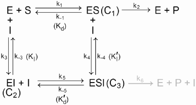
Schematic for a reaction involving an enzyme, substrate, and mixed inhibitor. The inhibitor binds both the free enzyme and the enzyme-substrate complex. The grayed reaction is for the case when the enzyme-substrate-inhibitor complex still has catalytic activity.
Substituting [Et] − [C1] − [C2] − [C3] for [E], as usual, gives a linear system of equations that is overdetermined unless we set ḰI = KI and Ḱd = Kd, in which case the system has rank 3 and we can find a unique solution for [C1], [C2], and [C3]. After more tedium, we get
with
And, of course
From this, we have that mixed inhibition reduces the maximum reaction rate to Vmax/α. Perhaps surprisingly, the half-maximal rate occurs when [S] = Kd.
We can generalize a little from this model to an inhibitor that modifies the reaction rate, rather than block the reaction entirely. Enzyme activity is frequently modified allosterically, most frequently by phosphorylation (addition of a phosphate group), and such modifications can either increase or decrease enzyme activity. Suppose that the EIS complex retains enzyme activity and dissociates with rate constant k6 to yield free product, inhibitor, and enzyme. The rate equations for [C3], [P], and [I] will be modified accordingly. The reaction rate becomes V = k2[C1] + k6[C3], and the solution for [C3] is:
and the reaction velocity is modified to:
12.5 Hemoglobin and the Hill equation
Many proteins bind multiple ligands, and it is often the case that the binding of one ligand modifies the kinetics of further binding. Hemoglobin, which carries oxygen in the blood, is the classical example of such behavior. Each hemoglobin molecule is made up of four subunits, each of which can bind one molecule of oxygen. Hemoglobin faces a challenge in that it must avidly bind oxygen diffusing from the air while circulating through the lungs, where oxygen concentration is high, but it must easily release to peripheral tissues, where oxygen concentration is low. Recall from Section 12.1.1 that, for a single ligand the fraction of ligand bound to a protein, θ is:
If this were the case, the oxygen saturation curve would be hyperbolic, and hemoglobin would be unable to both tightly bind oxygen in the lungs and deliver it to tissue [2] (see Figure 12.3). Instead, hemoglobin oxygen saturation changes sigmoidally. This is a consequence of cooperativity: when an oxygen molecule binds to a single subunit, the overall conformation of the molecule is changed so that it becomes much easier for oxygen to bind to the other subunits.

Hypothetical oxygen-hemoglobin dissociation curves. The two dotted curves are examples of no cooperativity: the top curve binds oxygen adequately in the lung, but does not release oxygen in the tissues, where it is needed. The lower curve releases oxygen to tissue, but binds it poorly in the lungs. The sigmoidal curve, which approximates actual dissociation curves, performs both tasks adequately, and is the solution to a Hill equation with Km = 27 and n = 3. Thus, cooperativity is essential to proper hemoglobin function.
The simplest and earliest model for cooperative binding was proposed by Hill in 1910 [8]. Hill was concerned with the binding of oxygen to aggregates of hemoglobin subunits in solution, and considered the case of an n subunit aggregate, Hbn, binding n oxygen molecules:
where Kd is the dissociation constant for Hb-O2 binding. Hill determined that an equation of the type
where x is O2 concentration, could explain observed oxygen-dissociation curves. He did not ascribe any mechanistic meaning to the equation, i.e. it is empirical. Following Nelson and Cox [2], the Hill equation can be taken to represent the scenario of perfect cooperation in ligand binding: either all ligands bind simultaneously and saturate the protein, or none do. To see this, consider n ligands, S, binding a protein:
Following reasoning similar to that in Section 12.1.1, we arrive at the Hill equation:
We can rewrite this as:
A plot of log(θ/(1− θ)) versus log[S] is called a Hill plot, and if cooperation is perfect, then the slope, nH, should equal n. In practice, cooperation is never perfect (nH < n), and nH, called the Hill coefficient, approximates the degree of cooperativity. If nH > 1, then there is positive cooperativity. If nH < 1, a rare occurrence, then cooperativity is negative, i.e. binding of one ligand inhibits bind by others.
12.6 Monod-Wyman-Changeux model
In 1965, Monod, Wyman, and Changeux [12] proposed a model (MWC model) for cooperative binding of ligands to protein, with hemoglobin principally in mind. We define an oligomer as a polymeric protein with several identical subunits, and define a single subunit as a protomer. Monod et al. based their model on the following assumptions:
- An allosteric protein is an oligomer, and all its promoters occupy equivalent positions, implying that there exists at least one axis of symmetry.
- There is exactly one ligand binding site on each protomer, and each site is identical.
- The oligomer has at least two conformational states, which it may reversibly transition between.
- When the protein goes from one state to the other, its molecular symmetry is conserved. That is, all protomers must always be identical.
Following Monod et al.’s original derivation and notation, we consider the case of a single ligand, F, binding an oligomer. We assume that oligomer has exactly two states, a “tight” state that has low ligand affinity, and a “relaxed” state that has high affinity for the ligand. As a consequence of the symmetry assumption, a change in protein conformation changes the ligand affinity of all binding sites. When free of all ligands, these two states are in equilibrium with equilibrium constant L. Let n represent the number of protomers and hence the number of homologous binding sites. A oligomer with i ligands bound is represented by Ri or Ti, whether it is in the tight or relaxed state. Let KR = krd/kra and KT = ktd/kta be the dissociation constants for ligand binding to a single stereospecific site. Importantly, the model does not allow transition between the Ri and Ti for i > 0. Therefore, cooperativity in this model refers to the ability of ligand binding to (temporarily) “lock” the protein into the relaxed (or tight) state. We have the reaction scheme:
It is important to note that the rate constants vary, reflecting the number of binding sites available and the number of ligands currently bound. We assume that the system is in equilibrium, yielding the equilibrium equations from mass action:
Finally, the fraction of protein in the R state is given by
and the fraction of actual ligand-binding sites bound is:
Using the equilibrium equations, we arrive at
where
Monod et al. determined graphically that cooperativity, as measured by the curvature of the lower part of a ȲF versus α curve, is most pronounced when c is small and L is large. If c is small, then and ligand binding in the relaxed state is much stronger. If L is large, then the free oligomer has a strong tendency to be in the tight state. Ligand binding “locks” the previously free protein into the relaxed state, subsequent ligand binding will occur far more readily, and cooperativity is therefore strong. Thus, these two observations make physical sense.
Note that if c = 1, i.e. ligand binding occurs at the same rate in the tight and relaxed states (KR = KT), then regardless of the value of L, ȲF reduces to the case where there is no cooperativity:
This also makes perfect physical sense.
References
[1] Keener J, Sneyd J: Mathematical physiology. New York: Springer Sci-ence+Business Media, 2004.
[2] Nelson DL, Cox MM: Lehninger Principles of Biochemistry (5th ed.). New York: W.H. Freeman, 2008.
[3] Quílez J: A historical approach to the development of chemical equilibrium through the evolution of the affinity concept. Chem Educ Res Pract 2004, 5:69–87.
[4] Lund EW: Guldberg and Waage and the law of mass action. J Chem Educ 1965, 42:548–550.
[5] Guldberg CM, Waage P: Avhandl. Norske Videnskaps-Akademi Oslo. Mat Natorv Kl 1864, 35.
[6] Guldberg CM, Waage P: Etudes sur les Affinites chimique. Ghent, Belgium: Brogger & Christie, 1867.
[7] Guldberg CM, Waage P: J Prakt Chem 1879, 19, 69.
[8] AV Hill: The possible effects of the aggregation of the molecules of haemoglobin on its dissociation curves. J Physiol. 1910, 40:iv–vii.
[9] Michaelis L, Menten ML: Kinetik der Invertinwirkung. Biochem Z 1913, 49:333-369.
[10] Briggs GE, Haldane JBS: A note on the kinetics of enzyme action. Biochem J 1925, 19:338-339.
[11] Sawday J: Engines of the Imagination: Renaissance Culture and the Rise of the Machine (p. 240). New York: Routledge, 2007.
[12] Monod J, Wyman J, Changeux JP: On the nature of allosteric transitions: A plausible model. J Mol Biol 1965, 12:88–118.
1A common textbook example of competitive inhibition is treatment of methanol poisoning. Methanol (“wood alcohol”) is metabolized to formaldehyde by the same enzyme (alcohol dehydrogenase) that metabolizes ethanol (“drinking alcohol”). Therefore, ethanol is used as a competitive inhibitor to slow the rate of formaldehyde formation while methanol is excreted by the kidneys.
2As Gottfried Wilhelm von Leibniz once remarked [11], “It is unworthy of excellent men to lose hours like slaves in the labour of calculation which could safely be relegated to anyone else if machines were used.”