
Chapter 9
Models of Chemotherapy
Modern chemotherapy and antibiotics arose in the same era, between the two world wars through World War II. The sulfonamides were introduced in 1935, and penicillin followed in 1940. The era immediately before and after World War II was revolutionary in the treatment of infectious disease.1 Rapidly fading was the therapeutic nihilism of the previous era, and many once deadly diseases were now easily curable. As Papac points out in her review of the beginnings of cancer chemotherapy [57], there was a (sadly doomed) hope that the “magic bullet” concept enjoying so much success in antimicrobial therapy would be applicable to cancers. Despite (and partly because of) their success, from the moment of their introduction, both antibiotic and anticancer agents have been plagued by the evolution of resistance. Understanding the evolution of resistance in cancer is a central goal of this chapter.
Cancers are resistant to systemic chemotherapy for at least three major reasons. First, as tumors advance, their growth fraction decreases. Therefore, since chemotherapy preferentially targets rapidly dividing cells, kinetic resistance to treatment tends to develop. Second, drug penetrance into the tumor microenvironment often declines due to high interstitial fluid pressure, drug wash-out, impaired blood flow and large inter-capillary distances within advanced tumors. Finally, and most importantly, heritable resistance to essentially any drug can be conferred by random genetic mutations followed by natural selection, which readily results in tumors (or microbial populations) refractory to treatment.
The “Norton-Simon” and “Goldie-Coldman” hypotheses have been influential in understanding kinetic and genetic resistance, respectively, and optimizing treatment regimens to minimize resistance. The Norton-Simon hypothesis, which describes tumor growth using the Gompertz model, has led to the notion of dose-density in chemotherapy scheduling. The Goldie-Coldman model considers the acquisition of drug resistance via random mutations in individual cells. We devote a significant portion of this chapter to these historically important models and several extensions and modifications of them. In addition, we look at antimicrobial chemotherapy, including the mutant selection window hypothesis and the role of synergy in selecting for resistance in multi-drug regimens.
In this chapter we also introduce pharmacokinetics and pharmacodynamics models, which describe distribution of drugs in the body and their physiologic effects. These highly mathematical fields have long been informed by dynamical models of the physiologic systems studied. Pharmacokinetic models, some more complex than others, are used to study the distribution into the body of essentially all drugs. Dose-response curves, which describe the relationship between drug dose, exposure time, and cytotoxicity to cancer cells, can be understood using simple dynamical models. More complex dynamical models have also been proposed to describe the uptake and intracellular action of antineoplastic agents. Several mathematical models specifying a given spatial geometry have been used to study the delivery of chemotherapy to tumors, the tumor spheroid and tumor cord being the two most common geometries used.
Our goals for this chapter are to (1) develop a basic mathematical basis for commonly observed dose-response curves for anticancer cancer agents, and to further study representative models of in vitro uptake and the intracellular dynamics, (2) develop the basic principles of pharmacokinetics and drug transport within the body and the spatial environment of the tumor, (3) optimize chemotherapy regimes to overcome kinetic resistance, (4) model the evolution of drug resistance in neoplastic cells.
9.1 Dose-response curves in chemotherapy
In Chapter 11 we largely focus on cellular response to radiation and how repair processes give rise to the observed dose-response curves. Here, in the context of chemotherapy, the situation is complicated by the dynamics of agent delivery and its intracellular processing, which we briefly discuss.
9.1.1 Simple models
The log-kill model for cancer cells was first established by Skipper and colleagues [62, 63] in the 1960s and early 1970s, who studied experimental tumors and found that the cell-kill of exponentially expanding tumor cell populations increased logarithmically with dose, giving the log-kill or log-linear model. That is, the surviving cell fraction, S, is given by
S=exp(−kD), (9.1)
where D is the total dose and k is a scaling parameter. An extension of this includes dependence upon drug concentration, C, and the time of drug exposure, T:
S=exp(−kC×T). (9.2)
The quantity C × T is the area under the curve (AUC) for the drug concentration vs. time curve. (Note that this notation is used even for non-constant drug concentrations.) For specific agents, survival relationships are generally determined by in vitro assays. There are a number of such assays, but the standard is the clonogenic assay. That is, an assay is performed where two cell populations of equal initial size are grown under conditions for exponential expansion. One population, NT , is exposed to the agent being tested, and the other, NC, serves as the untreated control. The surviving fraction S after time T is given as
S=NT(T)NC(T). (9.3)
This is taken as a surrogate for the expected cell kill, K = 1 − S. However, even for cell-cycle nonspecific drugs, cell kill is usually greater for actively proliferating than quiescent cells. The latter can make up a substantial portion of an in vivo tumor, and in vitro cytotoxicity does not directly predict in vivo toxicity, but the two are generally assumed to be correlated.
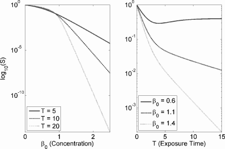
The log-linear model for the AUC can successfully predict in vitro cell survival and clinical response for a number of agents, and is generally considered to apply well to most cell cycle phase-non-specific (PNS) drugs. Several representative dose-response curves from Drewinko et al. [18] that can be described to some degree using the log-kill model are shown in Figure 9.1.
![Figure showing dose-response curves for three anticancer agents incubated in agent-containing medium for 1 hour. The data is from Drewinko et al. [18], and response curves for both exponential growth phase (proliferating) and plateau phase (non-proliferating) cells are shown. Note that proliferating cells are usually, but not always, more sensitive. The log-kill model applies directly for the first agent, doxorubicin. The curve for BCNU displays a “shoulder” region, where the surviving fraction is linear in AUC. This is generally interpreted as signifying recovery by some cells from sublethal damage, and the shown curve-fit is a superposition of a linear and exponential model. The curve for bleomycin is biphasic and is described by a double-exponential model.](http://imgdetail.ebookreading.net/math_science_engineering/24/9781498785532/9781498785532__introduction-to-mathematical__9781498785532__image__fig9-1.png)
Dose-response curves for three anticancer agents incubated in agent-containing medium for 1 hour. The data is from Drewinko et al. [18], and response curves for both exponential growth phase (proliferating) and plateau phase (non-proliferating) cells are shown. Note that proliferating cells are usually, but not always, more sensitive. The log-kill model applies directly for the first agent, doxorubicin. The curve for BCNU displays a “shoulder” region, where the surviving fraction is linear in AUC. This is generally interpreted as signifying recovery by some cells from sublethal damage, and the shown curve-fit is a superposition of a linear and exponential model. The curve for bleomycin is biphasic and is described by a double-exponential model.
Dose-response curves when the growth dynamics of the clonogenic assay are logistic (see Exercise 9.2). Constant parameter values are K = 10, α = 1, and N0 = 1. They are ad-hoc and for demonstrative purposes only.
For many cell cycle phase-specific (PS) drugs, cytotoxicity is not a simple function of AUC. Time of exposure may be more important than drug concentration, and plateaus in cytotoxicity are observed with increasing drug concentrations. One modification of the AUC model that accounts for differential importance of concentration and time is the pharmacodynamic model applied to chemotherapy by Adams [1]:
Cn×T=k, (9.4)
where n and k are empirically determined parameters. When n = 1, drug concentration and time are equally important and the model is equivalent to the AUC model. If n < 1, cell kill increases less with increasing dose than predicted by the AUC, and concentration is, in a sense, less important than exposure time. If n > 1, cell kill is greater than predicted by the AUC for a given concentration, and drug concentration or dose is more important than exposure time. Broadly speaking, this model can predict whether it is better to maximize drug concentration or exposure time for a given antineoplastic agent. Several other groups have also used a Hill function to model cell survival, e.g. [22, 23, 46].
9.1.2 Concentration, time, and cyotoxicity plateaus
While the simple log-linear model describes some data sets well, many dose-response curves have a two-phase appearance in which cytotoxicity plateaus with either dose or exposure time. Such curves are sometimes described as concave upward. Some authors have interpreted a concave upward curve as indicating the existence of a resistant sub-population of cells. There are several mechanisms that can explain a two-phase response (cytotoxicity plateau) for large drug doses for both cell cycle phase-specific (PS) and non-specific (PNS) drugs. In summary, saturation effects in either drug transport or saturation of the drug target can cause a plateau for either drug class. The instability of some PNS drugs in medium explains plateaus for these agents. Toxicity in PS drugs can be explained as a direct consequence of cell cycle specificity. We defer further discussion of cell-cycle specific chemotherapy to Section 9.6.
9.1.3 Shoulder region
The shoulder region seen in chemotherapy dose-response curves is similar to that seen in radiotherapy dose-response curves. Such a curve is predicted by models of DNA double-strand break interaction and repair in radiotherapy, and it has been generally assumed that a similar mechanism is at work in chemotherapy curves.
9.1.4 Pharmacodynamics for antimicrobials
We briefly mention dose-response pharmacodynamic models, which have been mostly applied to antimicrobial agents; the reader may consult Mueller et al. [52] for a more substantive treatment. A common measure of drug efficacy remains the minimum inhibitory concentration (MIC). The MIC is usually defined as the lowest concentration that completely inhibits visible bacterial growth in vitro after a 24-hour incubation period [52].
The efficacy of an in vivo course of therapy is often estimated using the serum concentration of the drug and the MIC as determined in vitro. The most commonly used metrics are the time above the MIC (T > MIC), the ratio of peak serum concentration to MIC (Cpeak / MIC), and the serum AUC over the MIC (AUC / MIC) [52]. Such approaches are problematic for many reasons; e.g., serum concentration does not necessarily reflect drug concentration at the infection site, and using the MIC alone falsely assumes an effect/no-effect phenomenon for microbes exposed to a drug.
The cytotoxic response saturates with drug concentration for many antimicrobials, leading to the fairly commonly used Emax model for drug effect. For exponentially growing bacteria, N(t), drug-induced death is modeled by a Hill function and we have the simple equation:
dNdt=N(k0−kmaxCtEC50+Ct), (9.5)
where Ct is the drug concentration at a given time, k0 is the unperturbed growth rate, kmax is the maximum killing rate, and EC50 is the drug concentration of half-maximal activity. Example Emax models may be found in [41, 71]. These models are also interesting because they combine non-trivial pharmacokinetics for the experimentally determined drug distribution within the body with a pharmacodynamic Emax model.
9.2 Models for in vitro drug uptake and cytotoxicity
Drug transport across the cell membrane generally occurs by three different mechanisms: (1) passive diffusion, (2) facilitated diffusion, (3) active carrier-mediated transport. At least some passive diffusion occurs for most small drugs, and it is the only means of transport for many anticancer agents. For passive diffusion, the flux across the membrane is proportional to the concentration difference across the membrane and the membrane surface area:
J=PA(SE−SI), (9.6)
where A is the surface area, SE is the extracellular concentration, SI is the intracellular concentration, and P is a permeability constant. Passive diffusion is also generally taken to imply that uptake and efflux are linearly related to extracellular and intracellular drug concentration, respectively. The ratio of drug concentration in the intracellular water to extracellular drug concentration never exceeds unity for drugs that are transported only by diffusion. Note that this does not imply that the overall intracellular:extracellular drug ratio never exceeds unity, as intracellular drug can bind extensively to cellular components.
Many drugs are incidentally similar to natural substances that are transported by membrane-bound carriers, and active transport is the dominant mechanism for trans-membrane transport for a number of anticancer agents.
Once inside the cell, the drug must exert its effect by interacting with intracellular elements, such as DNA. It also may be metabolized or actively excreted by the cell, and damage may be repaired by cellular mechanisms.
9.2.1 Models for cistplatin uptake and intracellular pharma-cokinetics
We briefly mention cisplatin as a model drug to study the mechanistic basis for dose-response curves. Cisplatin forms mono- and bifunctional DNA adducts that cross-link the cellular DNA, and the kinetics of such DNA interaction have been quantified. Binding to intracellular thiols detoxifies cisplatin, and DNA repair mechanisms can repair cisplatin:DNA lesions.
Sadowitz et al. [60] developed a simple model to describe cisplatin uptake and intracellular detoxification, and it considers the following behaviors: (1) uptake from the extracellular medium to the cytoplasm, (2) transfer of cisplatin from cytoplasm to the nucleus, (3) reaction of cistplatin with cytoplasmic thiols, (4) binding of cisplatin to the DNA to form DNA adducts, and (5) repair of platinum:DNA adducts.
The variables considered, all in units of concentration (µM), are cytoplasmic cisplatin, C(t), nuclear cisplatin, N(t), cytoplasmic thiol (sulfhydryl), S(t), free nuclear DNA, D(t), and cisplatin:DNA adducts, A(t).
Transport across the cell membrane is assumed to occur by simple diffusion, and transfer between the cytoplasmic and nuclear compartments is similarly assumed to be a diffusion process. The DNA and nuclear cisplatin interact according to second-order kinetics, as do cytoplasmic cisplatin and thiols. Thiols also enter the cell by simple diffusion, and DNA is repaired according to first-order kinetics. These considerations yield the full model:
dCdt=ka(Ce−C)−kbCS−kc(C−N), (9.7)
dNdt=kc(C−N)−kdND, (9.8)
dSdt=−kbCS+kf(Se−S), (9.9)
dDdt=−kdND+keA, (9.10)
dAdt=kdND−keA, (9.11)
where Ce and Se are the constant extracellular cisplatin and thiol concentrations, respectively, and all other parameter meanings are straightforward to interpret. Assuming that the free DNA concentration is nearly constant, the term kdN D for cisplatin-DNA interaction can be replaced by kdD0. We present this model as an example of applying basic chemical kinetic concepts to the topic and do not comment on it further. El-Kareh and Secomb [22] also proposed a simple model for cisplatin uptake and DNA binding by first-order kinetics.
9.2.2 Paclitaxel uptake and intracellular pharmacokinetics
We study a model of paclitaxel uptake and intracellular pharmacokinetics developed by Kuh and colleagues [44] that successfully described paclitaxel in vitro dynamics. Paclitaxel is a mitotic inhibitor that binds to tubulin and induces polymerization of microtubules. Paclitaxel inhibits microtubule dynamic remodeling, and at high doses it increases cellular microtubule mass. It is highly protein bound in the extracellular space, and within the cell it is almost entirely bound to cellular components. Overall, the model accounts for the following behaviors.
- Transport across the cell membrane of free drug by simple diffusion.
- Saturable binding of paclitaxel to extracellular proteins within the medium.
- Saturable and non-saturable binding of paclitaxel to cellular components.
- Time and concentration dependent changes in microtubule mass. Such microtubules serve as cellular paclitaxel binding sites, and this increase in microtubule mass increases cellular saturable binding.
- Time and drug concentration dependent changes in cell number.
The model derivation is somewhat non-standard and clever. The experiment considered 106 cells incubated in 1 ml of medium. Six drug populations are explicitly considered in the model derivation: the total amount of intracellular drug (AT,c), the total amount of drug in the medium (AT,c), the total concentration of intracellular drug (CT,c), the total concentration of drug in medium (CT,m), and the concentrations of free (versus bound) drug within the cell (CF,c) and medium (CF,m).
The total amounts of cellular and extracellular drug are simply
AT,c=Vc×CT,c, (9.12)
AT,m=Vm×CT,m, (9.13)
where Vc is the total cellular volume, and Vm is the volume of the medium. Differentiating and applying the product rule implies that
dAT,cdt=VcdCT,cdt+CT,cdVcdt, (9.14)
dAT,mdt=VmdCT,mdt+CT,mdVmdt. (9.15)
It is assumed that the volume of the medium stays constant, so the second term for extracellular drug can be neglected. The change in both drug amounts can also be expressed as a function of the concentration differences of free drug across the membrane. Therefore, altogether we have that changes in the total drug amounts can be expressed as follows:
dAT,cdt=VcdCT,cdt+CT,cdVcdt=CLfN(CT,m−CT,c), (9.16)
dAT,cdt=VmdCT,cdt=CLfN(CT,c−CT,m), (9.17)
where CLf is the clearance (i.e., diffusion) rate of free drug across the cell membrane per cell, and N is the total number of cells.
The total number of cells, and hence the total cellular volume, Vc, is not constant, as the cell population in this experimental setup either expands or contracts exponentially. At low paclitaxel concentrations there is a small growth rate overall, while at higher concentrations there is net death. Instead of making the change in N a function of cellular drug concentration, Khu et al. determined clonogenic expansion as an empirical function of drug concentration in the medium. That is,
N(t)=N(0)ekNt, (9.18)
where the parameter kN is determined empirically as a function of the initial drug concentration in the medium; i.e., kN = kN(Ctotal,m(0)). Also, total cellular volume can be expressed as
Vc=V0N=V0N(0)ekNt, (9.19)
where V0 is the volume of a single cell.
Next we consider drug binding to cellular components and proteins. Instead of explicitly modeling the time-dependent binding of intracellular drug to cellular components and extracellular drug to proteins, the authors use the steady-state expressions for total drug concentrations as a function of free drug. For saturable binding of a ligand to a protein, the concentration of bound protein:ligand can be expressed as a function of free ligand in general terms. Specifically,
BCK+C, (9.20)
where B is the number of binding sites, C is the concentration of free ligand, and K is a constant. This follows from standard chemical kinetics analysis. For non-saturable binding, Khu et al. assumed that the bound drug is a linear function of free drug. It follows that total drug concentrations can be expressed as
CT,c=CF,c+BcCF,cKd,c+CF,c+NSB×CF,c, (9.21)
CT,m=CF,m+BmCF,mKd,m+CF,m, (9.22)
where Bc(t) and Bm are the total number of intracellular and extracellular saturable binding sites, respectively. Note that Bc(t) is a function of time, and N S B is the proportionality constant for non-saturable binding sites within the cell; there is no non-saturable binding in medium.
These equations are quadratic in CF,c and CF,m. Some algebra yields the (positive) solutions for CF,c and CF,m in terms of CT,c, CT,m, and several parameters:
CF,c=−B+(B2+4(1+NSB)Kd,cCT,c)122(1+NSB), (9.23)
CF,m=−A+(A2+4Kd,mCT,m)122, (9.24)
A=Kd,m+Bm−CT,m, (9.25)
B=(1+NSB)Kd,c+Bc(t)−CT,c. (9.26)
We now discuss the time dependency of Bc(t). Paclitaxel binds saturably to tubulin and microtubules. However, such binding also increases the stability of microtubules and, at high drug concentrations, increases the mass of microtubules. Therefore, the number of intracellular binding sites available to paclitaxel increases with intracellular paclitaxel binding. This feedback loop was not directly modeled by Khu et al., but the time-dependent increase in microtubule mass was instead determined as an empirical function of the initial extracellular drug concentration:
Bc(t)=Bc0(1+kB,ct), (9.27)
kB,c=kB,c(CT,m(0)). (9.28)
The number of binding sites increases linearly in time with slope kB,c, which is determined empirically as a function of the initial drug concentration in the medium.
Finally, using equations (9.14) and (9.15), solving in terms of dCT,c/dt and dCT,m/dt and substituting the algebraically determined solutions for CF,c and CF,m yields a final system of 2 differential equations:
dCT,cdt=(CF,m−CF,c)CLfV0−kNCT,c, (9.29)
dCT,cdt=(CF,c−CF,m)CLfN0ekNtVm. (9.30)
9.3 Pharmacokinetics
Pharmacokinetics describes how drugs are distributed in and eliminated from the body. Three broad approaches have traditionally been used in this field. The first is compartmental modeling, where the body is divided into one or more discrete compartments (often aggregations of multiple tissue types) into which drug distributes. Typically, exchange occurs between the compartments according to first-order kinetics. Physiological modeling employs anatomical compartments (plasma, liver, kidney, etc.) and blood flow rates between the compartments govern drug distribution. Model-independent pharmacokinetics are used to characterize the distribution and elimination of drug in plasma without using any complex underlying model. Simple quantities such as plasma area under the curve (AUC), volume of distribution (VD), and elimination half-life (t1/2) are measured under this approach.
One-compartment model. It is necessary to introduce a few basic concepts, which we do so in the context of a one-compartment model with intravenous drug infusion. The dynamics of such a model are shown schematically in Figure 9.3. The first important concept is the (apparent) volume of distribution (VD), which is the volume that the drug in plasma is “effectively” diluted in. That is, the plasma concentration, C, is related to the amount of drug in the body, A, as follows:
C=AVD. (9.31)
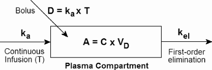
Schematic for one-compartment pharmacokinetic model with either continuous drug infusion at rate ka for time T, or a bolus of total dose D.
VD=AC. (9.32)
The volume of distribution gives an idea of how extensively a drug distributes from the plasma to body tissues. Typical volumes of body compartments are 3 L for the plasma (the non-cellular component of blood), 5 L for blood, 15 L for all extracellular water, and 42 L for total body water [68]. Therefore, if VD = 3 L, then the drug is sequestered entirely in the plasma; a VD of 5 L implies that it stays within the blood but freely enters erythrocytes. In general, the larger the VD the more extensively a drug distributes into body tissues. Many drugs also bind extensively to plasma proteins, principally albumin. Such bound drug is very slow to exit the plasma, and only free drug should be considered in VD calculations.
The first order plasma elimination rate, kel, is (obviously) the rate at which drug is eliminated from plasma. It is important to note that this rate depends upon the distribution of drug between plasma and tissues, and thus depends upon the volume of distribution.
The plasma clearance Clp, unlike kel, is independent of VD. Plasma clearance rate has units of volume per time (e.g. L/hr), and reflects the volume of plasma from which drug is completely removed in a unit of time. Thus, it simultaneously measures both the rate at which the clearing organ excretes the substance and the rate of plasma flow through the organ [64], which is typically the kidney. Assume the kidneys are responsible for the clearance. Plasma flow through the kidneys is constant and a certain volume of this plasma will be cleared per unit time; this is precisely the clearance parameter Clp. If the volume of distribution is large, the plasma drug concentration will be small. Only a small amount of drug will be cleared per unit time and therefore kel will be small. Mathematically, we have the following relationships:
dAdt=ClpC=−kelA=−kelVDC, (9.33)
Clp=kelVD. (9.34)
The plasma area under the curve (AUC) is simply the integral of drug concentration C(t) over time:
AUC=∫∞0C(t)dt. (9.35)
The AUC has units concentration × time (e.g., mg hr L−1). Interestingly, dose, plasma clearance, and plasma AUC are all related. For bolus of size D, the initial drug concentration is C0 = D/VD, and C(t) = C0 exp(−kelt). Integrating gives:
AUC=∫∞0DVDe−keltdt=DVDkel=DClp. (9.36)
This relationship also holds for any infusion schedule as long as the total dose delivered is D.
Finally, using these concepts we can easily frame the dynamics of the one-compartment model with an initial bolus of size D in the following way:
dAdt=−kelA=−kelVDC=−ClpC=−ClpAVD=−DAUCC, (9.37)
dCdt=1VDdAdt, (9.38)
A(0)=D, (9.39)
C(0)=DVD. (9.40)
For a continuous infusion at rate ka from time 0 to T the equations are similar, but with a “+kaH(T − t)” term on the right side.
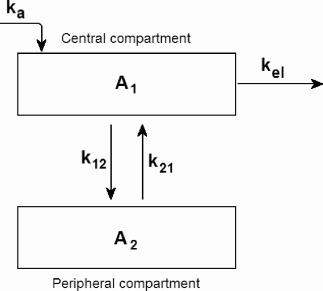
Two-compartment model. We now present the two-compartmental pharmacokinetic model, which explicitly models the distribution of drug from the central compartment (plasma) to the peripheral compartment (tissue) (Figure 9.4). The time course of plasma drug concentration for a two-compartment model is markedly different from the one-compartment model. It is characerized by two phases: the initial distribution (α) phase where plasma drug concentration rapidly drops as it is sequestered in tissue, and a much slower elimination (β) phase where plasma and tissue drug are essentially at equilibrium and drug clearance (i.e., kel) is slower. This pattern is shown in Figure 9.5.
![Figure showing two-phase plasma drug concentration dynamics for a two-compartment model. Shown is the two-compartment model for doxorubicin plasma concentration from Greene et al. [31] with A = 4425 nM, α = 4.159 hr−1, B = 87 nM, and β = 0.02530 hr−1.](http://imgdetail.ebookreading.net/math_science_engineering/24/9781498785532/9781498785532__introduction-to-mathematical__9781498785532__image__fig9-5.png)
Two-phase plasma drug concentration dynamics for a two-compartment model. Shown is the two-compartment model for doxorubicin plasma concentration from Greene et al. [31] with A = 4425 nM, α = 4.159 hr−1, B = 87 nM, and β = 0.02530 hr−1.
Using the so-called microscopic rate constants, the differential equations describing the amount of drug in the two compartments are the following:
dA1dt=k21A2−k12A1−kelA1, (9.41)
dA2dt=k12A1−k21A2, (9.42)
where A1 is the amount of drug in the central compartment (plasma) and A2 is the amount in the peripheral compartment (tissue). Typically, the drug concentration in the central compartment (plasma) is of interest and can be easily measured.
For a bolus infusion, the plasma concentration, C, is usually reported using the following model:
C(t)=Ae−αt+Be−βt. (9.43)
This model is popular because of its simplicity and because the so-called macroscopic rate constants A, α, B, β can be estimated graphically from a plot of plasma concentration vs. time. In general A » B and α » β. Heuristically, this model can be thought of as the superposition of two separate models. Because A » B, in early time A exp(−αt) » B exp(−βt), and during this time the drug is distributing from the plasma to peripheral tissues, and C(t) = A exp(−αt) is the model for the distribution phase. The concentration in this model quickly goes to zero, as α is large. Following distribution, C(t) = B exp(−βt) is the model for plasma concentration during the elimination phase. Explicit expressions relating the macroscopic and microscopic rate constants can be derived (see [68] for details).
Extensions. The two-compartment model above can be extended to consider an arbitrary number of compartments, which may have various physical interpretations. The usual notation for a three-compartment model is:
C(t)=Ae−αt+Be−βt+Ce−γt. (9.44)
Another useful extension is to consider infusing a total dose D over the time interval (0, T), considering the two-compartment model as the explicit summation of two independent compartments:
dC1dt=ATH(T−t)−αC1, (9.45)
dC2(t)dt=BTH(T−t)−βC2, (9.46)
C(t)=C1(t)+C2(t). (9.47)
An analytic solution for C(t) can be found by integration. (We leave this as an exercise.)
9.4 The Norton-Simon hypothesis and the Gompertz model
Having covered some basics, we devote the next block of this chapter to models focusing on the optimal scheduling of treatment regimes. The influential Norton-Simon and Goldie-Coldman models are our major focus.
We begin our discussion of modeling in vivo cancer treatment with a coupling of the log-kill model and the Gompertz model for in vivo tumor growth. The Gompertz model is a sigmoidal growth curve often used to describe tissue growth. While derived from an actuarial model unrelated to biology, it can be interpreted as a model for growth that is initially exponential, but the rate of growth decreases exponentially with either time or organ size. There are multiple mathematical forms of the model, and the reader can consult Chapter 2 for a detailed discussion of growth curves in cancer. This simple growth law has been applied to human tumors and has motivated “dose-dense” treatment schedules for breast cancer chemotherapy.
9.4.1 Gompertzian model for human breast cancer growth
In 1988, Norton fit a Gompertzian model to human breast cancer growth [53], which we use as our tumor growth model for the remainder of this section. Recall from Chapter 2 that the model can take the following form:
dNdt=bNln(N∞N), (9.48)
which has solution,
N(t)=N0exp(k(1−exp(−bt))), (9.49)
where
k=ln(N∞N0).
Using this model, Norton estimated that breast cancer was typically diagnosed at a volume of about 5 mL of packed cells, corresponding to N0 = 4.8 × 10⁹ cells. Death occurred at a total cancer burden of 1 L, giving the lethal load NL = 1012 cells. Furthermore, N∞ = 3.1 × 10¹² cells (3.1 liters), and b had a log-normal distribution with mean −2.9 and standard deviation 0.71.
9.4.2 The Norton-Simon hypothesis and dose-density
Chemotherapy primarily targets rapidly dividing cells, and when multiple treatments are delivered, there is tumor regrowth between them. Under the Gompertzian model, the tumor growth rate attenuates with tumor age and size, implying that smaller tumors are relatively more susceptible to chemotherapy. Using this as theoretical motivation, Norton and Simon proposed the “Norton-Simon hypothesis”:
Therapy results in a rate of regression in tumor volume that is proportional to the rate of growth that would be expected for an unperturbed tumor of that size.
It follows from the Gompertz model (or any model of sigmoidal growth) that more closely spaced treatments will result in greater cell kill, as less regrowth will occur between treatments. Moreover, the tumor at the start of each treatment will be smaller, implying that the growth rate will be greater than for a larger tumor, and per the Norton-Simon hypothesis therapy will result in greater rates of regression.
9.4.3 Formal Norton-Simon model
In Norton and Simon’s original 1977 work [54], they proposed that cell kill due to some chemotherapy occurs at a rate proportional to the tumor growth fraction, giving the general tumor growth law under therapy:
dNdtGF(N)N(t)−L(t)GF(N)N(t), (9.50)
where GF(N) is the tumor growth fraction and L(t) is the current “level” of chemotherapy. Applying this concept to the Gompertz model, we have:
dNdt=bln(N∞N(t))︸growth fraction(N(t)−L(t)N(t)). (9.51)
Note that if L(t) = L0 is constant over time, then the analytic solution is simply
N(t)=N0exp((N∞N0)(1−e−b(1−L0)t))). (9.52)
Using this simple theoretical model, we can make several predictions concerning optimal scheduling of a total dose of chemotherapy, DT , delivered in K treatments. Norton and Simon’s primary result was that dose-density should be maximized. That is, the time interval between doses should be minimized. Dose-density is a somewhat nebulous concept, as there is no precise way to compare the “density” of two different regimes. Note that dose-dense is not equivalent to high-dose, as high doses widely spaced may not be very “dense” in time. Dose-density is also not equivalent to dose-intensity, which is the dose delivered per unit time. We can say that for a fixed total dose, a more intense schedule is also more dense.
The efficacy of a treatment regime is typically measured using two primary metrics:
- Cancer cell nadir: The lowest cancer cell count achieved. If the predicted nadir is very low, perhaps less than several hundred cells, then chemotherapy may be curative. That is, there is a reasonable probability that all cancer cells are eliminated and the cancer is totally cured. If there is a reasonable chance of cure, then the goal of chemotherapy is to minimize the nadir.
- Survival time: The total amount of time that the patient survives when chemotherapy is not curative. If there is not a reasonable chance of chemotherapy being curative (the tumor burden is too high, the tumor is metastatic, or poorly responsive to therapy, etc.) then the goal of chemotherapy is to maximize survival time.
We examine the Norton-Simon hypothesis applied to the Norton model for Gompertzian breast cancer growth computationally, using N0 = 4.8 × 10⁹ and assuming that death occurs at the lethal load NL = 1012 cells. For each treatment, we impose a constant level of drug, L(t), over some relatively brief interval—e.g., 24 hours. Our results may be summarized as follows:
- For a given dose DT divided into K treatments, the earlier that treatment is initiated the lower the cancer cell nadir. However, survival time is not affected by the time of treatment initiation.
- Spacing treatments more closely—i.e., using a more dose-dense treatment schedule—results in a lower cell nadir, but inter-treatment time does not affect survival time (see Figure 9.6).
- The number of treatments, K, into which a constant total dose is divided does not affect survival time, except if K is so large that tumor growth is markedly positive. Cell nadir increases monotonically with K.
- Increasing dose-density is relatively more beneficial, in terms of cell nadir, for more rapidly growing tumors.
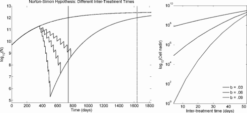
The left figure shows 10 treatments spaced either 15, 30, or 45 days apart under Gompertzian growth and the Norton-Simon hypothesis. The former, more dose-dense regime results in a lower cancer cell nadir, but all regimes converge to the same asymptotic growth curve and overall survival time is equivalent. The upper dashed line is the unperturbed growth curve, and patient death is expected to occur at the solid line for unperturbed growth and at the dotted line when treatment is applied. The right figure plots the cancer cell nadir vs. inter-treatment time (for 10 treatments) for tumors with different growth rate parameters (b), demonstrating that the benefit to dose density is greater for faster growing tumors.
Overall, the Norton-Simon model predicts that survival time, in the absence of a cure, is remarkably independent of the treatment schedule: the time at which therapy is initiated, the number of treatments, and the inter-treatment time are all unimportant. However, if the goal of therapy is to cure the tumor by eradicating all cancer cells—i.e., minimize the cancer cell nadir— then treatment should be initiated as soon as possible, inter-treatment time should be minimized (dose-density), and the total dose should be delivered in as few infusions as possible.
Since decreasing the cancer cell nadir transiently reduces the tumor burden without affecting overall survival time, dose-dense regimes may improve early survival and perhaps increase median survival time without affecting the longterm survival rate.
9.4.4 Intensification and maintenance regimens
Norton and Simon [54] argued that their model supports a treatment plan of initially moderately intense treatment to decrease tumor size and hence increase growth rate, followed by late intensification to take advantage of the increased growth fraction of a smaller tumor. Moreover, they argued that low-dose maintenance therapy likely has little effect on survival. From simulations, however, we can see that if the same total dose is delivered, it is irrelevant whether treatment employs a constant dose or early or late intensification. Under any model where cell-kill is proportional to drug concentration, if intensification involves an increase in total dose then it will be beneficial, but this is no profound result.
9.4.5 Clinical implications and results
In practice, drug sensitivity in tumors is heterogeneous, so combination chemotherapy with several agents is used, with agents given either sequentially, concurrently, alternating, or in some combination. The Norton-Simon model is interpreted to predict that dose-dense schedules with agents given in sequence, rather than concurrently or in alternating schedules, are best. The strategy is to eliminate all cells sensitive to each agent independently, which is best accomplished by a dose-dense schedule. Sequential delivery is therefore preferred because the dose level and density can be maximized when toxicity from concurrently delivered agents is absent.
When tested in clinical trials, dose-dense strategies have enjoyed modest success. The major trial supporting dose-density is the Cancer and Leukemia Group B Trial 9741 (CALGB 9741) [14], in which patients were treated with combination therapy by doxorubicin (A), paclitaxel (T), and cyclophos-phamide (C), in one of four sequences: (1) A-T-C with doses every 3 weeks, (2) A-T-C with doses every 2 weeks, (3) AC-T (i.e., A and C concurrent) every 3 weeks, or (4) AC-T every 2 weeks.
Dose-density was associated with improved disease-free and overall survival, and sequential and concurrent schedules were equally effective. This trial is important as it was purely a test of dose-density, while the interpretation of most trials purporting to test dose-density is complicated due to variations in treatment arms (e.g. total dose, number of cycles, etc. See [12] for a recent meta-analysis and review of such studies).
As an aside, we point out that any model with tumor regrowth between treatments, even simple exponential growth, would predict that a more dose-dense regime would result in a lower cancer cell nadir. Therefore, we cannot reasonably infer from modest clinical results that the Gompertz model is an accurate description of the natural history of individual breast cancers. See Chapter 7 for a discussion of associated controversies concerning the natural history of breast cancer.
9.4.6 Depletion of the growth fraction
We can see from its basic mathematical expression that the Norton-Simon model assumes that tumor growth fraction following treatment is equivalent to that of an unperturbed tumor allowed to grow to the same size:
dNdt=GF(N)N(t)−L(t)GF(N)N(t). (9.53)
The growth fraction is a function only of the current tumor size; i.e., GF = GF(N). This directly implies the basic tenant of the Norton-Simon hypothesis:
The efficacy of chemotherapy is proportional to the rate of growth of an unperturbed tumor of equivalent size.
Unfortunately, this ignores the perturbation in the underlying population age-structure caused by treatment. Proliferating cells are exclusively targeted under the Norton-Simon hypothesis, so there must be a dramatic reduction in proliferating cells following treatment. The growth fraction (at least immediately) following treatment is most likely reduced, not increased. Therefore, we have GF ≠ GF(N), and the growth fraction is a function of the number of actively proliferating cells, which is not a simple function of N (at least when the tumor cell population is not at a steady state distribution, which it most definitely will not be following cytotoxic treatment).
Gyllenberg and Webb showed that a system in which cells transition between quiescent (Q) and proliferating (P) compartments can exhibit Gom-pertzian growth kinetics [33]. (See Chapters 2 and 4 for details.) Kozusko, Bajzer, and colleagues [42, 43] later studied treatment under this model, and concluded that following treatment the tumor “is not the same tumor” and the Gompertz growth equation cannot be directly reapplied to determine the growth trajectory. Nor can it, then, necessarily be used to predict response to treatment.
In [43], analytic solutions for tumor growth following treatment are derived which demonstrate that treatment fundamentally alters the growth trajectory by changing the asymptotic tumor size, Nom, and if N/P is sufficiently small, tumor growth will be negative following the end of treatment. The authors also concluded, like Norton and Simon, that a dose-dense schedule is preferable and faster growing tumors respond better to dose density. However, they compared increasing, constant, and decreasing dose schemes and found that a decreasing schedule is best, contradicting Norton and Simon, who suggested dose intensification as a treatment strategy. Thus, a model giving gross Gom-pertzian kinetics but with an underlying population structure can differ in its predictions for optimizing therapy.
9.5 Modeling the development of drug resistance
While kinetic resistance plays a role in cancer treatment failure, evolution of intrinsically resistant cells is the major cause of treatment failure and ultimately death in cancer. This situation is somewhat analogous to the evolution of widespread antibacterial resistance among bacteria populations, which represents a growing threat to public health. Therefore, in this section we extend our discussion to models for antibacterial resistance as well. We begin with the enormously important work of Luria and Delbrück and later extensions by Lea and Coulson [45] which established the cause of resistance to viral attack in bacteria.
9.5.1 Luria-Delbrück fluctuation analysis
In their landmark 1943 paper [47], Luria and Delbrück attempted to determine the cause of bacterial resistance to bacteriophage infection. When bacterial cultures are challenged with a phage virus, the vast majority of bacteria are killed. However, the cultures tend to regrow, and when they do they resist infection by the same phage. Prior to Luria and Delbrück’s paper, two hypotheses had been suggested to explain this phenomenon. The first supposed that mutations conferring resistance arise prior to infection. When exposed to the phage, clones carrying these resistance mutations survive and repopulate the culture, passing their resistance to their offspring. In other words, resistance evolves by natural selection, although, oddly, Luria and Delbrück and most researchers following in their footsteps resist expressing the hypothesis in explicit Darwinian terms. The second hypothesis posits that bacteria develop a sort of immunity to the phage, analogous to mammalian immune memory. Under this hypothesis, the initial bacterial die-off is not complete; some bacteria, for whatever reason, heritable or otherwise, resist being killed. Those that survive then acquire some mechanism that blocks bacterial infection, and this acquired mechanism is somehow passed to their offspring. So, in summary, hypothesis one claims that resistance to the phage evolves, whereas hypothesis two supposed resistance is acquired.
Luria and Delbrück’s experimental test of these hypotheses has led to an experimental design called fluctuation analysis. Here is the approach:
Step 1. From a large parental culture of bacteria, take a number of samples and plate them on phage-impregnated media, so that only resistant variants will grow. If resistance is acquired, then some fraction of cells will acquire resistance and, assuming the probability of becoming resistant is small, the number of resistant variants will be approximately Poisson distributed (the actual distribution is binomial). That is, the variance equals the mean. If resistance is due to spontaneously arising, pre-existing mutants, the number of resistant variants recovered simply reflects the prevalence of mutants in the parental population and will also be Poisson distributed.
Step 2. Now, take a number of small samples from the parental culture (so that the likelihood of pre-existing mutants is vanishingly small) and expand these cultures in parallel to a fixed size. Then re-plate on selective media to determine the number of resistant variants. Under the acquired resistance hypothesis, resistance is not induced until the final challenge, and the total number of resistant variants should again be Poisson distributed. However, if resistance is due to selection for resistance mutations, the number of resistant cells will vary (“fluctuate”) widely as a consequence of rare mutations occurring at different points in time. In this case, variance will be much greater than the mean (rare early mutations imply a large mutant population). Analysis of these fluctuations provides a means to estimate mutation rates.
In the following sections we largely follow Luria and Delbrück’s original argument. Although it is a bit old-fashioned and not up to modern standards of rigor, we stick with it to help those interested in reading the original paper interpret the result. In outline, Luria and Delbrück first generate equations for the expected number of mutation events and the expected (or average) number of resistant cells (with some hand-waving). Then, they calculate the variance for resistant cells under the two competing hypotheses. Experimental results confirmed the predictions associated with the mutation-selection hypothesis, indicating that resistance arises by selection on pre-existing mutants rather than an acquired resistance. This process is summarized schematically in Figure 9.7.
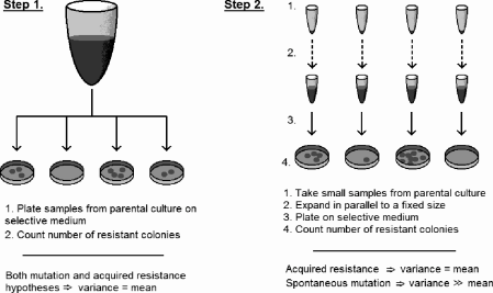
Schematic for Luria-Delbrück fluctuation analysis to distinguish between hypotheses for resistance to viral attack in bacteria.
9.5.1.1 Step 1: Expected number of mutations and resistant cells
Luria and Delbrück start with the assumption that laboratory bacterial populations grow exponentially. They normalized time such that a unit of time equals the average bacterial division time divided by ln 2. Therefore,
dNdt=N⇒N(t)=N0et, (9.54)
where N(t) is the bacterial population size at time t. (They use the notation Nt for N(t).) They also assumed that resistance mutations occur with a fixed probability with each cell division. They argue that, given their choice of time units, the probability that a single bacterium acquires a resistance mutation in a small time interval dt is α dt, and number of mutations, dm, which occur in this interval is given by
dm=αN(t)dt. (9.55)
To get the average number of mutations that occur in t ∈ (0, T), they integrate the following:
m=∫T0dm=∫T0αN(t)dt=∫T0αN0etdt=α(N(T)−N0). (9.56)
Assuming that the rate of mutations is small, Luria and Delbrück argue that the number of mutation events is Poisson-distributed. Therefore, the probability a culture of bacteria experiences no mutational events, P0, would be
P0=e−m. (9.57)
This is all well and good, but we are really interested in the number of resistant cells, not just the number of resistance mutations, that have arisen. Since mutations are passed vertically from mother to daughter cells, the number of mutant cells expands exponentially from all original mutant “foundresses.” So, let ρ(t) be the number of resistant cells in a bacterial population. Assuming these cells proliferate with the same kinetics as drug-senesitive cells,
dρdt=ρ+αN(t). (9.58)
Luria and Delbrück then integrate over the interval (0, T) assuming that no resistant cells are initially present (ρ(0) = 0) to obtain the expected (average) number of resistant cells:
ρ=αTN(T). (9.59)
From here, Luria and Delbrück argue that most experimental bacterial populations will not conform to this average. Because mutations in early generations are highly unlikely due to the small population size, in real experiments one typically sees ρ « αT N(T). Occasionally, however, early mutations will generate a very large resistant population, so it can happen that ρ » αT N(T). Nevertheless, for experiments of limited size, the observed average will typically be lower than that predicted by equation (9.59), making the average less useful in actual experiments. So, Luria and Delbrück derive an expression for the “likely average ρ” one can expect to see in real experiments, which they denote r. To find r, they solve equation (9.58) over the interval (T0, T) to obtain
r=αT(T−T0)N(T), (9.60)
where T0 is set to be the average time by which only a single mutation occurred in a group of C cultures. (So, T0 is a function of C.) From this and equation (9.56) they find that
1=αC(N(T0)−N0). (9.61)
Assuming N0 = 0 and noting that N(T0) = N(T) exp(T0 − T), substitution and some rearrangement of equation (9.61) yields
T−T0=ln[αCN(T)]. (9.62)
Substituting this into equation (9.60) yields a transcendental equation for r,
r=αN(T)ln[αCN(T)]. (9.63)
From here, two methods have been developed to estimate the mutation rate, α. The first, called the method of means, is to solve the transcendental equation (9.63) numerically for α. The second, or P0 method, uses P0, the fraction of cultures without resistance present. As above,
P0=e−m=e−α(N(T)−N0)≈e−αN(T)⇒α=−mN(T)−lnP0N(T). (9.64)
We have now generated predictions assuming the mutation hypothesis is true. The second step of Luria-Delbrück fluctuation analysis is to analyze the fluctuations to test these predictions.
9.5.1.2 Step 2: Test the mutation-selection hypothesis
To test hypothesis, Luria and Delbrück produce an estimate of the variance in number of resistant cells. They begin by estimating the partial distributions of number of resistant bacteria due to mutations arising in the time interval (T − τ, T − τ + dτ). We estimate that, in this interval,
dm=αN(τ)dτ=αN(T)e−τdτ. (9.65)
At the time of observation, T, they argue that each mutant clone arising in dτ has grown to size eτ. Therefore, the distribution of number of mutants from dτ has a mean eτ times greater and a variance e2τ times greater than the mean of the distribution of number of mutation events. Since this latter distribution is assumed to be Poisson, one has that
dρ=μN(T)dτ, (9.66)
vardρ=αN(T)dτ, (9.67)
Integrating over either (0, T) or (T0, T) gives:
varρ=αN(T)(eT−1), (9.68)
varr=αN(T)(eT−T0−1). (9.69)
Substituting T − T0 from equation (9.62) yields
varr=Cα2N(T)2. (9.70)
Finally, the ratio of variance to mean becomes
varrr=αCN(T)lnαCN(T). (9.71)
It follows that varr » r if αC NT » 1. This latter quantity represents the total number of mutants, so the variance will be very high as long as we expect a significant number of mutants to arise. In experiments, it is indeed observed that variance » mean, confirming the mutation-selection hypothesis.
9.5.1.3 Later work
In 1949, Lea and Coulson [45] derived a probability generating function for the distribution of mutants and proposed several new methods to estimate the number of mutants, and hence rate of mutation. For a review of theoretical work that followed over the next half century, see Zheng [70]. Foster [24] gives a fairly concise review of practical methods for estimating mutation rates.
9.5.2 The Goldie-Coldman model
Work following that of Luria and Delbrück confirmed and amplified their results so that by the time Goldie and Coldman published their original 1979 paper [28], it had become well established that microbial populations develop drug resistance through spontaneous, inheritable mutations that arise independently of the agent, and that the emergence of resistant phenotypes is the primary cause of antibiotic treatment failure. Assuming a similar process occurs during cancer treatment, Goldie and Coldman derived a simple, testable model for cancer chemotherapy resistance. The model assumes that all cancer cells have unlimited replicative potential, considers treatment with only a single drug, and assumes that cells are either sensitive or totally resistant to the drug. Let N represent the tumor size (say, mass of cells), µ be the mass of resistant cells, and let α and β be the rates per cell division at which cells mutate in and out of the resistant class, respectively. Furthermore, normal and mutant cells are assumed to follow the same growth kinetics. From these assumptions, Goldie and Coldman argued that the change in µ with a small change in N (ΔN) can be expressed as follows:
μ(N+ΔN)=μ+μNΔN︸growth of mutants+α(1−μN)ΔN︸mutation in−βμN︸mutation out. (9.72)
Expanding µ(N + ΔN) using Taylor’s theorem yields
μ(N+ΔN)=μ+dμdNΔN+O(ΔN2). (9.73)
Equating the two expressions, dividing by ΔN, and letting ΔN → 0 gives
dμdN=μN+α(1−μN)−βμN. (9.74)
If one assumes that resistance is a permanent condition (β = 0), then we have the following solution for µ under initial conditions N(0) = 1 and µ(0) = 0:
μ(t)=(1−N(t)−α)N(t). (9.75)
From this it easily follows that the fraction of resistant cells within the tumor at any time, F, is given by:
F(t)=μN=1−N−α, (9.76)
where time dependencies on the r.h.s. have been suppressed for brevity.
Alternatively, as mentioned in Chapter 7, one can derive the model from a differential equation giving the rate of change of µ with respect to time from first principles:
dμdt=(μN)dNdt︸growth of mutants+αdNdt(1−μN)︸muttion in−βdNdt(μN)︸mutation out. (9.77)
Note that model (9.77) is not particular to chemotherapy resistance; it represents a general model for the emergence of any mutant from a wild-type population.
An attractive property of this model is that the number of mutants does not depend upon any underlying growth law for the primary tumor: the instantaneous tumor size at any time gives the expected number of mutants. However, we can see that this is a consequence of the assumption that the cell division rate is precisely equal to dN/dt, which is not necessarily the case. For example, rapid proliferation nearly balanced by rapid cell death gives a very small dN/dt, but mutants will emerge far faster than predicted by the model. An alternative model can be derived that accounts for this behavior, and we suggest it as a student project.
Now let us return to the model and its predictions. As pointed out in the original paper, rare mutations early in time lead to a large mutant population later in time. Such mutations have a disproportional effect upon the mean number of mutant for a given tumor size, and therefore the number of mutant has a highly right-skewed distribution, and the expected value, µ, gives limited information. Goldie and Coldman confirmed this using a stochastic simulation of the model.
Now assume that the presence of any resistant mutants leads to treatment failure. To determine the probability that a tumor can be cured, we must determine the probability that a resistant colony has arisen at the time of diagnosis—i.e., the probability that at least one mutation has occurred. Because of its right-skewed distribution, the mean number of mutant cells µ is not a surrogate for the expected number of mutation events. Using arguments similar to those above, we can derive an expression for the probability that no resistant colonies exist in a tumor of size N, which we designate as ˆP
ˆP(N+ΔN)=ˆP(N)+dˆPdNΔN+O(ΔN2). (9.78)
For the small population increment ΔN, the rate at which mutants arise is approximately equal to the constant value αΔN. Therefore, the (random) number of mutations is approximately Poisson-distributed, and the probability that no mutation occurs during the interval ΔN is approximately
ˆP(ΔN)=exp(−αΔN). (9.79)
Finally, we have the following relationships:
ˆP(N+ΔN)=ˆP(N)׈P(ΔN)=ˆP(N)exp(−αΔN)=ˆP(N)(1−αΔN+O(ΔN2)). (9.80)
The last step uses the Taylor-series expansion for exp(−αΔN). Equating the right-hand sides of (9.78) and (9.80), dividing by ΔN and neglecting terms of O(ΔN2) gives the following:
dˆPdN=−αˆP(N). (9.81)
Integrating and applying initial conditions ˆP
ˆP=exp(−αN+α). (9.82)
So, the probability that no cell in the population acquires a mutation decreases exponentially with the total tumor size at a rate equal to α, the mutation rate per cell cycle. This and the expected number of mutant cells, µ, as a function of the logarithm of tumor size, ln N, are shown in Figure 9.8. From the figure it is apparent that the model predicts that with increasing tumor size there is a rapid transition from nearly curable to nearly incurable. This can also be seen with a few simple calculations. Suppose ˆP
ln(N05N95)=4.067=eln(2)×5.87. (9.83)
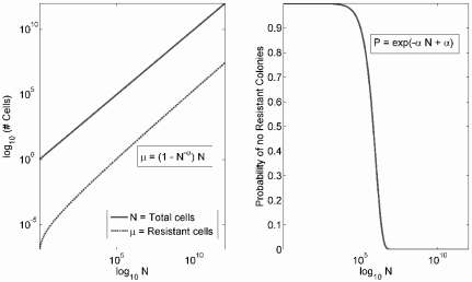
The expected number of mutant cells, µ, and the probability that no mutant colony exists, ˆP
The last point shows that under an exponential tumor growth model it takes just under six doubling times for a tumor to become nearly incurable. Therefore, the model predicts that treatment should be initiated as soon as possible, lest the window of opportunity be missed.
A reasonable range for α is between 10−5 and 10−8. Since about 109 cells must be present for cancer diagnosis, the probability that no treatment-resistant mutant exists by the time of diagnosis is essentially negligible. Even under very optimistic parameter values—e.g., α = 10−8 and N = 108—the probability of cure with a single agent is small. Therefore, the basic Goldie-Coldman model makes the following broad predictions:
- Treatment-resistant mutants arise early in a tumor’s natural history and are likely present at the time of clinical diagnosis.
- The tumor fraction that is resistant increases with tumor size.
- Treatment must be initiated as early as possible, as tumors rapidly transition from curable by a single agent to nearly incurable.
9.5.3 Extensions of Goldie-Coldman and alternating therapy
9.5.3.1 Two-drug Goldie-Coldman model
Several years after they published their original model, Goldie and Coldman extended their basic model to consider resistance to two non-cross-resistant drugs [30]. From this model, they concluded that non-cross-resistant drugs should be alternated as quickly as possible to minimize the probability that multi-drug resistant mutants arise during treatment. In the literature, this is generally regarded the major prediction of the Goldie-Coldman hypothesis.
The model considers two drugs, T1 and T2, and three populations of resistant cells. We represent singly-resistant mutants by R1 and R2, which are resistant to T1 and T2, respectively. Doubly resistant mutants are represented by R12. Cells mutate to become resistant to T1 and T2 at rates α1 and α2 per cell division; these rates are the same whether mutating from sensitive to singly resistant or from singly to doubly resistant classes. It is assumed that resistance to both agents must be acquired in a step-wise manner. Furthermore, the tumor is assumed to grow exponentially. These assumptions give a basic model similar to the one above:
dR1dN=α1(1−R1+R2N)−α1R1N+R1N, (9.84)
dR2dN=α2(1−R1+R2N)−α2R2N+R2N, (9.85)
dR12dN=(α1+α2)R1+R2N+R1+R2N. (9.86)
This model can also be rewritten using differential equations with respect to time, which we leave as an exercise. As above, the mean number of resistant cells does not tell the whole story, as rare mutants that arise early in time expand the mutant population greatly. The distribution of mutants is rightskewed, and we must determine the probability that no doubly resistant colony has arisen at the time of diagnosis or following treatment. To this end, first assume that when there are N0 sensitive cells, the number of cells resistant to Ti is Ri(N0). Following some interval of tumor growth after which N sensitive cells are present, Ri(N) is approximated as follows:
Ri(N)=R1(N0)NN0+αiNln(NN0). (9.87)
Using arguments similar to those for the single mutant model (see [30] for details), one can derive the following expression for the probability that no doubly resistant mutants exist when the tumor has size N2, given that no such mutants were present at size N1:
P(R12=0whenN=N2|R12=0whenN=N1)=exp(−α[R1(N2)−R1(N1)]−α1[R2(N2)−R2(N1)]+2α1α2(N2−N1)), (9.88)
where Ri(Ni) is the number of singly resistant mutants at tumor size Ni. For initial conditions:
N1=1,R1(1)=0,and R2(1)=0,
equation (9.88) reduces to:
P(R12=0for a tumor of size N)=exp(−2α1α2[1+(ln(N)−1)N]). (9.89)
For a given initial tumor size, equation (9.89) gives the probability that the tumor is incurable—i.e., a doubly resistant colony exists. Then a treatment regimen with tumor regrowth may be imposed. Equations (9.87) and (9.88) can be used to determine the probability that resistance arises as a tumor regrows following a treatment that instantaneously reduces the tumor size. Such calculations can be done for different regimens of T1 and T2 and are tedious but straightforward. Goldie and Coldman performed such numerical calculations assuming that a single treatment of either T1 or T2 reduces the population of sensitive cells by two orders of magnitude (i.e., 2 log kill). Testing different regimes, they concluded that, if the two treatments could not be given simultaneously, then it is best to alternate them as rapidly as possible to minimize the probability that doubly resistant mutants arise.
9.5.3.2 Stochastic two-drug Goldie-Coldman model
Goldie and Coldman proposed a stochastic version of their two-drug model [29] using a simple stochastic birth-death process to model tumor growth. In this model, only a subset of cells were considered to be tumor stem cells— i.e., have unlimited replicative potential. Using this model they made an interesting prediction concerning the response of slow-growing versus fast-growing tumors.
Rapidly growing tumors typically respond much better to chemotherapy. For a number of acute leukemias, multi-agent chemotherapy is now frequently curative. However, chronic slow-growing leukemias have a much poorer response and, while survival in such cancers is long due to their indolent clinical course, treatment is very rarely curative. Such differences in response are traditionally ascribed to kinetic differences and the much lower growth fraction of chronic versus acute cancers. However, as Goldie and Cold-man pointed out, many chronic leukemias are characterized by a so-called blast crisis—a terminal phase in which growth accelerates rapidly. If kinetics were the only mechanism for resistance, then cancers should become highly responsive in the blast crisis, yet response to traditional chemotherapy is dismal. The stochastic Goldie-Coldman model suggests an explanation.
Slow-growing tumors are characterized by a near balance between birth and death that is tipped only slightly in favor of birth, while rapidly growing tumors have relatively little internal death. Therefore, far more generations may pass in a chronic tumor, inducing genetic heterogeneity that is orders of magnitude greater than that seen in acute tumors, implying that chronic tumors are far more likely to harbor many multi-agent resistant clones than do acute tumors.
9.5.3.3 Relaxation of the “symmetry assumption”
Day, in 1986 [16], relaxed the “symmetry assumption” that both drugs are equally effective against the target population of the original Goldie-Coldman model. Day developed a stochastic birth-death model of resistance to two drugs in which growth for all cell classes is approximately exponential. It is essentially a stochastic version of the two-drug Goldie-Coldman model [30] in which all cells are stem cells. The model scheme is outlined in Figure 9.9. The essential feature of this model is that the cytotoxic effect of the two drugs on the target populations vary asymmetrically, and this significantly changes the model predictions for optimal scheduling. Day also considered asymmetry in other parameters, such as birth rate. Treatment follows a stochastic log-kill model, implying that the number of survivors is binomially distributed.
![Figure showing schematic for Day’s 1986 [16] stochastic version of the Goldie-Coldman model.](http://imgdetail.ebookreading.net/math_science_engineering/24/9781498785532/9781498785532__introduction-to-mathematical__9781498785532__image__fig9-9.png)
Birth-death process. While we have minimized our discussion of stochastic processes (with the notable exception of the Poisson process), we briefly motivate the stochastic birth-death process and develop the basic algorithm for simulating Day’s model. Consider a one-dimensional birth-death process for a single population of cells, letting N(t) represents the population size at time t. Let
λ = per-capita growth rate, and
µ = per-capita death rate:
We assume that births occur at the exponentially distributed rate λN = λN, and deaths occur at the exponentially distributed rate µN = µN. This gives us a set of parameters, {λN}N=∞N=0
P(birth event)=PN,N+1=λNλN+μN
P(birth event)=PN,N−1=μNλN+μN
The overall rate of transition is exponentially distributed with rate λN + µN. This process approximates exponential growth with rate λ − µ.
Implementation of the Day model. For the Day model, we have a birth-death process that is “distributed” between 4 populations. The simplest implementation of this model is given by the following algorithm:
Define T_max as time to run simulation.
N = Total number of cells.
Loop from time T = 0 until T = T_max
1. Determine time until the next event according to random draw from an exponential distribution with mean 1 / (mu + lambda)
2. Randomly determine if event is birth or death.
3. If birth, set N = N + 1, else set N = N − 1.
4. If birth, randomly choose progenitor cell based on frequency of each type.
4A. If mother = S, generate one daughter R1 or R2 with probability alpha_1 and alpha_2, respectively
4B. If mother = R1, generate one daughter R12 with probability alpha_2. Similar if mother = R2.
5. If death, randomly select a population, S, R1, R2, or R12 to reduce by 1, based on the relative frequency of each.
6. Advance time by time to next event.
7. Impose cell death at appropriate treatment times.
End Loop
Unfortunately, this algorithm becomes prohibitively computationally expensive for more than about 108 cells. To handle larger cell counts, we develop a hybrid stochastic and deterministic model. The basic algorithm for the case with resistance to a single drug follows (i.e. only S and R1 are considered):
Define N_threshold as the population size to switch from stochastic to deterministic dynamics.
Iterate through each day:
1. If S < N_threshold:
A. Run a birth-death process for 1 day and track the number of mutations.
B. Transfer mutant cells to the R population
2. If S > N_threshold
A. Increase S according to the exponential growth function.
B. Calculate the number of cell divisions that occurred.
C. From the # of divisions, calculate the expected number of mutations.
D. If the number of mutations is > than M_threshold, just add them to R.
If not, iterate through each division and randomly determine if a mutation event occurred and add individual mutations to R.
3. If R < N_threshold, run a birth-death process for 1 day.
4. If R > N_threshold, expand the R population exponentially.
5. Impose cell death at appropriate treatment times.
It is straightforward but somewhat tedious to extend this approach to the two drug situation, and we leave this as an exercise.
Predictions. Day confirmed, using simulations, that alternating schedules are excellent in the symmetric case, but in many asymmetric cases, a simple alternating schedule is often far from optimal. While no universal principle applied to every case, Day found a “worst drug rule” to be broadly applicable. That is, use the weaker of two drugs either first or for a greater duration than the stronger drug; an example of such a treatment is given in Figure 9.10. This approach, somewhat counterintuitively, tends to increase survival as it better suppresses cells resistant to the stronger drug and hence minimizes the emergence of two-drug resistant clones. This prediction runs counter to common clinical practice.
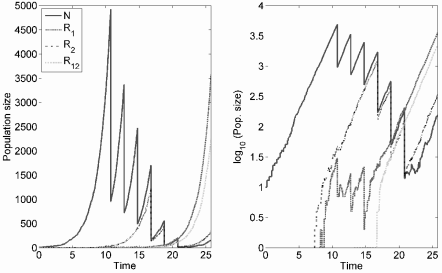
Example realization of treatment under the stochastic Day model using a simple birth-death process. Three treatments of the weak drug are followed by three of the strong; parameters are λ = 1.0, µ = 0.4, α1 = α2 = 0.001. These are chosen so that the granularity of the stochastic process can be displayed, and resistance emerges in an unrealistically small tumor.
9.5.3.4 Goldie-Coldman contra Norton-Simon
The Goldie-Coldman and Norton-Simon models are somewhat at odds in their predictions for optimizing therapy. Goldie-Coldman attempts to minimize the emergence of new resistance during the treatment period by alternating drugs. As also discussed in Section 9.4.5, the Norton-Simon model prescribes sequential dose-dense therapy, under the implicit premise that clinically relevant heterogeneity in drug sensitivity is already present when treatment is initiated. Indeed, the Goldie-Coldman model itself predicts that drug resistance arises very early in a tumor’s natural history.
Several clinical trials have tested alternating therapy versus standard chemotherapy for breast cancer [10, 17], but all have failed to demonstrate any benefit to alternating over standard schedules. The CALGB 9741 trial [14] is the major trial supporting dose-density, although it does not address sequential versus alternating therapy. Several other trials evaluated sequential versus concurrent or alternating therapy, and seem to suggest a slight benefit to sequential therapy. For example, Bonadonna et al. [11] found sequential DOX → CMF schedule superior to alternating DOX/CMF. However, CMF → DOX was no better than standard CMF, suggesting a simple “sequential is better” interpretation is not really correct, and the order in which these particular agents are administered matters.
A problematic argument based on kinetic resistance suggests that sequential therapy should be generally superior to alternating schedules. Assume that a tumor is evenly divided between two subpopulations, each of which is sensitive to only one of two agents. Then alternating the two agents might be expected to increase kinetic resistant since individual subpopulations would have more time to regrow between treatments. However, if growth rate is modulated by the total tumor population and not the size of any single subpopulation, then the overall response of each subpopulation will be similar whether drugs are alternated or given sequentially, assuming each is equally effective against the sensitive subpopulation.
From this, we argue that, while the clinical data lends more support to the Norton-Simon approach over the Goldie-Coldman, there is no fundamental conflict between the two models. Rather, the conflict arises because the dichotomy between treatment strategies that focus on dose-density vs. those that focus on alternating (or concurrent) treatment are clinically incompatible. The data suggests that maximizing dose-density is more important.
9.5.4 The Monro-Gaffney model and palliative therapy
In the previous two sections we discussed the most influential models in modern clinical oncology. In particular, the log-kill model and the Norton-Simon hypothesis have helped motivate a treatment model where therapy is given as soon as possible in a relatively brief, intense period. Under the Norton-Simon model, an intensive dose-dense regime yields the lowest cancer cell nadir and consequently the best chance for cure. However, as we shall see, when reasonable hope for a cure cannot be entertained, lower-dose, long-term therapy may better increase survival time.
9.5.4.1 The model
Recently, Monro and Gaffney [51] proposed a relatively simple dynamical model that combines the Norton-Simon and Goldie-Coldman notions—that is, the model assumes that chemotherapy efficacy and per-unit time probability of a resistance mutation are both proportional to the unperturbed Gompertzian tumor growth rate. One drug and two classes of cells—drug-sensitive (S) and resistant (R)—are considered. Let, at time t,
NS(t) = number of chemosensitive cells, and
NR(t) = number of cells with complete resistance to the drug:
The total number of cells in the tumor is therefore N(t) = NS(t) + NR(t). Both classes proliferate via identical Gompertzian kinetics and mutate between class. Mutation from the sensitive to the resistant class occurs at rate τ1 per cell cycle, and back mutations occur at rate τ2 per cell cycle. These considerations give the following model:
dNSdt=βln(N∞N)[NS+τ2NR−τ1NS−λCNS], (9.90)
dNRdt=βln(N∞N)[NR+τ1NS−τ2NR]. (9.91)
The first term in both equations gives Gompertzian growth modulated by the total cell count. The per-capita growth rate is β ln(N∞/N), and this term governs the rates of mutation between the classes and the response to treatment. From this it follows that τ1 and τ2 are mutation rates per cell cycle, rather than simply per unit time. The term −λC NS represents the death rate of sensitive cells in response to some concentration of the drug, C, which is also proportional to the proliferation rate. We can also lump λC into a single parameter, C0.
This model represents an explicit union of the two most influential cancer treatment models, and it is simple but potentially powerful framework with which we can evaluate the Norton-Simon notion of dose-density while explicitly taking Goldie-Coldman into account. Moreover, it would be a straightforward exercise to expand this model to consider the effects of two non-cross-resistant drugs and determine if the Goldie-Coldman prediction that drugs should be rapidly alternated is preserved when Norton-Simon is taken into account. These are important and straightforward projects, but Monro and Gaffney turned their attention toward the problem of maximizing survival in the setting of palliative chemotherapy, rather than maximizing cure probability by minimizing cell nadir or the probability of a resistant mutant arising.
9.5.4.2 Predictions of the Monro-Gaffney model
Optimal dose. Monro and Gaffney hypothesized that overly aggressive treatment in a palliative setting could accelerate selection of treatment resistant mutants and therefore ultimately decrease response to therapy and survival. Numerical simulation of the model indeed supports this suggestion. This is because resistance emerges quickly in response to high-dose therapy, leading to treatment failure no matter how much chemotherapy is given. However, an overly low dose does not sufficiently inhibit sensitive cells, and survival is also decreased. The optimum dose suppresses sensitive cells, but not so much that resistant cells have a strong survival advantage. This is summarized in Figures 9.11 and 9.12.
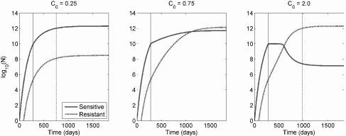
Response to therapy for three different levels of continuous chemotherapy under the Monro-Gaffney model. The solid vertical line indicates the start of therapy, and the dotted line is the expected time of death. Too little therapy, and the growth of sensitive cells is not sufficiently suppressed (left panel), but too much promotes the rapid overgrowth of resistant cells (right panel). The optimal level, shown in the center panel, leads to a rough balance between sensitive and resistant cells. Parameter values are N∞ = 2 × 10¹², β = 5.928 × 10⁻³ day−1, τ1 = τ2 = 10−6. Death is assumed to occur at a total tumor burden of 5 × 10¹¹ cells, and treatment is initiated when N = 1010 cells.
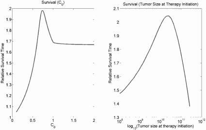
The left panel gives relative survival time (survival time under treatment / survival time without treatment) for continuous chemotherapy following initiation at a tumor size of 1010 cells under different values of C0, representing the strength of chemotherapy. The right panel gives relative survival time when therapy is initiated at different tumor burdens with a fixed C0 = 0.75.
Treatment delay. A second interesting result of the Monro-Gaffney model is its suggestion that a moderate treatment delay can improve survival time, as shown in Figure 9.12. This is corroborated by results for the clinical treatment of some slow-growing, chronic cancers, in which no survival advantage is conferred by initiating treatment earlier. For example, chronic lymphocytic leukemia (CLL) is incurable but is characterized by a long, indolent clinical course. Early treatment offers no survival benefit in this disease, and therapy is generally deferred until there is clear evidence of disease progression [38].
A large study [48] found, in accord with other results, that androgen deprivation therapy for localized, low-risk prostate cancer actually decreased cancer-specific survival (although it did not affect overall survival). The authors suggested one possible explanation:
Suppression of moderately or well-differentiated cells not destined to harm a patient’s overall survival may allow for the establishment or overgrowth of more rapidly growing malignant clones.
While this study examined hormonal treatment for prostate cancer, the results of the Monro-Gaffney model are likely generalizable to it.
The results in [48] also highlight one aspect of drug resistance that we have not yet taken into account in a model: resistance can be achieved by fairly general mechanisms such as increased proliferation rate or reduced apoptosis, which are expected to translate into a more aggressive phenotype. We also note that, under the model, the longer therapy is delayed, the greater the optimum level of chemotherapy.
Dose-density. Monro and Gaffney also studied non-continuous dosing computationally, and found that protracted dose-densification and intensification schemes generally decrease survival time in the palliative setting, which is unsurprising given the results for continuous therapy. However, they noted that brief dose-dense schemes for “marginally curable” tumors may give an increased chance of cure and minimally affect survival time, and therefore may be appropriate for potentially curable cancers.
9.5.4.3 Summary
The Norton-Simon and Goldie-Coldman models predict that, to maximize probability of a cure, therapy should be initiated as soon as possible and be as dose-dense as possible. That is, “hit ’em hard and fast.” The Goldie-Coldman model and variations of it make further predictions about the alternating or sequential scheduling of agents. This is when the goal of therapy is to eliminate all cancer cells from the body. Sadly, for most advanced or metastatic solid tumors, curative therapy remains elusive, and the job of the medical oncologist is largely to provide palliative care, using chemotherapy to extend life or reduce tumor-related symptoms, but not to cure. In this case the Monro-Gaffney model suggests the “less-is-more” approach just discussed. We note that the role of chemotherapy toward the end of life is a complex emotional and sociological issue, and the reader may consult [37] for an introduction to this perplexing but important subject.
At least some data supports the notion that less aggressive therapy in the palliative setting is superior. Palliative chemotherapy has clearly been shown to extend survival in many malignancies [37], but beyond first- or second-line chemotherapy the benefit is less clear. In the case of non-small cell lung cancer (NSCLC), one study [49] found the response rate to third- or fourth-line therapy to be 2.3% and 0%, respectively. The deleterious effect of aggressive therapies on the failing physiologies of terminal cancer patients also doubtless plays a role in the influence on survival, either positive or negative, of chemotherapy given near the end of life. Von Gruenigen et al. [32] found that aggressiveness of care near the end of life in ovarian cancer patients was associated with lower survival, as was chemotherapy during the last three months of life. Hospice care, which forgoes any attempt at curative chemotherapy or other aggressive treatments, was associated with longer survival compared to non-hospice care for certain terminally ill cancer patients [15]. These results are likely more related to the effect of aggressive therapy on the patient rather than any effect on tumor biology.
9.5.5 The role of host physiology
We have exclusively focused on the effect of chemotherapy on cancer cells, but we must at least note the importance of host physiology, as toxicity to healthy tissues is dose-limiting in cancer therapy, and also can have a detrimental effect on survival. Several authors have considered bone marrow suppression, the most common toxicity. Panetta, for example, considered this in a very simple context [56], while Scholz et al. [61] have proposed a complex model for granulopoiesis, suppression by chemotherapy, and exogenous granulocyte colony-stimulating factor (G-CSF, a growth factor promoting granu-lopoiesis) support.
9.6 Heterogeneous populations: The cell cycle
A number of models have examined treatment on a tumor with sensitive and resistant populations where sensitivity is determined (at least partly) by whether the cell is quiescent or passing through the cell cycle. Therefore, we turn our attention to the cell cycle and how it influences resistance to and scheduling of chemotherapy.
9.6.1 The Smith-Martin conceptual model
It is worthwhile to take this opportunity to explicitly present the cell cycle and some models of the process. The cell cycle classically consists of four phases: G1 (Gap 1), S (Synthesis), G2 (Gap 2), and M (Mitosis). In G1, the cell increases in size while proteins necessary for DNA synthesis are produced. DNA replication occurs in S phase. The cell is readied for mitosis in G2, and the DNA is divided between two daughter cells in M phase. Interphase comprises G1, S, and G2. Chemotherapy generally acts on actively cycling cells, and a number of agents primarily or only affect cells in particular phases. For example, mitotic inhibitors such as the taxanes and vinca alkaloids are G2/M phase-specific, while antimetabolites like methotrexate inhibit DNA synthesis and are therefore specific for S phase. Cells that are not actively passing through the cycle are sometimes said to be in G0, which may be considered a precursor or extension of G1.
Smith and Martin proposed a conceptual kinetic model for cell proliferation in a classic 1973 paper, “Do Cells Cycle?” [65]. They proposed that following mitosis cells enter some state (A) in which they remain for a variable length of time, but exit with a constant probability, P. That is, the time until exit is an exponential random variable, and in a continuous model the rate of exit is first-order with respect to A-state cells. On leaving A-state, cells enter B-phase, which lasts a fixed amount of time, TB, and represent passage through the cell-cycle. Following mitosis, cells re-enter the A-state. Thus, the aggregate growth rate of a cell population is a function of the probability (i.e. exponentially distributed rate) at which cells exit A-state, the length of B-phase, and the cellular death rate. For the interested reader, Smith and Martin [65] present equations with which P can be explicitly determined from the gross cell growth rate and TB. The model is illustrated schematically in Figure 9.13.
![Figure showing schematic of the conceptual kinetic model for cell proliferation proposed by Smith and Martin (see also Figure 1 of [65]).](http://imgdetail.ebookreading.net/math_science_engineering/24/9781498785532/9781498785532__introduction-to-mathematical__9781498785532__image__fig9-13.png)
Schematic of the conceptual kinetic model for cell proliferation proposed by Smith and Martin (see also Figure 1 of [65]).
Smith and Martin also noted that, if the cell cycle were a fixed-length process and all cells were committed to cycling, then cells starting from the same point in the cell cycle should divide in synchrony. This prediction can be tested by labeling cells with a pulse of [3H]dT (radio-labeled Thymidine, a component of DNA). Only cells in S phase will pick up the label, so in a culture with cells in various stages of the cycle, a single cohort can be marked. If cells progress through the cell cycle together, then this cohort will all divide at the same time, and no non-labeled cells will divide at that time (because unlabeled cells must have been in a different portion of the cell cycle when the label was applied and would therefore enter mitosis at a different time if the cell cycle were of unvarying length for all cells). In such experiments, one can measure, at any given moment, what fraction of cells undergoing mitosis are labeled (in the marked cohort). This measure is called the fraction of labeled mitoses, or FLM. So, if the cell cycle length were invariant, then the FLM would either be 100% (the cohort is in mitosis) or 0% (the cohort is in interphase). Therefore, the FLM as a function of time would (ideally) be a Heaviside function, jumping instantly to 1 when the cohort entered mitosis and dropping instantly to 0 as the cohort leaves mitosis. This pattern is observed to some degree in actual experiments; however, over time successive peaks or jumps are dampened; i.e., they become more spread out until eventually the FLM approaches an equilibrium proportion between 0 and 1. Smith and Martin explained this dampening by suggesting that the time spent in the A-phase varies among cells, and their model predicted that the dampening in the FLM oscillations should be exponential. This result generally agrees well with experiment. The period of the oscillations are not affected by P (the probability a cell exits the A-state), but the rate of dampening is.
9.6.2 A delay differential model of the cell cycle
The Smith-Martin model translates perfectly into a delay differential equation. Suppose we have a class of cells in the A-state—i.e., they are non-cycling, quiescent, or in G0. Let Q(t) be the number of these quiescent cells. The number of actively cycling B-state cells, on the other hand, we denote P(t). We assume that cells transition from quiescent to cycling states at constant rate k, taking exactly τ units of time to complete the cell cycle. Following passage through the cell cycle, each cell gives rise to two daughter cells that re-enter the quiescent compartment. Disregarding cell death for the moment, we can express this biology with the following model:
dQ(t)dt=−kQ(t)+2kQ(t−τ), (9.92)
dP(t)dt=kQ(t)−kQ(t−τ), (9.93)
with appropriate initial conditions. This basic model can be extended to include details of the cell cycle. For example, one can subdivide the cycling cell class (P(t)) into number of cells in interphase, say I(t), and number in mitosis, M(t). Furthermore, define τ0 and τ1 to be the time it takes to pass through interphase and mitosis, respectively. Ignoring death again gives
dQ(t)dt=−kQ(t)+2kQ(t−τ0−τ1), (9.94)
dI(t)dt=kQ(t)−kQ(t−τ0), (9.95)
dM(t)dt=kQ(t−τ0)−kQ(t−τ0−τ1), (9.96)
again with appropriate initial conditions. This slightly more complicated model agrees extremely well with the dynamics predicted by Smith and Martin. Starting with a population of quiescent cells at time 0 with all other variables and history set to 0, we observe damped oscillations in the number of cells in mitosis (as well as interphase and quiescence; Figure 9.14). Moreover, as predicted, these oscillations are characterized by a rapid rise to a peak followed by exponential decline. For smaller k (slower transition from quiescence to the cell cycle), oscillations are damped more quickly, which was also predicted by Smith and Martin. Following an early period of irregular growth with oscillations in the different compartments, there is fairly rapid convergence to a constant distribution of cells among states and exponential growth (Figure 9.14). Genrally, dynamics of this and the simpler model that considers only P and Q are similar.
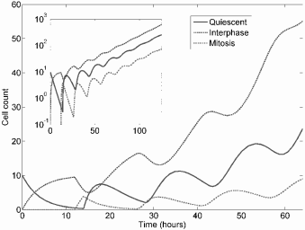
Basic dynamics of a delay model for the cell cycle considering quiescence, interphase, and mitosis derived from Smith and Martin’s conceptual model. The insert shows the dynamics on a log-scale and demonstrates that the model converges to exponential growth.
Having formulated a basic model that gives realistic dynamics, we now introduce cell cycle-specific treatment to this framework. First we consider a treatment that targets only actively cycling cells with the simpler formalism. Suppose drug efficacy (cell-kill rate, δ) is proportional to concentration, C(t), and suppose C(t) is piecewise constant—i.e., either chemotherapy is present at a constant dose or it is not present at all. Our model then becomes the following:
dQ(t)dt=−kQ(t)+2kQ(t−τ)e−δ∫tt−rC(s)ds, (9.97)
dP(t)dt=kQ(t)−kQ(t−τ)e−δ∫tt−rC(s)ds−δC(t)P, (9.98)
(9.99)
C(t)={C0(treatment on),0(treatment off).
With this model one can examine how an exponentially growing tumor responds to cell cycle-specific drugs while explicitly accounting for age structure. During the period of time in which the drug is administered, t ∈ [0, T], the drug concentration, measured as area under the curve (AUC), is
AUC=∫T0C(s)ds=constant. (9.100)
We use two metrics when evaluating drug efficacy: (1) tumor size at the end of treatment, and (2) tumor size after some large time, Tmax. The former is similar to cell nadir but accounts for positive growth during treatment time, and the latter is a surrogate for survival time. Note that tumor size after T is not a reliable marker for long-term response because of perturbations in age-structure. The basic dynamics of response to treatment for several simple infusion schedules are shown in Figure 9.15.
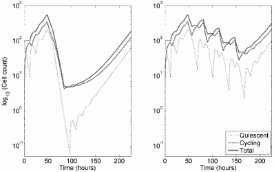
Time-series of tumor response to either one bolus infusion of chemotherapy or the same dose divided between four episodes.
According to this model, if the same cumulative dose is delivered in a single constant infusion, it is universally better to prolong the infusion time (Figure 9.16). Also, increasing the concentration of chemotherapy for a single infusion of fixed time gives diminishing returns with increasing dose, comparable to the plateau in cytotoxicity discussed in the section of dose-response curves.
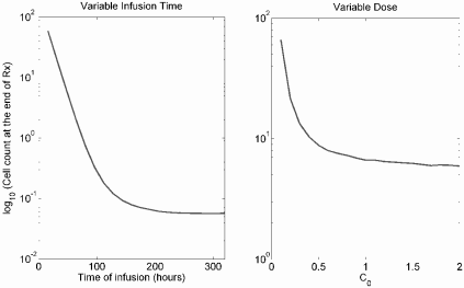
This figure demonstrates that the same dose delivered over a long time dramatically improves response, but the efficacy eventually plateaus. Increasing the dose delivered in a fixed time also results in increasing cytotoxicity that plateaus with increasing dose due to depletion of the sensitive cell population.
Numerical investigations reveal that dividing a single treatment into multiple treatments delivered in the same net amount of infusion time gives results that vary with cell proliferation rate, k, and with the drug’s efficacy, δ. In general, the cell nadir is lowest when a single treatment is given, an unsurprising result as this scenario represents the most dose-dense option. (See the discussion of the Norton-Simon model above.) However, dividing the dose into many treatments, while typically increasing cell nadir, can also increase survival time, unlike the basic Norton-Simon model. However, the picture is not that simple. In certain regions of parameter space, a smaller number of longer treatments is inferior to more, shorter treatments, especially in the case of a rapidly growing tumor (large k) or a strong drug (large δ). Thus, the model suggests that for highly responsive tumors either very few treatments or very many treatments should be given. The former should be done if the curative therapy is the goal, the latter if one is attempting to maximize survival. We leave confirmation of these results as an exercise.
9.6.3 Age-structured models for the cell cycle
Now we return our attention to age-structured models (see Chapter 4). The basic model for quiescent and cycling cells we studied above is in fact equivalent to an age structured partial differential equation (PDE) model, as we now demonstrate. Recall that P(t) is the number of cells in the cycling compartment. Cells enter this compartment at rate kQ(t) and complete division in exactly τ units of time. We let
p(t, a) = The population density of proliferating cells of age a, a ∈ [0, τ].
This is the density of cells of age a, the integral of which gives us number of cells. Now, we have that cycling cells suffer mortality at rate δC(t) at time t. This gives us an advection PDE describing the passage of cells through time and age:
∂p∂t=−∂p∂a−δC(t)p(t,a). (9.101)
We impose boundary conditions at age 0 and age τ as:
p(t,0)=kQ(t)andp(t,τ)=kQ(t−τ)exp(−δ∫tt−rC(s)ds). (9.102)
To complete the model, we include the governing equation for Q(t),
dQ(t)dt=−kQ(t)+2kQ(t−τ). (9.103)
To see that the age-structure model is equivalent to the delay differential model, we integrate over age to get the number of cycling cells at time t:
P(t)=∫τ0p(t,s)ds. (9.104)
Integrating (9.101) from 0 to τ with respect to age a yields
dP(t)dt+p(t,τ)−p(t,0)=−δC(t)P(t). (9.105)
Applying the boundary conditions defined in (9.102) returns us to the expression for dP(t)/dt in (9.99):
dP(t)dt=kQ(t)−kQ(t−τ)exp(−δ∫tt−τC(s)ds)−σC(t)P(t). (9.106)
A number of authors have proposed various age-structured models of the cell cycle for tumor cells and their response to cell cycle-specific chemotherapy. Spinelli et al. [66] proposed a model for proliferating and quiescent cells somewhat similar to that above. Basse et al. proposed several models for the cell cycle in tumor cells which explicitly consider multiple stages of the cell cycle [2, 3, 4]. However, in these models cells cycle continuously with no quiescent state (A-state). The most general formulation is given in [4].
Gaffney [25, 26] also proposed several age-structured models that considered mutation to resistance, as in the Goldie-Coldman model, and used these models to study the scheduling of S-phase specific chemotherapies.
A number of models have also been proposed for the response of cycling cells to continuous low-dose irradiation, including several age-structured models [13, 35, 36, 69]. For example, Chen et al. [13] proposed a similar model to that studied above. Letting n(t, a) represent the population density of cells with age a, a ∈ [0, ∞), we have the model,
∂n∂t=−∂n∂a−˙Dα(a)n−g(a)n, (9.107)
where Ḋ is the radiation dose-rate, α(a) gives first order killing that depends upon cell age, and hence position in the cell cycle, and g(a) represents the rate at which cells of age a produce two daughter cells of age 0. The daughters immediately re-enter the cell cycle with no quiescent phase. The domain here is semi-infinite, as cells exit the cycle according to the age-dependent probability distribution g(a) and no right boundary condition is imposed. On the left boundary, however,
n(0,t)=2∫∞0g(s)n(s,t)ds. (9.108)
While this model was meant to represent continuous irradiation, it is equivalent to the case of continuous chemotherapy we consider above. Note that this model ignores any cell death that is quadratic with the dose (as in the linear-quadratic model) or repair of sublethal damage; such models are discussed more extensively in Chapter 11. Similar to our conclusion using the delay model, the model of Chen et al. [13] and later extensions by Hahn-feldt and Hlatkey [35, 36] suggest that protracted irradiation schedules may kill cells better than more intense irradiation. However, intracellular DNA repair/misrepair dynamics of radiation-induced lesions imply that shorter irradiation times lead to greater cell death (again, discussed in Chapter 11). Thus, cell cycle redistribution and DNA repair are competing intracellular dynamics that determine optimal treatment time.
This last point highlights the very important observation that applies to chemotherapy. The pharmacokinetics of the drug in plasma, delivery to the target tumor site, cellular uptake, detoxification, and repair of intracellular lesions will affect optimal treatment in a way that cannot be simply accounted for with first-order cell killing.
9.6.4 More general sensitivity and resistance
Many other models designed to study sensitive and resistant tumor cell populations use simpler ODE formulations for the cell cycle or for transfer between quiescent and proliferating compartments. One of the earliest was that of Birkhead et al. [9], who considered proliferating and quiescent cells which were either genetically susceptible or resistant to some chemotherapy. Let SP(t) and SQ(t) represent the number of proliferating and quiescent cells that are sensitive to the drug, respectively. Similarly, let RP(t) and RQ(t) be the amount of proliferating and quiescent resistant cells, respectively. Cells transition between quiescent and cycling states at constant per-capita rates, and sensitive cells mutate to become resistant at rate c per cell division. Only genetically susceptible cells that are actively proliferating are vulnerable to chemotherapy. This leads to Birkhead et al.’s formal model:
dSPdt=αSP−ηSPμSP−μSP−∈SP+λSQ, (9.109)
dSQdt=μSP−λSQ, (9.110)
dRPdt=∈SP+αRP−ηRP−μRP+λRQ, (9.111)
dSQdt=μSP−λSQ. (9.112)
This is a basic ODE framework in which the notions of cell cycle specifity considered in the previous section may be combined with mutation to resistance as in the Goldie-Coldman models.
Panetta and Adam [55] later considered a model for cell cycle specific chemotherapy essentially identical to that of Birkhead et al., but without a class of resistant cells. Hahnfeldt et al. [34] also used a similar framework to study two types of proliferating cells, with transitions between compartments, that are differentially sensitive to treatment.
These models tend to agree that intense treatment yields diminishing returns as treatment-sensitive cells become depleted. Hahnfeldt et al. concluded that long term, low dose, “metronomic” therapy may be a better strategy to suppress tumor growth in the long term rather than trying to destroy all cells in the short term.
9.7 Drug transport and the spatial tumor environment
The deranged tumor microenvironment represents a significant barrier to drug transport into the tumor, which can become another mechanism generating treatment resistance. In this section we present some basic transport principles, and then mention how these concepts relate to the tumor spheroid, and tumor cord, geometries (see Chapter 3).
9.7.1 Solute transport across tumor capillaries
Solute exchange between the vascular and extravascular spaces is governed by diffusion and convection. Specifically, exchange is determined by transcap-illary concentration gradient, the hydrostatic and osmotic pressure gradients, vascular surface area for exchange, A (mm2), and three key transport parameters: the hydraulic permeability (or hydraulic conductivity) Lp (mm / hr / mmHg), the diffusional permeability P (mm / hr), and the osmotic reflection coefficient σ (unit-less) [39]. The reader may consult the 1987 review by Jain [39] for an extensive discussion of transcapillary transport in tumors.
Consider the concentration of some solute, S, in a small section of capillary. According to Starling’s hypothesis, fluid flow across the capillary wall, JF, is
JF=LpA[PV−PE−σ(∏V−∏E)]. (9.113)
Here, PV − PE (mmHg) is the hydrostatic pressure difference, and ΠV − ΠE (mmHg) is the osmotic pressure difference.
The total flow of solute, JS, in units of mass per time (mg / hr), from plasma into the tumor extracellular space occurs by passive diffusion and convective transport across the capillary wall according to the Staverman-Kedem-Katchalsky equation [39]:
JS=PA(SV−SE)︸diffusion+JF(1−σF)ΔSlm︸convection, (9.114)
ΔSlm=SV−SEln(SV/SE), (9.115)
where SV is the solute concentration (mg / mm3) on the vascular side of the capillary, and SE is the concentration on the extracellular side. Therefore, ΔSlm is the solute log-mean concentration difference. The first term in equation (9.114) gives transport by diffusion, and the second is transport by convection. Constants P and A are defined above.
Another key transport parameter, the hydraulic permeability Lp, is defined as the flow of water through a unit area of capillary wall per unit difference in hydrostatic pressure across the wall [50]. The diffusional permeability P is the mass transport of the solute per unit area of capillary wall per unit of solute concentration difference when the fluid flow is zero [50].
The osmotic pressure is determined by the molarity of dissolved solutes in solution; i.e., Π ∝ M RT, where M is molarity, R is the universal gas constant, and T is temperature. The osmotic pressure gradient across the capillary wall induces fluid flow. The osmotic reflection coefficient σ can be thought of as the fraction of solute that is “reflected” at the capillary wall during ultrafiltration, as opposed to that which flows freely across [50]. Only the fraction reflected can exert osmotic pressure. The value of σ depends, in part, on size of the solute; it is close to 1 for macromolecules such as albumin, and closer to 0 for micromolecules.
The solvent-drag reflection coefficient, σF , measures the coupling between fluid flow and solute flow [39]. If σF is small, then the solute is readily transported by fluid flow. For a given substance the solvent-drag reflection coefficient, σF , tends to be similar in value to the osmotic reflection coefficient, σ [19].
Another important ratio is the Peclet number (Pe):
Pe=JF(1−σF)PA=Lp(1−σF)P[(PV−PE)−σ(∏V−∏E)]. (9.116)
The Peclet number indicates the relative importance of diffusive versus convective transport [39]. If Pe is small, which tends to be the case for mi-cromolecules, then diffusive transport is dominant. In this case, JS can be approximated using an effective permeability coefficient PEff, as follows:
JS=PEffA(SV−SE). (9.117)
In tumors, the intercapillary distance is typically much greater than normal tissue, hampering drug delivery. Moreover, blood flow is heterogenous and vessels are prone to collapse, causing heterogeneity in delivery. The vas-culature is malformed, immature, and quite leaky. This fact allows a great deal of fluid extravasation into the tumor and leakage of macromolecules, giving high hydrostatic and osmotic pressure in the tumor interstitium. Thus, the hyrdostatic pressure and osmotic pressure differences are minimal. On the other hand, the diffusional permeability, P, and hydraulic conductivity, LP, are much higher in leaky tumor vessels compared to normal, well-formed capillary beds.
9.7.2 Fluid flow in tumors
Flow through the tumor interstitium may be modeled by Darcy’s law for flow in a porous medium, which gives volumetric flow rate, Q (mm3 / hr), as:
Q=−AK∇P, (9.118)
where A (mm2) is the cross-sectional area of flow, K (mm2 / mmHg / hr) is the hydraulic conductivity of the medium, and ∇P is the interstitial pressure gradient. Dividing by A gives the flux (or “Darcy flux”), u:
u=−K∇P. (9.119)
We also have the continuity equation for fluid flow:
dρdt+∇⋅(ρu)=ϕ(x), (9.120)
where ρ is density and ϕ is the source/sink term (in units of volumetric flow per unit volume of tissue). In the case of an incompressible fluid, this reduces to:
∇⋅u=ϕ(x). (9.121)
Combining equations (9.119) and (9.121) gives:
∇⋅(−K∇P)=ϕ(x). (9.122)
Baxter and Jain applied these basic equations to describe fluid flow in a tumor spheroid [5], and also describe interstitial solute flow in the spheroid by a convection-diffusion equation.
Volumetric flow through a capillary is proportional to the product of the hydrostatic pressure drop from the arterial to the venous ends of the capillary and the resistance to flow [40]; that is,
Q=ΔPFR. (9.123)
In the case of laminar fluid flow in a cylinder of length L and radius R the Hagen-Poiseuille law gives flow resistance as:
FR=8ηLπR4. (9.124)
Pozrikidis and Farrow [58] further describe fluid flow in a tumor at the mi-crovessel level.
9.7.3 Tumor spheroid
The tumor spheroid geometry has been widely used to model delivery of cytotoxic drugs. A series of papers by Baxter and Jain [5, 6, 7] modeled fluid flow and macromolecule (e.g. antitumor monoclonal antibodies) delivery to tumors using the spheroid as the base geometry. One of the most important results is that tumors have high interstitial fluid pressure in the core, but this pressure drops off in the periphery. This causes radially outward fluid flow and convective transport of macromolecules out of the tumor. Also, continuous or divided drug infusions can better maintain a transcapillary solute gradient.
9.7.4 Tumor cord framework
The other major geometry that has been used to model in vivo tumors is the tumor cord. Tumor cords are one of the fundamental microarchitectures of solid tumors, consisting of a microvessel nourishing nearby tumor cells [8]. This simple architecture has been used by several authors to represent the in vivo tumor microenvironment [8, 19, 67], and a whole solid tumor can be considered an aggregation of a number of tumor cords.
Doxorubicin (DOX), an important and potent antitumor agent, is characterized by poor penetration into the tumor mass. Eikenberry [19] extended a previous model by El Kareh and Secomb [21], which modeled DOX plasma pharmacokinetics (using a three-compartment model by Robert et al. [59]) and diffusional transport into a non-spatial tumor, to consider transport into a tumor cord geometry using the solute transport laws discussed above.
9.8 Exercises
Exercise 9.1: Consider two exponentially expanding populations of cells, one treated, NT , and one a control, NC. Assume the treatment population is exposed to a constant concentration of drug, C, and exposure induces death at the per capita rate β per unit of drug. Show that for a total exposure time T, we arrive at the log-linear model:
S=NTNC=e−βC×T (9.125)
Exercise 9.2: We do not arrive at a simple log-kill model if the underlying cellular growth dynamic is not exponential. Consider the case of logistic growth:
dNCdt=αNC(1−NCK) (9.126)
dNtdt=αNT(1−NTK)−βCNT. (9.127)
1. Find the analytic solution to the system and confirm that for constant C the surviving fraction can be expressed as:
S=NTNC=e−αT(K−N0)(β0+α)+N0(β0+α)eT(β0−α)(Kβ0+Kα−N0β0)+N0β0 (9.128)
where we let β0 = βC.
2. Find conditions on the parameters for a log-kill model to approximate survival, i.e. when:
S≈e−βC×T=e−β0T (9.129)
Why are these conditions unsurprising?
3. Reproduce Figure 9.2, which plots S versus either β0 or T on a semi-logarithmic scale. These plots demonstrate a shoulder region when concentration is varied and a roughly bi-exponential curve when exposure time is varied. This suggests non-exponential cell growth as a possible explanation for departures from the log-kill model.
Exercise 9.3: Norton and Simon assume that the tumor growth fraction is equivalent to the per-capita growth rate, bln(N∞N(t))
Exercise 9.4: Apply the general Norton-Simon model, dN/dt = GF(N)N(t) − L(t)GF(N)N(t), to different basic growth laws for tumor-growth, e.g. exponential, logistic, or von Bertalanffy. Determine which model predictions are preserved for sigmoidal growth versus the simple exponential growth.
Exercise 9.5: So far, we have only considered a constant level of chemotherapy that is either on or off. Implement 1−, 2−, and 3−compartment pharmacokinetics models for chemotherapy into the model. Parameterized 2- and 3-compartment models for the agent doxorubicin can be found in [20, 31, 59]. Do more realistic pharmacokinetics change the qualitative predictions?
References
[1] Adams DJ: In vitro pharmacodynamic assay for cancer drug development: application to crisnatol, a new DNA intercalator. Cancer Res 1989, 49:6615–20.
[2] Basse B, Baguley BC, Marshall ES, Joseph WR, van Brunt B, Wake G, Wall DJ: A mathematical model for analysis of the cell cycle in cell lines derived from human tumors. J Math Biol 2003, 47:295–312.
[3] Basse B, Baguley BC, Marshall ES, Joseph WR, van Brunt B, Wake G, Wall DJ: Modelling cell death in human tumour cell lines exposed to the anticancer drug paclitaxel. J Math Biol 2004, 49:329–57.
[4] Basse B, Ubezio P: A generalised age- and phase-structured model of human tumour cell populations both unperturbed and exposed to a range of cancer therapies. Bull Math Biol 2007, 69:1673–90.
[5] Baxter LT, Jain RK: Transport of fluid and macromolecules in tumors. I. Role of interstitial pressure and convection. Microvasc Res 1989, 37:77– 104.
[6] Baxter LT, Jain RK: Transport of fluid and macromolecules in tumors.
II. Role of heterogeneous perfusion and lymphatics. Microvasc Res 1990, 40:246–63.
[7] Baxter LT, Jain RK: Transport of fluid and macromolecules in tumors. III. Role of binding and metabolism. Microvasc Res 1991, 41:5–23.
[8] Bertuzzi A, D’Onofrio A, Fasano A, Gandolfi A: Regression and regrowth of tumour cords following single-dose anticancer treatment. Bull Math Biol 2003, 65:903–931.
[9] Birkhead BG, Rankin EM, Gallivan S, Dones L, Rubens RD: A mathematical model of the development of drug resistance to cancer chemotherapy. Eur J Cancer Clin Oncol 1987, 23:1421–1427.
[10] Boccardo F, Rubagotti A, Amoroso D, Perrotta A, Sismondi P, Farris A, Mesiti M, Gallo L, Pacini P, Villa E, Agostara B: Lack of effectiveness of adjuvant alternating chemotherapy in node-positive, estrogen-receptor-negative premenopausal breast cancer patients: Results of a multicentric Italian study. The Breast Cancer Adjuvant Chemo-Hormone Therapy Cooperative Group (GROCTA). Cancer Invest 1997, 15:505–512.
[11] Bonadonna G, Zambetti M, Moliterni A, Gianni L, Valagussa P: Clinical relevance of different sequencing of doxorubicin and cyclophosphamide, methotrexate, and Fluorouracil in operable breast cancer. J Clin Oncol 2004, 22:1614–1620.
[12] Bonilla L, Ben-Aharon I, Vidal L, Gafter-Gvili A, Leibovici L, Stemmer SM: Dose-dense chemotherapy in nonmetastatic breast cancer: A systematic review and meta-analysis of randomized controlled trials. J Natl Cancer Inst 2010, 102:1845–1854.
[13] Chen PL, Brenner DJ, Sachs RK: Ionizing radiation damage to cells: Effects of cell cycle redistribution. Math Biosci 1995, 126:147–170.
[14] Citron ML, Berry DA, Cirrincione C, Hudis C, Winer EP, Gradishar WJ, Davidson NE, Martino S, Livingston R, Ingle JN, Perez EA, Carpenter J, Hurd D, Holland JF, Smith BL, Sartor CI, Leung EH, Abrams J, Schilsky RL, Muss HB, Norton L: Randomized trial of dose-dense versus conventionally scheduled and sequential versus concurrent combination chemotherapy as postoperative adjuvant treatment of node-positive primary breast cancer: First report of Intergroup Trial C9741/Cancer and Leukemia Group B Trial 9741. J Clin Oncol 2003, 21:1431–439.
[15] Connor SR, Pyenson B, Fitch K, Spence C, Iwasaki K: Comparing hospice and nonhospice patient survival among patients who die within a three-year window. J Pain Symptom Manage 2007, 33:238–426.
[16] Day RS: Treatment sequencing, asymmetry, and uncertainty: Protocol strategies for combination chemotherapy. Cancer Res 1986, 46:3876– 3885.
[17] De Placido S, Perrone F, Carlomagno C, Morabito A, Pagliarulo C, Lauria R, Marinelli A, De Laurentiis M, Varriale E, Petrella G, et al: CMF vs alternating CMF/EV in the adjuvant treatment of operable breast cancer. A single centre randomised clinical trial (Naples GUN-3 study). Br J Cancer 1995, 71:1283–1287.
[18] Drewinko B, Patchen M, Yang LY, Barlogie B: Differential killing efficacy of twenty antitumor drugs on proliferating and nonproliferating human tumor cells. Cancer Res 1981, 41:2328–2333.
[19] Eikenberry S: A tumor cord model for doxorubicin delivery and dose optimization in solid tumors. Theor Biol Med Model 2009, 6:16.
[20] Eksborg S, Strandler HS, Edsmyr F, Näslund I, Tahvanainen P: Phar-macokinetic study of i.v. infusions of adriamycin. Eur J Clin Pharmacol 1985 28:205–212.
[21] El-Kareh AW, Secomb TW: A mathematical model for comparison of bolus injection, continuous infusion, and liposomal delivery of Doxoru-bicin to tumor cells. Neoplasia 2000, 2:325–338.
[22] El-Kareh AW, Secomb TW: A mathematical model for cisplatin cellular pharmacodynamics. Neoplasia 2003, 5:161–169.
[23] El-Kareh AW, Secomb TW: Two-mechanism peak concentration model for cellular pharmacodynamics of Doxorubicin. Neoplasia 2005, 7:705– 713.
[24] Foster PL: Methods for determining spontaneous mutation rates. Methods Enzymol 2006, 409:195–213.
[25] Gaffney EA: The application of mathematical modelling to aspects of adjuvant chemotherapy scheduling. J Math Biol 2004, 48:375–422.
[26] Gaffney EA: The mathematical modelling of adjuvant chemotherapy scheduling: Incorporating the effects of protocol rest phases and phar-macokinetics. Bull Math Biol 2005, 67:563–611.
[27] Gilman A: The initial clinical trial of nitrogen mustard. Am J Surg 1963, 105:574–578.
[28] Goldie JH, Coldman AJ: A mathematic model for relating the drug sensitivity of tumors to their spontaneous mutation rate. Cancer Treat Rep 1979, 63:1727–1733.
[29] Goldie JH, Coldman AJ: Quantitative model for multiple levels of drug resistance in clinical tumors. Cancer Treat Rep 1983, 67:923–931.
[30] Goldie JH, Coldman AJ, Gudauskas GA: Rationale for the use of alternating non-cross-resistant chemotherapy. Cancer Treat Rep 1982, 66:439–449.
[31] Greene RF, Collins JM, Jenkins JF, Speyer JL, Myers CE: Plasma phar-macokinetics of adriamycin and adriamycinol: Implications for the design of in vitro experiments and treatment protocols. Cancer Res 1983, 43:3417–3421.
[32] von Gruenigen V, Daly B, Gibbons H, Hutchins J, Green A: Indicators of survival duration in ovarian cancer and implications for aggressiveness of care. Cancer 2008, 112:2221–2227.
[33] Gyllenberg M, Webb GF: Quiescence as an explanation of Gompertzian tumor growth. Growth Dev Aging 1989, 53:25–33.
[34] Hahnfeldt P, Folkman J, Hlatky L: Minimizing long-term tumor burden: The logic for metronomic chemotherapeutic dosing and its antiangio-genic basis. J Theor Biol 2003, 220:545–554.
[35] Hahnfeldt P, Hlatky L: Resensitization due to redistribution of cells in the phases of the cell cycle during arbitrary radiation protocols. Radiat Res 1996, 145:134–143.
[36] Hahnfeldt P, Hlatky L: Cell resensitization during protracted dosing of heterogeneous cell populations. Radiat Res 1998, 150:681–687.
[37] Harrington SE, Smith TJ: The role of chemotherapy at the end of life: “when is enough, enough?” JAMA 2008, 299:2667–2678.
[38] Hallek M, Cheson BD, Catovsky D, Caligaris-Cappio F, Dighiero G, Dhner H, Hillmen P, Keating MJ, Montserrat E, Rai KR, Kipps TJ; International workshop on chronic lymphocytic leukemia: Guidelines for the diagnosis and treatment of chronic lymphocytic leukemia. A report from the International Workshop on Chronic Lymphocytic Leukemia updating the National Cancer Institute Working Group 1996 guidelines. Blood 2008, 111:5446–5456.
[39] Jain RK: Transport of molecules across tumor vasculature. Cancer Metastasis Rev 1987, 6:559–593.
[40] Jain RK: Determinants of tumor blood flow: A review. Cancer Res 1988, 48:2641–2658.
[41] Jumbe N, Louie A, Leary R, Liu W, Deziel MR, Tam VH, Bachhawat R, Freeman C, Kahn JB, Bush K, Dudley MN, Miller MH, Drusano GL: Application of a mathematical model to prevent in vivo amplification of antibiotic-resistant bacterial populations during therapy. J Clin Invest 2003, 112:275–285.
[42] Kozusko F, Bajzer Z: Combining Gompertzian growth and cell population dynamics. Math Biosci 2003, 185:153–167.
[43] Kozusko F, Bourdeau M, Bajzer Z, Dingli D: A microenvironment based model of antimitotic therapy of Gompertzian tumor growth. Bull Math Biol 2007, 69:1691–1708.
[44] Kuh HJ, Jang SH, Wientjes MG, Au JL: Computational model of intracellular pharmacokinetics of paclitaxel. J Pharmacol Exp Ther 2000, 293:761–770.
[45] Lea DE, Coulson CA: The distribution of the numbers of mutants in bacterial populations. J Genet 1949, 49:264–285.
[46] Levasseur LM, Slocum HK, Rustum YM, Greco WR: Modeling of the time-dependency of in vitro drug cytotoxicity and resistance. Cancer Res 1998, 58:5749–5761.
[47] Luria SE, Delbrück M: Mutations of bacteria from virus sensitivity to virus resistance. Genetics 1943, 28:491–511.
[48] Lu-Yao GL, Albertsen PC, Moore DF, Shih W, Lin Y, DiPaola RS, Yao SL: Survival following primary androgen deprivation therapy among men with localized prostate cancer. JAMA 2008, 300:173–181.
[49] Massarelli E, Andre F, Liu DD, Lee JJ, Wolf M, Fandi A, Ochs J, Le Chevalier T, Fossella F, Herbst RS: A retrospective analysis of the outcome of patients who have received two prior chemotherapy regimens including platinum and docetaxel for recurrent non-small-cell lung cancer. Lung Cancer 2003, 39:55–61.
[50] Michel CC: Capillary permeability and how it may change. J Physiol 1988, 404:1–29.
[51] Monro HC, Gaffney EA: Modelling chemotherapy resistance in palliation and failed cure. J Theor Biol 2009, 257:292–302.
[52] Mueller M, de la Peña A, Derendorf H: Issues in pharmacokinetics and pharmacodynamics of anti-infective agents: Kill curves versus MIC. An-timicrob Agents Chemother 2004, 48:369–377.
[53] Norton L: A Gompertzian model of human breast cancer growth. Cancer Res 1988, 48:7067–7071.
[54] Norton L, Simon R: Tumor size, sensitivity to therapy, and design of treatment schedules. Cancer Treat Rep 1977, 61:1307–1317.
[55] Panetta JC, Adam J: A mathematical model of cycle-specific chemotherapy. Mathl Comput Modelling 1995, 22:67–82.
[56] Panetta JC: A mathematical model of breast and ovarian cancer treated with paclitaxel. Math Biosci 1997, 146:89–113.
[57] Papac RJ: Origins of cancer therapy. Yale J Biol Med 2001, 74:391–398.
[58] Pozrikidis C, Farrow DA: A model of fluid flow in solid tumors. Ann Biomed Eng 2003, 31:181–194.
[59] Robert J, Illiadis A, Hoerni B, Cano JP, Durand M, Lagarde C: Phar-macokinetics of adriamycin in patients with breast cancer: Correlation between pharmacokinetic parameters and clinical short-term response. Eur J Cancer Clin Oncol 1982, 18:739–745.
[60] Sadowitz PD, Hubbard BA, Dabrowiak JC, Goodisman J, Tacka KA, Aktas MK, Cunningham MJ, Dubowy RL, Souid AK: Kinetics of cis-platin binding to cellular DNA and modulations by thiol-blocking agents and thiol drugs. Drug Metab Dispos 2002, 30:183–190.
[61] Scholz M, Engel C, Loeffler M: Modelling human granulopoiesis under poly-chemotherapy with G-CSF support. J Math Biol 2005, 50:397–439.
[62] Skipper HE: Kinetics of mammary tumor cell growth and implications for therapy. Cancer 1971, 28:1479–1499.
[63] Skipper HE, Schabel FM, Wilcox WS: Experimental evaluation of potential anticancer agents. XIII. On the criteria and kinetics associated with “curability” of experimental leukemia. Cancer Chemother Rep 1964, 35:1–111.
[64] Seldin DW: The development of the clearance concept. J Nephrol 2004, 17:166–171.
[65] Smith JA, Martin L: Do cells cycle? Proc Natl Acad Sci USA 1973, 70:1263–1267.
[66] Spinelli L, Torricelli A, Ubezio P, Basse B: Modelling the balance between quiescence and cell death in normal and tumour cell populations. Math Biosci 2006, 202:349–370.
[67] Thalhauser CJ, Sankar T, Preul MC, Kuang Y: Explicit separation of growth and motility in a new tumor cord model. Bull Math Biol 2009, 71:585–601.
[68] Welling PG: Pharmacokinetics: Processes, mathematics, and applications. Washington, DC: American Chemical Society, 1997.
[69] Zaider M, Minerbo GN: A mathematical model for cell cycle progression under continuous low-dose-rate irradiation. Radiat Res 1993, 133:20–26.
[70] Zheng Q: Progress of a half century in the study of the Luria-Delbrück distribution. Math Biosci 1999, 162:1–32.
[71] Zhi JG, Nightingale CH, Quintiliani R: Impact of dosage regimens on the efficacy of piperacillin against Pseudomonas aeruginosa in neutropenic mice. J Pharm Sci 1988, 77:991–992.
1It is worth reminding the reader that, despite the dramatic success of antibiotics, the greater part of the decrease in mortality from infectious disease during the 20th century was due to changes in public health unrelated to therapeutic intervention; see Chapter 1.