
Chapter 6
Resource Competition and Cell Quota in Cancer Models
6.1 Introduction
In its early growth phase, a malignant tumor often exhibits rapid growth due primarily to a high proliferation rate. Although this may not be true for all cancers (see [11]), rapid proliferation must be fueled by abundant resources. As the tumor expands, it is widely thought that competition for resources tends to increase, because more cells compete for fewer resources as tumor vasculature becomes increasingly deranged. As a result, tumor growth rate tends to decrease as the tumor ages and key resources become limiting (see Chapter 2). This limitation also provides the impetus for a long lasting and intensive evolutionary process that enables cancer cells to eventually resist almost any known treatments.
In order to reasonably model limiting resource driven evolutionary cancer dynamics, we must model the resource dynamics explicitly and accurately. In view of the fact that evolutionary cell population growth is intrinsically a multi-scale process in both time and structure, a natural question is how to realistically model these multi-scale phenomena and validate the resulting model. To deal with the evolutionary nature of the cancer cell growth, one may start by modeling just two types of competing cancer cells. To reasonably and accurately model cell population dynamics, one may explicitly keep track of the most limiting nutrient driving the cell growth. A natural way to validate models of complex biological processes is to compare the model outputs to good clinical data which enables modelers to exclude both simplistic and overly complex models.
In this chapter, we present several case studies where the rigorously tested cell quota based Droop model and the ideas from the growing field of ecological stoichiometry are successfully applied to model cancer growth and treatments. Ecological stoichiometry is the study of the balance of energy and multiple chemical resources (elements) in ecological interactions [41]. Readers are referred to [9] for a concise introduction to the concept and applications of the theory of ecological stoichiometry. In the following, we present and compare some cell quota based and clinical date validated treatment models of prostate cancer and chronic myeloid leukemia with some standard population level models in the literature. Some noteworthy advantages of cell quota based population models include: (1) the models use well-defined and measurable biological parameters [33]; (2) the models generate good data fit with biologically realistic parameter values [14]; (3) the model parameters are actually functions of the dynamic cell quota and hence generate rare and valuable evolutionary insights from the parameter dynamics [31]; (4) the models can be expected to simultaneously fit multiple highly nonlinear or oscillatory data sets depicting several variables observed in the same experimental settings [32].
6.2 A cell-quota based population growth model
Cell population growth is determined by its birth and death processes. Cells grow through division, but can die in many ways. Hence, in general, cell death mechanisms are more numerous and difficult to study than cell division mechanisms in a lab or field setting. In a very short time period, growth dynamics can be approximated by a linear differential equation with slope representing the net growth rate. Longer term, this growth rate shall be regarded as time dependent since it is often density dependent. The so-called Droop equation [6, 7] provides a time and experiment tested simple mathematical expression for biomass growth rate. It provides a natural starting point for formulating mechanistic cell population growth models. Indeed, it provides a simple mechanism for us to understand the classical logistic growth equation as pointed out by Kuang et al. [21] and which will be fully explored in the next section.
In 1968, Droop [6] published some ground-breaking experimental and theoretical results describing the kinetics of vitamin B12 limited growth in the photosynthetic alga Monochrysis lutheri. Contrary to earlier belief, Droop found that the specific growth rate did not depend directly on the medium substrate concentration, but was rather a function of the intracellular vitamin B12 concentration, the so-called cell quota, Q. Before continuing, we define Q as C/x, where C is the concentration of substrate across all cells (nM), and x is the cell mass concentration measured in cells L−1. However in many applications, Q can be a scalar representing the percentage of the nutrient weight in a unit weight of cell mass. See Table 6.1 for all variables and parameters.
Variables and parameters for the Droop model.
Symbol |
Meaning |
Units |
|---|---|---|
Q |
Cell quota, equals C/x |
nmol cell−1 |
Y |
Yield constant, x/C |
cells nmol−1 |
x |
Cell mass |
cells l−1 |
C |
Concentration of substrate in cells |
nM (nmol l−1) |
s |
Medium substrate concentration |
nM (nmol l−1) |
Ks |
Michaelis constant for uptake |
nM (nmol l−1 |
µ |
Specific growth rate |
day−1 |
µm |
Max specific growth rate |
day−1 |
u |
Specific overall rate of uptake |
nmol cell−1 day−1 |
um |
Maximum specific rate of uptake |
nmol cell−1 day−1 |
q |
Subsistence quota |
nmol cell−1 |
Androgens represent a limiting “nutrient” for prostate epithelial cell growth. This motivates our discussion of the Droop (or cell quota) model. But first, we must give history its due. Justus von Liebig, who in his 1840 treatise [25], studied the “matters which supply the nutriment of plants,” recognized the vital role of nitrogen and various minerals in plant growth. And his Law of the Minimum endures, as discussed in “The Natural Laws of Husbandry,” [26]
Every field contains...a minimum of one or several other nutritive substances. It is by the minimum that the crops are governed...Where lime or magnesia, for instance, is the minimum constituent, the produce of corn and straw, turnips, potatoes, or clover, will not be increased by a supply of even a hundred times the actual store of potash, phosphoric acid, silicic acid, etc., in the ground.
It was also recognized by other early investigators such as Lotka in 1925 [29] that one essential nutritional currency could limit growth rate, similar to crop yield.
The Monod model for nutrient-limited growth preceded Droop’s, and takes the specific growth rate, µ, to be a saturating function of medium concentration, s,
In a closed growth environment, the total nutrient in the environment is constant C0. In such an environment, the Monod model also stipulates that nutrient consumption is converted to cell growth at a constant rate. The conservation law of nutrient yields
where x is cell mass, and Y is the yield constant. The conservation of nutrient in a closed growth environment can also be expressed in terms of the cell quota Q(t) in the following form
Together with equation (6.2), we see that Q(t) = 1/Y.
Differentiate the equation (6.2) yields
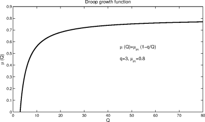
A note on the units: it is equally valid to think of the cell quota as either an amount of substrate per cell (nmol cell−1, as in Table 6.1) or as an intracellular concentration (convert using volume per cell). Now, Droop empirically found the relationship between cell quota and specific growth rate to take the form:
This is the Droop model or Droop equation. The subsistence quota, q, is the minimum quota necessary to sustain life. Figure 6.1 depicts the function µ(Q).
We still need to determine an expression for the cell quota, Q = Q(t). In general,
Where u is the specific rate of substrate uptake, and Φ is the rate of substrate depletion inside the cells. Assume the cell quota is at a steady-state. Since Q is unchanging, we have that the specific growth rate is constant, and the relation in equation (6.4), which states that medium substrate depletion is converted to (net) growth at a constant rate, holds, giving:
The conservation of substrate implies that
which is equivalent to
This follows from the chain rule,
and from equation (6.6). Finally, from the steady-state assumption for Q, we have
As to the form of the uptake term, u, Droop found a simple saturating function to describe the data well:
This completes the derivation of the basic cell quota model, which we restate in full:
The above model shall be supplemented with appropriate nonnegative initial conditions for all the variables and the additional requirement that Q(0) > q. Note that as long as Q(0) ≥ q, then Q(t) ≥ q.
There are several straightforward modifications to the basic framework that we may consider. The most obvious follows from the reality that the cell quota must have some upper limit, giving the common modification:
where qm is the maximum cell quota. In this case, the rate of uptake decreases linearly with cell quota. Alternatives include the addition of a Michaelis-Menton (Hill) term.
Growth rate subject to two potentially limiting nutrients may be modeled by the following cell quota based equation
6.3 From Droop cell-quota model to logistic equation
The main purpose of this section is to derive the logistic model via Droop equation. We consider a single species growing in a closed environment where there is a single most limiting nutrient. For convenience, we assume below that this species is an species of algae and the limiting nutrient is phosphorous P. Observe that the total amount of phosphorus PT in this closed growth environment remains constant.
If we let Px and Pf be the phosphorus in the algal cells and the free phosphorus respectively, then PT = Px + Pf. Let x = x(t) be the algal cell density and Q = Q(t) be the algae’s cell phosphorus quota. Then Px = Qx. Hence
In the following, we let q be the algae’s minimal cell quota of P, µm be the species’ maximal growth rate, D be its natural death rate. By (6.5), we have the following equation for the species growth:
The free phosphorus changes according to
The first term describes the loss of phosphorous due to the uptake by x cells which may be simply approximated by a mass action process. The second term assumes that the dead algal cells immediately release their phosphorous back to the growth environment.
We still need an equation governing the dynamics of Q, the species’ cell quota for P. However, this equation can be derived from the nutrient conservation equation (6.19). We have
This results in the following simple equation
We assume that Q(0) ≥ q and PT > x(0)Q(0). Mathematically, this ensures that Q(t) ≥ q for all t > 0.
Since the cell metabolic process operates at a much faster pace than the growth of total biomass of a species, the quasi-steady-state argument allows us to approximate Q(t) by the solution of
which takes the form of
This together with (6.19) yields
Substituting (6.26) into (6.25) yields
Substituting the above into (6.20) yields
The above equation can be rewritten as
We can further rewrite the above equation as
Or equivalently,
It clearly takes the form of the classical logistic model
with
and
From Eq. (6.34), we see that r and K are not independent. Indeed, they are linearly dependent. It is easy to observe that both r and K are increasing functions of α and decreasing function of D. This makes good biological sense. It should be pointed out here that we did not assume the population suffers from a crowding effect explicitly. However, this crowding effect is implicitly provided by the fact that the total nutrient in the system (here P) is fixed, and individuals have to compete for this resource. Observe that the expression of K is different from the intuitive carrying capacity of the form PT/q. The expression of K says that while in theory the environment may sustain a maximum of PT/q cells, the actual upper limit for the algae biomass can attain is K = (µm − D)PT /(qµm) − Dα−1, which is less than PT/q. The reason that the intuitive carrying capacity PT/q cannot be reached in practice is that the death process in a population keeps the population below its potential maximum. However, the equation (6.34) says clearly that a population with a relatively low death rate will likely amass more biomass than a population with a relatively high death rate.
Droop equation based population models are capable of generating rich and often intriguing dynamics that realistically match those observed in field and lab experiments ([27, 28], [41]).
6.4 Cell-quota models for prostate cancer hormone treatment
In the following, we present two cell-quota based models for prostate cancer hormone treatment due to Portz, Kuang and Nagy [33]. Their models aim to produce solutions match the data of clinical trials. With a data validated model, we can hope to gain a greater understanding of the processes at work in prostate cancer and androgen suppression therapy. Moreover, a model capable of predicting the course of an individual case of prostate cancer would be useful in developing a treatment schedule in a clinical setting. Their models are based on the works of Jackson et al.[18] and Ideta et al.[17]. These earlier models include an androgen-dependent (AD) cell population and an androgen independent (AI) cell population with mutation from the AD population to the AI population at a rate based on the androgen concentration. The material of this section is adapted from the content of Portz, Kuang and Nagy [33].
6.4.1 Preliminary model
In an initial model formulated by Portz, Kuang and Nagy [33], the growth rate of the AD cell population is given by Droop’s cell quota model. The cell quota model introduces a new variable, Q(t), which is the cell quota for androgen. The AD and AI cell populations are modeled by
The proliferation rate of the AD cell population is zero when Q(t) is at the minimum cell quota q. As Q(t) increases, the growth rate approaches its maximum, µm. The apoptosis rate of the AD cell population and the net growth rate of the AI population excluding mutation are assumed to be constant.
This model includes mutation between both cell populations. This change is made under the hypothesis that androgen dependence can be regained by AI cells in an androgen-rich environment with some sort of switching behavior. The switching rates are given by hill equations,
The AD to AI mutation rate, m1(Q), is low for normal and high androgen levels and high for low androgen levels. In contrast, the AI to AD mutation rate, m2(Q), is high for normal and high androgen levels and low for low androgen levels.
The cell quota for androgen within the AD cells is modeled by
Androgen within the cells is used for growth up to the minimum cell quota at a rate µm and is also assumed to degrade at a constant rate b.
The serum PSA concentration, P(t), is modeled as a linear function of the two cancer cell populations:
6.4.2 Final model
In the final model, Portz, Kuang and Nagy use the cell quota model for both the AD and AI cell populations [33]:
Both cell populations have the same maximum proliferation rate µm. To give the AI cells greater capacity for proliferation in low androgen environments compared to AD cells, they select a lower minimum cell quota for the AI cells, q2 < q1.
The relevance of the cell quota model follows from the nature of androgen’s action and how its signal is transduced. The AR is intracellular, so only intracellular androgen can be sensed, and proliferation depends on AR:androgen binding. Hence androgen is clearly a resource. For the AI cells, androgen receptors are typically either activated in an androgen-independent way, are amplified, or are otherwise activated by mutated regulators [22]. In any of these cases, the androgen receptor is still active and some AR:androgen response remains. However, far less androgen is required to achieve the same level of proliferation, which the Droop formalism captures very nicely with the constraint q2 < q1.
The cell quotas for androgen are modeled by the same equation as the preliminary model,
However, there are now two cell quota variables, Q1(t) for the AD population and Q2(t) for the AI population.
The switching rates between the AD and AI cell populations take the same form as in the preliminary model,
With this final model, a new model for the serum PSA concentration is introduced:
It is assumed that PSA is produced by both AD and AI cells at a baseline rate σ0 plus an additional androgen-dependent rate. Experimental evidence supports the assumption that PSA production is dependent on androgen levels [15]. Hill functions are used for the androgen-dependent rate so that it increases with the cell quota toward a maximum rate σi. The androgen-dependent rate is split into two terms, one for each cell population, because the two populations respond differently to androgen. It is also assumed that PSA is cleared from the blood at a constant rate δ.
6.4.3 Simulation
In a clinical study [1], seven men with stage C and stage D prostate cancer were treated with intermittent androgen suppression therapy. Androgen withdrawal was maintained for 6 or more months and then interrupted for 2 to 11 months. Serum androgen and PSA concentrations were measured on a monthly basis. When serum PSA concentrations exceeded a threshold of about 20 ng/mL, androgen withdrawal was resumed. This treatment cycle was continued over periods of 21 to 47 months. Portz et al. used the androgen and PSA time series data from the seven cases to simulate and fit the models [33]. Using clinical data from an intermittent androgen suppression trial provides a better assessment of the dynamics of prostate cancer as responses to both the initiation and withdrawal of treatment can be observed as opposed to continuous androgen suppression where only a single on-treatment period is observed.
The serum androgen data from the clinical cases is used directly as A(t) for fitting rather than modeling the androgen concentration. However, the coarse androgen data must be interpolated before it can be used as an input to the numerical simulations. Using linear interpolation results in the peaks of the PSA concentrations being significantly delayed. These delays are caused by the slow linear decline in androgen concentration between off-treatment and on-treatment periods in the simulations when the actual androgen concentrations drop very quickly. To obtain more accurate results, an exponential fit is used between the last off-treatment data points and the first on-treatment data points,
where ti is the time of off-treatment data point, tf is the time of the on-treatment data point, and γ is the serum androgen clearance rate. The remaining segments of the androgen data are interpolated using piecewise cubic hermite splines to give smoother responses in the simulations.
The parameters of the models are initially fit by hand to provide good qualitative fits with the clinical PSA data. Once a reasonably close fit has been obtained, a simplex search method is used to minimize the mean square error between the clinical PSA data and the simulated PSA concentrations. This parameter fitting is performed for each of the seven cases on all three models.
The simulation result for the final model for subject 1 described in [1] is shown in Figure 6.2. This model is better at fitting the clinical PSA data than either the preliminary model or the model of Ideta et al. [33].
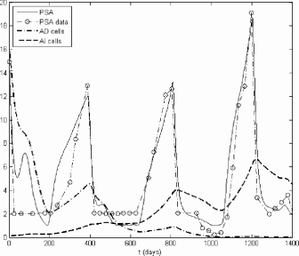
Table 6.2 shows the mean squared error between the simulated PSA levels and the clinical PSA levels for each case and model as reported in [33]. The table also presents a comparison based on the Schwarz Bayesian Criterion, which includes an adjustment for the number of free parameters. The results clearly confirm that the final model produces the best fits out of the three.
Comparison of model fits, including mean squared error (MSE) and Schwarz Bayesian Criterion (SBC). Lower values indicate better fits for both MSE and SBC.
MSE |
SBC |
|||||
|---|---|---|---|---|---|---|
Case |
Ideta |
Prelim. |
Final |
Ideta |
Prelim. |
Final |
1 |
21.21 |
30.61 |
2.960 |
145 |
145 |
68.0 |
2 |
25.65 |
96.05 |
2.790 |
85.9 |
112 |
41.5 |
3 |
216.6 |
238.2 |
46.42 |
185 |
188 |
139 |
4 |
12.26 |
13.60 |
3.924 |
93.5 |
96.4 |
61.6 |
5 |
358.1 |
497.3 |
41.81 |
101 |
105 |
70.7 |
6 |
44.59 |
41.91 |
0.3985 |
96.9 |
95.7 |
2.57 |
7 |
6.655 |
6.588 |
3.710 |
67.7 |
67.5 |
53.7 |
Overall |
81.40 |
106.3 |
13.46 |
806 |
853 |
491 |
6.4.4 Predictions
The result of running the final model for another treatment cycle beyond the clinical data for subject 1 is shown in Figure 6.3 and the results for the other subjects can be found in [33]. It is known that the patients in cases 1, 2, 3, and 5 had stage C cancer, while the patients in cases 4, 6, and 7 had stage D (metastatic) cancer [1]. The final model can be used to predict uncontrolled growth in the AI population for the stage D cases even though the PSA concentrations do respond to the final on-treatment period in cases 6 and 7. The model also predicts a poor response to another treatment cycle for the patient in case 3, who had already undergone two long treatment cycles.
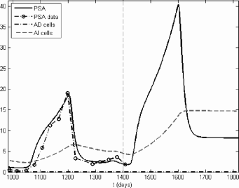
Prediction of the final model, case 1. The dashed vertical line separates the clinical fit and the prediction. The PSA concentration and AI population increase significantly with another off-treatment period. However, the subsequent on-treatment period remains effective in stopping further growth.
In [13], Everett, Packer and Kuang extended the above final model in two ways and tested their models predictive accuracy, using only a subset of the data to find parameter values. The results are compared with the piecewise linear model of Hirata et al. [22] which does not use testosterone as an input (see Section 5.11). Based on a small set of data from seven patients contained in [1], their results showed that the piecewise linear model actually produced slightly more accurate results while the two more biologically plausible predictive methods are comparable. However, this comparison did not penalize the excessive number of parameters (since each on and off treatment requires a new set of parameter values) used in the piecewise linear model of Hirata et al. [22]. Nevertheless, it suggests that a simple piecewise linear model may still be useful for a predictive use despite its simplicity and lack of close biological connections.
6.5 Other cell-quota models for prostate cancer hormone treatment
In Section 6.4, we described two cell-quota models for prostate cancer hormone treatment due to Portz et al. [33]. They modeled androgen-limited growth in prostate cancer using a Droop model, with androgen-dependent and independent cell lines characterized by different subsistence quotas (q), and modeled intermittent androgen suppression therapy. Excellent agreement between the model and clinical data was achieved with this approach. We develop below several similar models for competition between AI and AD cells.
6.5.1 Basic model
We consider a model very similar to that of Portz et al. [33]. We have two strains of cell, X1(t) and X2(t), with differing sensitivities to androgen. We let these variables represent the absolute numbers of cells, rather than cells l−1 as above (which follows Droop’s original derivation). The cell-quota model above can be reformulated using absolute cell count and substrate amount, and it remains essentially identical, although care must be taken to appropriately convert substrate amount to concentration, based on medium volume. For parametrization, we take cell quota to be in units of concentration (nM), by converting from nmol cell−1 to nmol l−1 (nM).
The cell quota for this model is intracellular androgen concentration (presumably complexed to its receptor, with units nM), still represented by Q. The basic cell quota model for androgen-mediated growth is:
The mutation rates between strains are given by m1 and m2, and, unlike in Ideta’s or Portz et al.’s models, are constants, and background cell death occurs at rates d1 and d2. We have the cell quotas governed by:
Androgen uptake is saturable according to the parameters, and cell quota is limited by the second Hill function in the uptake term. Finally, androgens positively regulate the expression of PSA by prostate epithelium, so rather than take the serum PSA level as a simple linear conversion from cell mass as done by Ideta et al. [17], we model PSA dynamic quantity with the same governing equation as done by Portz et al. [33] which is identical to (6.39):
where σ0 is the baseline level of PSA production by all cells, and androgen induces each strain to increase production according to their respective Hill functions.
6.5.2 Long-term competition in the basic model
Portz et al. [33] modeled increased sensitivity to androgens by AI cells, X2(t), by making the subsistence quota for such cells smaller than that for AD cells, namely q2 > q1. While apparently reasonable, such a choice results in the cell quota for AI cells being smaller than for AD cells (a growth advantage does still exist for such AI cells). We argue that, under the basic model, modifying the uptake parameters and may better represent increased sensitivity to androgen via such AR upregulation or other common mechanisms. And indeed, making either or results in a greater Q2 and a selective advantage for AI cells that stems from their larger cell quota.
Before examining intermittent androgen deprivation, we briefly re-address the evolutionary question posed in Section 5.4: how do serum androgen levels affect the early evolution of prostate cancers? The model of Eikenberry et al. [8] suggested that low systemic androgen may induce selective pressure for highly androgen-sensitive strains, which may have higher malignant potential or give rise to cancers poorly responsive to treatment. We apply the basic model just presented to this problem by letting . We also make growth space-limited as follows:
where K is the carrying capacity of the normal prostate. This change also necessarily affects the cell quota loss term, −µiQi. We simulate the model starting with AD cells at their approximate equilibrium point with no AI cells present, and we set the serum androgen level, A, to a constant.
Figure 6.4 shows the evolution of the two strains under different values for A. As in Section 5.4, this model, independently derived from quite different principles, suggests that low systemic androgen selects for cell strains with reduced androgen dependence. Again, more androgen-sensitive strains are also ultimately selected for in normal and high-androgen environments, but in such environments the selective pressure is weaker. The time from the start of the simulation until AI cells become a majority is plotted in Figure 6.5, and this time increases nearly linearly with serum androgen.
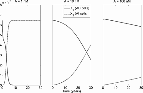
Competition between AD and AI cells in a prostate under the basic cell quota model with space-limited (logistic) growth. AI cells have greater uptake of androgen, with and . From left to right, A is fixed at 1 nM, 10 nM, and 100 nM. Parameter values are µm = 0.035, d1 = d2 = 0.01, q1 = q2 = 0.3, m1 = m2 = 10−5, b = 0.09, , , , um = 0.275, σ0 = 10−10, σ1 = σ2 = 5 × 10⁻¹⁰, m = 2, ρ1 = ρ2 = 1.2, δ = 0.2.
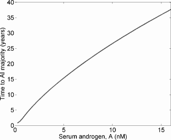
Under the same model as in Figure 6.4, the time until AI cells become a majority as a function of serum androgen, A.
Reasonable parameter values for the model, based on the chemical kinetics model of Section 5.4.2, Ideta et al. [17], and Portz et al. [33], are reported in the caption of Figure 6.4.
6.5.3 Intermittent androgen deprivation
Akakura et al. [1] used the following algorithm in a clinical study of intermittent androgen deprivation: androgen withdrawal was initiated pharmacologically. Following 6 months of PSA in the normal range, treatment was stopped; it was resumed once serum PSA exceeded 20 ng/ml. Portz et al. [33] achieved an excellent match between his model and the clinical data in this study. Figure 6.6 shows the results of intermittent androgen suppression with A set at either 0.5 nM or 0.1 nM during therapy and at 15 nM off therapy. Treatment is given for a fixed period of 180, 90, or 30 days, and resumed when PSA > 20 ng/ml.
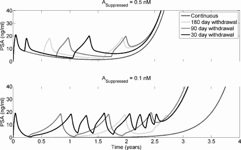
Intermittent androgen deprivation therapy under the Droop model presented in Section 6.5.1. Parameter values are as in Figure 6.4, except µm = 0.025, m1 = m2 = 10−6, and . Note that the advantage to continuous depravation in the lower panel disappears if KA2 is made sufficiently small.
From Figure 6.6, it can be seen that all suppression periods generate essentially identical results. When androgen deprivation is severe, continuous deprivation may be superior to intermittent therapy. However, this result depends entirely on the androgen sensitivity of the AI line. If the AI line is capable of responding to even very low androgen levels, i.e. is made sufficiently small, this advantage disappears.
The Droop model predicts then, that even very brief periods of androgen deprivation are likely to suppress tumor growth as well as other schedules. Since clinically maximal androgen blockade has not proven superior to standard therapy, it is likely that brief intermittent therapy is nearly as good as continuous therapy.
6.5.4 Cell quota with chemical kinetics
We now propose a somewhat more complex model that takes the intracellular chemical kinetics of androgens into account. For simplicity, we consider only testosterone (T) and disregard DHT for the moment. The cell quota, Q, is now taken to be the intracellular T:AR complex concentration (nM). From first principles, we have that T is a steroid hormone that freely crosses cells membranes, and we have a system for intracellular free testosterone, Ti, free AR, Ri, and T:AR complex Qi, all in nM units:
Note that we disregard production and loss of both free and complexed AR. In the chemical kinetics model of Section 5.4.2 we did consider these behaviors, but the model was such that the total AR concentration within the cell remains constant. Our simplification here is therefore a “shortcut” to the same essential behavior.
The parameter Ai is the surface area of vasculature associated with strain i and can be calculated as:
where α is a constant with units m2 cell−1. The permeability coefficient of testosterone is P (m hr−1), and γ is a constant giving the volume in L per cell. The other kinetic parameters are as in Section 5.4.2.
This model allows us to more realistically model upregulation of the AR as a mode of androgen independence. We leave such investigation to the student. We also leave it as an exercise to extend the model to consider conversion of T to DHT by 5α-reductase, and the appropriate modification of the cell quota.
6.6 Stoichiometry and competition in cancer
Tumors compete for resources with their hosts. As we have discussed at various points in this and other chapters, healthy cells and multiple strains of cancer cell must compete for space, oxygen, glucose, growth factors, and, as we discuss here, elemental nutrients. A striking demonstration of a tumor’s effect on the host physiology is cancer cachexia, a complex wasting syndrome characterized by weight loss, anorexia, and neurohormonal abnormalities. A combination of tumor and host factors cause progressive breakdown of skeletal muscle, fat, and bone that is not reversible by nutritional supplementation; resting energy expenditure is often increased and there is increased glucose production and catabolism [43].
Ecological stoichiometry is an increasingly important field which studies the balance of elements in ecological systems. In particular, organisms vary greatly in their relative nitrogen (N), carbon (C), and phosphorus (P) content. Phosphorus is a key element in ecological systems, and multiple lines of evidence point to it being a key resource that healthy and cancerous cells may compete for. Phosphorus is an essential component of DNA and RNA, and the majority (about 80%) of RNA is incorporated into ribosomes, vast molecular factories that translate mRNAs into proteins. The proteins produced by ribosomes are essential for rapid cell growth and proliferation, and multiple studies indicate that ribosome synthesis is essential to rapid cancer cell proliferation [23]. Hence, the importance of phosphorus. Note also that nitrogen is an essential component of both the nitrogenous bases that make up RNA and DNA, and of the amino acids that compose proteins. Glucose, a six-carbon chain, provides energy. Thus, the three elements studied in ecological ecology are essential factors in the tumor-host ecology as well.
The growth rate hypothesis posits that organisms with a rapid growth rate require a high P content in biomass, due to the requirement for high-P content ribosomes [10]. Thus, rapid growth as an evolutionary strategy has the cost of increased dependence on environmental or dietary phosphorus. Translating this to tumor biology, the hypothesis predicts that rapidly growing tumors should have a high P content, but there is an evolutionary cost in P-limited environments.
6.6.1 KNE model
Kuang, Nagy and Elser have recently applied ideas from ecological stoichiometry to tumor growth, and have proposed a mathematical model for phosphate-limited growth in human cancer [23]. The model considers a cancer of some organ which, for concreteness, we take it to be the lung. Let x represent the mass of healthy cells in the organ, yi represents cancerous cells of strain i, and z is the total tumor microvessel mass. We assume the organ has an overall mass of KH, and the tumor’s maximum size is KT.
Phosphate-limited growth. Now, considering phosphorus mass, P, we assume the total phosphorus in the organ remains constant. We assume n represents the average amount (grams) of phosphorus per kg of healthy tissue; likewise mi is phosphorus mass per kg of cancerous tissue of strain i. That is, these are units of concentration. Thus, we have:
where Pe is mass of extracellular P within the organ. The extracellular volume is given by f × KH, where f is the fraction of organ mass that is extracellular (about 1/3), and KH is the organ mass. Therefore, extracellular concentration is simply:
Now, we assume that if the extracellular P concentration, [Pe], falls below the mean for healthy cells, n, then the maximal proliferation rate, a, is impaired. That is, cells proliferate at rate a when sufficient P is present ([Pe] ≥ n), and at rate
when [Pe] < n. Malignant cells similarly depend on [Pe] and mi and have maximum growth rate bi.
Vasculature-limited growth. Tumor growth requires a sufficient vasculature. We define L as follows:
Here, α is the mass of cancer cells that can just barely be supported by a unit of blood vessels, and g measures the sensitivity of tumor cells to hypoxia. If L ≥ 1, then proliferation is unimpaired, but if L < 1, then the growth rate is modified by the factor L. We also assume that cancer cells generate some signal that recruits immature endothelial cells to form blood vessels at rate c. We can incorporate a delay into the model by assuming it takes τ time units for vessels to form in response to this signal.
Space-limited growth. We have growth limited by organ size. Healthy cells grow to a carrying capacity of KH, with all cells competing for this space. The tumor mass grows to a carrying capacity of KT. Healthy cells do not affect the maximum tumor size, from the assumption that cancer cells better compete for space. We also assume that healthy, malignant, and endothelial cells undergo death at per-capita rates dx, di, and dz, respectively.
Model. The above considerations give the model for two strains of cancer cells, i = 1, 2:
Note that we have added the coefficient βi to represent the relative efficiency of P uptake by cancer cells. Finally, the model may be modified to consider a changing phosphate load in the organ. We assume a constant influx of P at rate r, representing dietary intake. When cells die, they liberate P; a small amount of the liberated P will not be recycled, but will be lost to the circulation. We let γ represent the fraction lost, and have:
6.6.2 Predictions
Kuang et al. [23] estimated the phosphorus content of the lung to be roughly 150 g. We also assume that growth rate for different cell lines scales linearly with cellular phosphate concentration (i.e., a 10% increase in P increases the specific growth rate by 10%). From numerical simulation of the model with fixed P (results are essentially the same using equation (6.62) for P dynamics), it is clear that when total organ phosphorus is below some threshold, rapidly growing cancer strains may dominate early in time, but slower growing lines dominate with large time, and the faster growers are driven to extinction. If organ phosphorus is sufficiently plentiful that space becomes limiting before phosphorus, then rapid growers dominate. However, in this case there is coexistence of the slow and rapid growers. These results are summarized graphically in Figures 6.7 and 6.8.
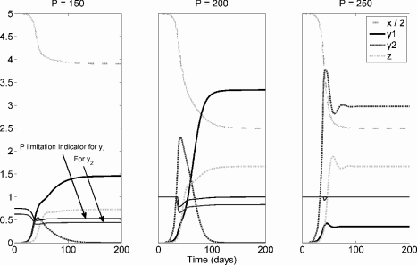
KNE model for phosphate-limited tumor growth under different values of total organ phosphorus, P. Parameter values are a = 0.3; n = 10, b1 = 0.6, m1 = 20, b2 = 0.72, m2 = 24, dx = d1 = d2 = 0.1, dz = 0.2, c = 0.1, α = 0.05, g = 100, KT = 5, and KH = 10.
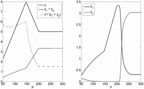
The left panel gives long-term total tumor mass (y1 + y2), healthy cell mass (x), and the ratio of healthy to cancerous tissue (x/(y1+y2)), for different values of total organ phosphorus under the KNE model. The right panel gives the long-term population size of slowly (y1) and rapidly growing (y2) tumor cell strains. See Figure 6.7 for parameter values.
This gives the counterintuitive prediction that slow-growing cell lines can dominate the tumor over time and continually threaten faster-growing lines with extinction. Kuang et al. suggested that this may provide the evolutionary impetus for aggressive growers to spread metastatically to distant sites, replete with phosphorus.
On the surface, phosphate-limited tumor growth suggests limiting phosphate by dietary restriction or with pharmacologic phosphate binders as a clinical treatment strategy. However, limiting P also harms the healthy tissue. From Figure 6.8, it can be seen that the ratio of healthy to tumor tissue is maximized when P is about 150 g (at least for this parameter set). Decreasing P reduces both tumor and healthy cell mass, but is relatively more deleterious to healthy cells. Increasing P fuels tumor growth to the detriment of healthy tissue, and there is a region where tumor mass is quite sensitive to increases in P.
6.7 Mathematical analysis of a simplified KNE model
For realistic parameter values and initial conditions, the ultimate outcome of the KNE model (6.61) is that solutions tend to a positive steady state where phosphorus limits both healthy and tumor cell growth. Unfortunately, it is difficult to find an analytic expression of this positive steady state and even more daunting to determine its stability properties. However, near this steady state, tumor growth shall be minimally limited by its blood vessel infrastructure since it has enough time for the infrastructure to be put in place. This presents a realistic simplification of the KNE model. Therefore, in this section we will assume that
(A1): The construction of blood vessels is not limited by phosphorus supply.
With (A1), the KNE model (6.61) becomes the following simplified model:
Additional support for the validity of assumption (A1) comes from the fact that the difference between ultimate sizes of tumors described by the KNE model (6.61) and the simplified KNE model (6.63) are negligible.
In the following, we will study the stability of the positive steady state E* of model (6.63). Our analysis is simplified by the following observation from simulation results: at this steady state E*, and L > 1 (see Figure 6.9). Hence we assume further that
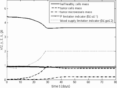
A solution for model (4.1) with a = 3, m = 20, n = 10, Kh = 10, Kt = 3, f = 0.6667, P = 150, α = 0.05, b = 6, τ = 7, c = 0.05, dx = dy = 1, dz = 0.2, g = 100 and (x(0), y(0), z(0)) = (9, 0.01, 0.001). Here we assume no treatment blocking phosphorus uptake by tumor cells (β = 1) and the construction of blood vessel is NOT phosphorus limited. Notice that and L > 1 at E* for model (6.63).
(A2): For model (6.63), and L > 1 at E*.
Clearly (A2) implies that . With this additional assumption, model (6.63) is further reduced to
This reduced model has a unique positive steady state E* = (x*, y*, z*):
where
and
Notice that y* = 0 if and only if
This yields a threshold value for β, which we denote by β*,
In order to study stability aspects of the steady state E* of model (6.64), appropriate methods from the theory of delay differential equations are needed. The recent textbook on this subject by Smith [39] is a timely and easy to follow reference. However, to obtain some quick result, we can apply the following lemma, the proof of which follows directly from that of Theorem 6.5.2 (page 227) in Kuang, 1993 [20].
Assume that the parameters in the following system are positive, and x* > 0, y* > 0, z* > 0:
If there are positive constants c1, c2 such that
- (1): dz > c/c2,
- (2): B2/c2 > B3 + B1/c1,
- (3): A1/c1 > A1 + A2/c2
then the steady state E* = (x*, y*, z*) is globally asymptotically stable.
Near the steady state E*, model (6.63) can be rewritten in the form of system (6.68) with
and
For a = 3, m = 20, n = 10, Kh = 10, f = 0.6667, P = 150, b = 6, dx = 1, dy = 1, β = 1, we can chose c1 = 0.5 and c2 = 0.2 to satisfy conditions 1) through 3) in Lemma 6.1. In other words, we have shown that for this set of parameters, the positive steady state E* of model (6.64) is locally asymptotically stable. However, simulation suggests that it is actually globally asymptotically stable. So, this mathematical question remains open.
As we increase P in model (6.64), the condition may be violated, and the positive steady state may become the positive solution of
where Bi, i = 1, 2, 3 are given by equation (6.70). In this case, we have
Using Lemma 6.1, we can also show that this steady state is locally asymptotically stable.
A sufficiently large increase in P will lead to a scenario in which .
For example, when a = 3, m = 20, n = 10, Kh = 10, f = 0.6667, P = 150, b = 6, dx = 1, dy = 1, β = 1, we need P > 257.34. In such a case, the positive steady state is simply E* = (Kh − Kt, dzKt/(c + dz), cKt/(c + dz)), which again by Lemma 6.1, is locally asymptotically stable.
We summarize the above statements into the following theorem.
Assume that in model (6.64) there is a unique positive steady state E* = (x*, y*, z*). Assume further that there are positive constants c1, c2 such that
- (1): dz > c/c2,
- (2): B2/c2 > B3 + B1/c1,
- (3): A1/c1 > A1 + A2/c2
where A1, A2, B1, B2, B3 are given by equations (6.69) and (6.70). Then the steady state E* = (x*, y*, z*) is locally asymptotically stable.
In an interesting special case when ma = nb, dx = dy, β = 1, we have
where
This expression of tumor steady state size shows that P plays a prominent role in determining its value. We observe that the tumor dies out if one can increase the tumor’s death rate or the tumor’s P requirement m, or lower the tumor’s proliferation rate to certain threshold levels.
6.8 Exercises
Exercise 6.1: Explicitly derive a version of the Droop model that considers cell mass in terms of absolute cell count (units cells) rather than cells l−1. Confirm that the cell quota Q has the same units as before.
Exercise 6.2: The basic cell quota model of biomass growth in a batch culture (a closed system in which cells are grown in a fixed volume of nutrient culture medium under specific environmental conditions) takes the form of
with positive initial values. All parameters are assumed to be positive constants. Show that
- i): Explain the model formulation. (Hint: s(0) = s(t) +x(t)Q(t))
- ii): If Q(0) ≥ q, then Q(t) ≥ q, ;
- iii): The solution tends to a nonnegative steady state that is dependent on its initial condition.
Exercise 6.3: Use IVIATLAB ® to simulate model system (6.74)-(6.76) with your own positive parameter values and appropriate positive initial value. Print out several representative simulation figures.
Exercise 6.4: Chronic myeloid leukemia (CIVIL) is a cancer of the white blood cells. CIVIL can be molecularly diagnosed by detecting the presence of the Philadelphia (Ph) chromosome and the fusion oncogene BCR-ABL. This oncogene is the result of translocation of the BCR, or breakpoint cluster, gene located on chromosome 22 and the ABL, or Ableson leukemia virus, gene located on chromosome 9. The growth rate of the BCR-ABL dependent and independent cell populations are modeled using the Droop’s cell quota model, where Q(t) represents the cell quota for BCR-ABL. The BCR-ABL dependent, BCR-ABL independent, and normal populations are modeled respectively by the following [14]:
We assume that the proliferation rates, , i = 1, 2, of both BCR-ABL dependent and independent populations are BCR-ABL cell quota dependent while the proliferation rate, , for the normal population is density dependent. We assume q1 > q2,
All parameters are positive constants. Show that the solutions of (6.77)-(6.80) stay in the region {(x1, x2, x3, Q) : x1 ≥ 0, x2 ≥ 0, , provided that x1(0) ≥ 0, x2(0) ≥ 0, x3(0) ≥ 0, qm1 ≥ Q(0) ≥ q1.
Exercise 6.5: Show that the system (6.77)-(6.80) has two possible boundary equilibria: E0 = (0, 0, 0, Q1), . Can it have any interior equilibrium? Find the local stability conditions for the boundary equilibria. Show that the system (6.77)–(6.80) has no positive periodic solutions.
Exercise 6.6: Consider the following case of phosphorus-limited growth in some species. Let Pt = total environmental P, which remains constant. Let Pf be the free P, and we have the total intracellular phosphorus as Px = Qx. Hence
Assume that P uptake increases linearly with free phosphorus Pf and the difference of the maximum cell quota and the current cell quota of the phosphorus, giving:
and use the following equation for species growth,
which is simply the Droop equation for growth supplemented by a constant death rate.
Using a quasi-steady-state argument for Q, show that when QM >> 1, this model can be approximated by the classical logistic growth model of the form
where
Show that both r and K are increasing functions of α and decreasing function of d.
- Give a biological interpretation of these results.
- (a) Consider the simplified case where d = 0. What do r and K reduce to, and give a biological interpretation. What is the significance of the ratio Pt/q?
- (b) How do you expect a species with high turnover (i.e., high specific growth rate and death rate) would compete with one with low turnover?
- (c) How does increasing µm affect r and K if phosphorus uptake (α) is not increased?
- (d) How does increasing α affect r and K?
Exercise 6.7: Derive the equation (6.67) for the expression of β* and the equation (6.72) for the expression of y*.
Exercise 6.8: Reproduce Figure 6.9.
Exercise 6.9: Apply the Theorem 6.5.2 (page 227) in Kuang, 1993 [20] to prove Lemma 6.1.
Exercise 6.10: The following simple delay differential equation model was introduced in Everett et al. [12] to describes ovarian tumor growth and tumor induced angiogenesis, subject to on and off anti-angiogenesis treatment. Let y represent the vascularized tumor volume and Q represent the intracellular concentration of necessary nutrients provided by angiogenesis, or the cell quota of some limiting nutrient from angiogenesis. The model takes the following form:
The above model assumes that it takes τ units of time for the vascular endothelial cells to respond to the angiogenic signal and mature to fully functional vessels and that the nutrient uptake rate is proportional to the nutrient concentration in the interstitial fluid, which in turn is proportional to the blood vessel density τ time units in the past. The delay arises because the tumor is assumed to grow into regions that are unvascularized, and it takes τ units of time for them to vascularize. Parameter α represents both uptake rate of the nutrients in the interstitial fluid and resulting nutrient concentration per tumor unit.
Show that the solutions of the system (6.86) with the initial conditions Qm > Q(t) > q and y(t) > 0 for t ∈ [−τ, 0] will remain in that region for all t > 0, where If µm ≤ d, then limt→∞ y(t) = 0.
Exercise 6.11: The uptake of nutrients is usually on a faster time scale than the population growth dynamics. If we apply a quasi-steady state argument on the cell quota equation in system (6.86) by allowing Qʹ = 0, we have
and so
Show that
Show that if , then the solutions of the limiting system (6.87) tend to y = 0.
Exercise 6.12: Motivated by the off-treatment tumor growth data in [19], Everett et al. [12] looked for the existence of a dominating exponential solution. Let y(t) = y0eλt. Then
- Show that if α(µm − d) > µmqd, then there exists a unique real eigenvalue, 0 < λ1 < µm − d, that satisfies (6.88).
- Show that (y1(t), Q*) is a solution to the limiting system (6.87) where
Exercise 6.13: Show that if α(µm − d) > µmqd and , then λ1 ≥ sup{Re(λ) : λ is any solution of (6.88)}.
This result provides a sufficient condition that ensures λ1 as the dominant eigenvalue, i.e. when the solution can be approximated by (6.89) for some y0 > 0. Also, note that since is a solution to the system, we know that y(t) is not bounded above.
Exercise 6.14: Show that if , then the solution of equation (6.88) is unstable.
Exercise 6.15: During an anti-VEGF treatment, the blood vessel growth will be impaired due to the inhibition of VEGF, but existing vasculature is likely not to be affected by the treatment. In that case nutrient delivery remains constant due to the static vasculature. One may assume that blood vessel sprouts that began forming within τ time units before the onset of treatment will not be fully formed and functional. Let t0 represent the time of treatment onset and ȳ = y(t0 − τ). Then nutrient delivery is dependent upon ȳ, and the delay differential equation model (6.86) becomes an ordinary differential equation model:
- Show that the solutions of the system (6.90) are bounded away from zero.
- Show that the solutions to the system (6.90) are bounded from above.
- The only positive equilibrium point E*, when exists, is globally asymptotically stable with respect to positive initial value (y0, Q0) such that QM > Q(0) =Q0 > q and y0 = y(0) > 0 where
Exercise 6.16: Fit model system (6.86) to the on and off treatment preclinical data sets from Mesiano et al. [19] with τ = 10, µm = 0.41, d = 0.28, q = 0.0064, α = 0.050, p = 0.17, Q0 = 0.014. You can use some computer program such as Plot Digitizer to approximate the on and off treatment data from Mesiano et al. [19].
6.9 Projects
The KNE model described in this chapter shall be viewed as only an initial attempt to understand the growth dynamics of a single vascularized solid tumor growing within the confines of an organ, such as a primary lung or breast tumor. In this section, we point out one of its main limitations and some opportunities for alternative model formulations and some natural extensions. In addition, we briefly mention a few other biomedical examples of nutrient-limited growth or resource competition that may be of interest to the readers.
6.9.1 Beyond the KNE model
6.9.1.1 Phosphate homeostasis
The most significant limitation of the KNE model is that it makes phosphate regulated at the level of total organ phosphate, rather than extracellular serum phosphate. In reality, serum phosphate concentration is held within a narrow range by endocrine regulation, about 3–4.5 mg/l. Because bone mineral is made of calcium-phosphate complexes in the form of hydroxyapatite, Ca5(PO4)3(OH), phosphate homeostasis is intimately linked to calcium homeostasis, and skeletal bone serves as a dynamic reservoir and buffer for both phosphate and calcium. Indeed, about 85% of the body’s phosphate is stored in the bone, and total body phosphate is at a dynamic steady state governed mainly by dietary intake (about 16 mg/kg/day), liberation and storage in the bone (about 3 mg/kg/day), and renal excretion (about 16 mg/kg/day) [3].
6.9.1.2 Intracellular phosphate: A Droop approach?
Extracellular phosphate levels are hormonally regulated to remain within a narrow range, and the intracellular concentration of ribosomal phosphate is clearly the relevant metric for determining cellular growth rate, suggesting that a Droop-like model may be well-suited to this problem. Indeed, our Droop model for androgen-limited growth discussed in Section 6.5.4 could be adapted.
6.9.1.3 Tumor lysis syndrome
Tumor lysis syndrome (TLS) is a complication of chemotherapy where large numbers of dying cancer cells release their intracellular contents into the systemic circulation, leading to high levels of phosphate, potassium, uric acid, and consequence hypocalcemia. These derangements can lead to life-threatening kidney failure and cardiac arrhythmias [16]. We can speculate that the phosphate liberated by chemotherapy, even if it does not lead to overt TLS, could fuel fast-growing cancer cell lines, causing a post-therapy tumor growth burst. Moreover, this abundant phosphate could give fast growers at least a transient selective advantage, possibly increasing the aggressiveness of a recurring tumor. Such an idea could be tested mathematically with a model that considers the positive contribution of cell death to serum phosphate concentration.
6.9.2 Iodine and thyroid cancer
In response to pituitary thyroid stimulating hormone (TSH), the thyroid gland produces thyroid hormone (TH), which modulates metabolic activity by nearly every cell of the body. Iodine is an essential component of the thyroid hormones, and iodine dietary intake clearly affects the incidence of thyroid cancer. Chronic iodine deficiency greatly increases the risk of benign thyroid goiters and nodules, which in turn are susceptible to malignant transformation. Thus, iodine deficiency is clearly associated with an increased cancer risk. The effect of excess iodine is less clear, but it too may increase cancer risk [30].
Iodine deficiency continues to affect a significant proportion of the globe, although iodization of salt has ameliorated the problem in much of the world. Introducing iodine to chronically iodine-deficient populations can also result in reactive hyperthyroidism, as thyroids adapted to low iodine levels are suddenly flush with the element.
6.9.3 Iron and microbes
Iron is an essential nutrient required by all pathogenic microorganisms as well as the hosts they infect. Unlike essentially all other nutrients, iron is not freely available to pathogens, and its transport and storage is tightly regulated by the host. Thus, iron can be viewed as the critical limiting element in pathogen growth [34].
Iron acts on several levels in infection. It is an essential cofactor in a number of metabolic pathways required for energy production and cellular replication. Iron is also essential to innate host immune responses, being required for energy production and the generation of nitric oxide and other reactive oxygen species (ROS) that play an essential role in destroying intracellular pathogens [5]. In a variety of microbial infections both iron overload and deficiency can increase morbidity and mortality [5]. Thus, competition between the host and pathogen for iron is essential in determining the course of disease.
Salmonella, for example, infect macrophages which destroy most bacteria within hours by iron dependent mechanisms (e.g. the respiratory burst). Surviving bacteria enter a cytostatic state of bacterial persistence, and iron load may be crucial to the switch to bacteria persistence. Epidemiologically, iron overload and deficiency increase both salmonella infection and disease virulence.
Intracellular pathogens compete with and/or exploit host iron trafficking mechanisms in a number of ways. For an exhaustive review of iron trafficking and metabolism in bacterial pathogens, see [34].
6.9.3.1 Salmonella infection
Salmonella primarily infects mononuclear macrophages, and intracellular survival in these cells is essential to in vivo virulence. When responding to a salmonella infection, macrophages execute two killing programs. The first is the respiratory burst, which primarily contributes to early killing. Inducible nitric oxide synthase (iNOS) is one of three key enzymes generating nitric oxide (NO). NO generation by iNOS is the second major pathway, and contributes to both early and late stage killing [44]. Both pathways are dependent upon iron, and NO may act synergistically with oxygen radicals generated by the respiratory burst.
This response leads to a pattern of infection where 99% of bacteria are killed within the first few hours of infection, while the survivors enter into a cytostatic state of bacterial persistence [44]. There is a delicate balance between pro-oxidant and antioxidant effects of NO in salmonella; this balance is largely mediated by iron, and iron load may be crucial to the switch to bacteria persistence. This is particularly relevant as 2–5% of infections can lead to asymptomatic chronic carrier states.
Epidemiologically, iron overload and deficiency both increase salmonella infection and disease virulence. Treatment with the intracellular iron chelator deferoxamine resulted in a 2–3 log increase in bacterial load, while extracel-lular iron chelation did not affect the disease [5].
An interesting area that could be investigated with modeling is understanding how iron load affects progression to a bacteriostatic state, and how dietary intervention or treatment with chelators could influence the chronic infection state.
6.9.3.2 Malaria
Malaria induces a cytokine mediated host response that induces iNOS and NO production. Malaria infection causes anaemia, but can increase iron concentration in the liver and spleen due to recycling of heme-bound iron stored in both infected and uninfected erythrocytes eliminated by macrophages. This inhomogeneous iron load may affect the course of disease, and salmonella co-infection with malaria may be an interesting and important area to study.
References
[1] Akakura K, Bruchovsky N, Goldenberg SL, Rennie PS, Buckley AR, Sullivan LD: Effects of intermittent androgen suppression on androgen-dependent tumors. Apoptosis and serum prostate-specific antigen. Cancer 1993, 71:2782– 2790.
[2] Berges RR, Vukanovic J, Epstein JI, CarMichel M, Cisek L, Johnson DE, Veltri RW, Walsh PC, Isaacs JT: Implication of cell kinetic changes during the progression of human prostatic cancer. Clin Cancer Res 1995, 1:473–480.
[3] Bergwitz C, Jüppner H: Regulation of phosphate homeostasis by PTH, vitamin D, and FGF23. Annu Rev Med 2010, 61:91–104.
[4] Bruchovsky N, Klotz L, Crook J, Goldenberg SL: Locally advanced prostate cancer-biochemical results from a prospective phase II study of intermittent androgen suppression for men with evidence of prostate-specific antigen recurrence after radiotherapy. Cancer 2007, 109:858–867.
[5] Collins HL: The role of iron in infections with intracellular bacteria. Immunol Lett 2003, 85:193–195.
[6] Droop MR: Vitamin B12 and marine ecology, IV: The kinetics of uptake, growth and inhibition in Monochrysis lutheri. J Mar Biol Assoc, UK 1968, 48:689–733.
[7] Droop MR: Some thoughts on nutrient limitation in algae. J Phycol 1973, 9:264–272.
[8] Eikenberry SE, Nagy JD, Kuang Y: The evolutionary impact of androgen levels on prostate cancer in a multi-scale mathematical model. Biol Direct 2010, 5:24.
[9] Elser JJ, Kuang Y: Ecological stoichiometry. Encyclopedia of Theoretical Ecology, Hastings and Gross eds. University of California Press, 2012, 718–722.
[10] Elser JJ, Nagy JD, Kuang Y: Biological stoichiometry: An ecological perspective on tumor dynamics. BioScience 2003, 53:1112–1120.
[11] Elser, JJ, Kyle MM, Smith JS, Nagy JD: Biological stoichiometry in human cancer. PLoS ONE 2007, 2:e1028.doi:10.1371/journal.pone.0001028.
[12] Everett RA, Nagy JD, Kuang Y: Dynamics of a data based ovarian cancer growth and treatment model with time delay. J. Dyn and Diff Equat, 2015, DOI: 10.1007/s10884-015-9498-y.
[13] Everett RA, Packer A, Kuang Y: Can Mathematical models predict the outcomes of prostate cancer patients undergoing intermittent androgen deprivation therapy? Biophys Rev and Lett 2014, 9:173–191.
[14] Everett RA, Zhao Y, Flores KB, Kuang Y: Data and implication based comparison of two chronic myeloid leukemia models. Math Biosc Eng 2013, 10:1501–1518.
[15] Feldman BJ, Feldman D: The development of androgen-independent prostate cancer. Nat Rev Cancer 2001, 1:34–45.
[16] Gemici C: Tumour lysis syndrome in solid tumours. Clin Oncol (R Coll Radiol) 2006, 18:773–80.
[17] Ideta A, Tanaka G, Takeuchi T, Aihara K: A mathematical model of intermittent androgen suppression for prostate cancer. J Nonlinear Sci 2008, 18:593–614.
[18] Jackson TL: A mathematical model of prostate tumor growth and androgen-independent relapse. Disc Cont Dyn Sys B 2004, 4:187–201.
[19] Mesiano S, Napoleone Ferrara N, and Robert B. Jaffe RB: Role of vascular endothelial growth factor in ovarian cancer: Inhibition of ascites formation by immunoneutralization. Am J Pathol 1998, 153:1249–1256.
[20] Kuang Y: Delay differential equations with applications in population dynamics. New York: Academic Press, 1993.
[21] Kuang Y, Huisman J, Elser JJ: Stoichiometric plant-herbivore models and their interpretation, Math Biosc Eng 2004, 1:215–222.
[22] Lamont KR, Tindall DJ: Minireview: Alternative activation pathways for the androgen receptor in prostate cancer. Mol Endocrinol 2011, 25:897–907.
[23] Kuang Y, Nagy JD, Elser JJ: Biological stoichiometry of tumor dynamics: mathematical models and analysis. Disc Cont Dyn Sys B 2004, 4:221–240.
[24] Leadbeater BSC: The “Droop equation”: Michael Droop and the legacy of the “cell-quota model” of phytoplankton growth. Protist 2006, 157:345–358.
[25] Liebig J: Organic Chemistry in Its Application to Agriculture and Physiology. London: Taylor Walton, 1840.
[26] Liebig J: The Natural Laws of Husbandry. London: Walton Maberly, 1863.
[27] Loladze I, Kuang Y, Elser JJ: Stoichiometry in producer-grazer systems: Linking energy flow with element cycling. Bull Math Biol 2000, 62:1137–1162.
[28] Loladze I, Kuang Y, Elser JJ, Fagan W: Coexistence of two predators on one prey mediated by stoichiometry. Theor Popul Biol 2004, 65:1–15.
[29] Lotka AJ: Elements of Physical Biology. Baltimore: Williams & Wilkins, 1925.
[30] Maso DL, Bosetti C, La Vecchia C, Franceschi S: Risk factors for thyroid cancer: an epidemiological review focused on nutritional factors. Cancer Causes Control 2009, 20:75–86.
[31] Morken JD, Packer A, Everett RA, Nagy JD, Kuang Y: Mechanisms of resistance to intermittent androgen deprivation therapy identified in prostate cancer patients by novel computational method. Cancer Res 2014, 74:2673– 2683.
[32] Packer A, Li Y, Andersen T, Hu Q, Kuang Y, Sommerfeld M: Growth and neutral lipid synthesis in green microalgae: A mathematical model. Biore Technol 2011, 102:111–117.
[33] Portz T, Kuang Y, Nagy JD: A clinical data validated mathematical model of prostate cancer growth under intermittent androgen suppression therapy. AIP Advances 2012, 2:011002; doi: 10.1063/1.3697848
[34] Ratledge C, Dover LG: Iron metabolism in pathogenic bacteria. Annu Rev Microbiol 2000, 54:881–941.
[35] Raynaud JP: Prostate cancer risk in testosterone-treated men. J Steroid Biochem Mol Biol 2006, 102:261–266.
[36] Rocchi P, Muracciole X, Fina F, Mulholland DJ, Karsenty G, Palmari J, Ouafik L, Bladou F, Martin PM: Molecular analysis integrating different pathways associated with androgen-independent progression in LuCaP 23.1 xenograft. Oncogene 2004, 23:9111–9119.
[37] Schaible UE, Kaufmann SH: Iron and microbial infection. Nat Rev Microbiol 2004, 2:946–953.
[38] Severi G, Morris HA, MacInnis RJ, English DR, Tilley W, Hopper JL, Boyle P, Giles GG: Circulating steroid hormones and the risk of prostate cancer. Cancer Epidemiol Biomarkers Prev 2006, 15:86–91.
[39] Smith HL: An Introduction to Delay Differential Equations with Applications to the Life Sciences. Texts in Applied Mathematics. New York: Springer, 2011.
[40] Sofikerim M, Eskicorapci S, Oruç O, Ozen H: Hormonal predictors of prostate cancer. Urol Int 2007, 79:13–18.
[41] Sterner RW, Elser JJ: Ecological Stoichiometry: The Biology of Elements from Molecules to the Biosphere. Princeton: Princeton University Press, 2002.
[42] Thompson IM, Goodman PJ, Tangen CM, Lucia MS, Miller GJ, Ford LG, Lieber MM, Cespedes RD, Atkins JN, Lippman SM, Carlin SM, Ryan A, Szczepanek CM, Crowley JJ, Coltman CA Jr: The influence of finasteride on the development of prostate cancer. N Engl J Med 2003, 349:215–224.
[43] Tisdale MJ: Mechanisms of cancer cachexia. Physiol Rev 2009, 89:381–410.
[44] Vazquez-Torres A, Jones-Carson J, Mastroeni P, Ischiropoulos H, Fang FC: Antimicrobial actions of the NADPH phagocyte oxidase and inducible nitric oxide synthase in experimental salmonellosis. I. Effects on microbial killing by activated peritoneal aacrophages in vitro. J Exp Med 2000, 192:227–236.