
Chapter 7
Natural History of Clinical Cancer
7.1 Introduction
The natural history of a disease refers to its uninterrupted course in the absence of intervention, from initiation through its end stage—resolution, chronic illness or death. Any model for natural history of clinical cancer, either conceptual or formal, must address at least two central dynamics: (1) the growth kinetics of the primary tumor, and (2) the dynamics of metastatic spread to both regional (e.g., lymph nodes) and distant sites. Ultimately, our motivation to study cancer natural history is not purely intellectual interest. After all, cancer is very rarely left to follow its unperturbed natural history, so at first glance this might be considered an irrelevant problem. However, rational a priori design of treatment protocols and optimized screening programs requires models that accurately reproduce disease dynamics in the absence of intervention. It is with such clinical goals in mind that we proceed.
Breast cancer, more than any other malignancy, has undergone radical shifts in the prevailing conceptual model for its natural history. Furthermore, these models have motivated shifting treatment paradigms. From the end of the 19th century to the middle of the 20th, breast cancer was viewed as a local disease that spread outward from its epicenter. This view informed the decision to treat the disease with radical mastectomy. This paradigm was supplanted by the notion that breast cancer is primarily a systemic disease that metastasizes very early in its history, prior to clinical detection. Under the latter view, local therapy was minimized and systemic chemotherapy was used to target occult metastases. However, the systemic theory cannot successfully explain all clinical observations either, and many authors now view breast cancer as something between a purely local and purely systemic phenomenon. More recently, interest has turned from the local/systemic debate to understanding the role of the host environment in cancer progression. Of particular interest is the hypothesis that metastasis dormancy, which is influenced by interaction with the primary tumor and host environment, plays an important role in the dynamics of disease recurrence following local treatment.
In recent years, formal dynamical models have begun to contribute to our understanding of the natural history of breast cancer and the optimal treatment strategy. The Gompertz model has a relatively long history of motivating chemotherapy strategies. Other models have been used to study treatment strategies to control the primary tumor and development of metastases. More recent models suggest that tumor dormancy plays an important role in delaying metastatic recurrence following initial therapy. One prominent recent example is a set of models designed to predict the effect of different mammography screening regimes on breast cancer mortality, which have led to new screening guidelines [54, 77].
In this chapter we focus on the evolution of both conceptual and formal models of cancer’s long-term natural history and inferences about proper treatment strategies that may be deduced from these models about proper treatment strategies. Breast cancer will serve as the primary illustration. We also include relevant models for metastatic spread in prostate and melanoma cancer, as the metastatic cascade is believed to be similar in all neoplasms. We further address the issues of tumor dormancy and primary tumor-metastasis interaction, and the evolutionary dynamics that drive metastatic spread. We finally address the role of modeling in understanding the effect of mammography screening on breast cancer mortality and optimization of screening schedules.
7.2 Conceptual models for the natural history of breast cancer: Halsted vs. Fisher
Models for the natural history of breast cancer have focused primarily on the relationship between the primary tumor and metastatic spread. Classically, breast cancer has been viewed as either (1) a primarily local lesion that spreads continuously and predictably away from the primary tumor (Halsted model), or (2) a systemic disease with metastases already present at the time of diagnosis (systemic/Fisher model) [67]. More recently, tumor ecology’s role—including its micro-, global, and host hormonal environments— in modulating tumor growth has come to the fore. Early treatment paradigms focused on the Halsted concept, and therefore called for disfiguring radical mastectomy to obtain maximal local control of the primary tumor. Later, as the Fisher concept gained prominence, standard of care shifted away from radical treatment of the primary lesion in favor of distal disease control using systemic treatments. The most recent concepts now call for growth suppression by alteration of the host environment. Here we review the history of these paradigms; the reader may consult similar reviews in [46, 67] and especially [5].
7.2.1 Surgery and the Halsted model
From antiquity to the late 19th century, surgical removal of a breast cancer lesion was largely regarded as a futile endeavor. While removal of small tumors was sometimes performed, the disease inevitably and rapidly recurred. Surgery was often considered more detrimental than beneficial [5]. Such (justified) pessimism persisted through the late 19th century. It was not until the advent of anaesthetics and antisepsis that radical operations with any hope of cure could be attempted.
Significant progress was not made until the very end of the 19th century, when the great Johns Hopkins surgeon William S. Halsted reported success in preventing local cancer recurrence by the “complete radical mastectomy” [41]—i.e., mastectomy with complete removal of the underlying pectoralis major muscle and complete dissection of the fascia and glands of the axilla (armpit). This “cleaning of the axilla” (generally the first site for lymphatic metastases) was regarded as especially important if hope for a cure was to be entertained. Before this, nihilism concerning the course of disease was the rule. In his 1894 paper [41], Halsted reported that
Every one knows how dreadful the results were before the cleaning out of the axilla became recognized as an essential part of the operation. Most of us have heard our teachers in surgery admit that they have never cured a case of cancer of the breast. The younger Gross did not save one case in his first hundred. D. Hayes Agnew stated in a lecture, a very short time before his death, that he operated on breast cancers solely for the moral effect on the patients, that he believed the operation shortened rather than prolonged life. H. B. Sands once said to me that he could not boast of having cured more than a single case, and in this case a microscopical examination of the tumor had not been made.
The success of the Halsted operation (Fig. 7.1) in controlling local disease provided validation for the paradigm of breast cancer as a local disease that spread progressively away from the primary lesion. It was understood that cancer cells invaded first through local lymphatic channels to regional lymph nodes, from which they invaded secondary lymphatics, before finally spreading as distant metastatic disease. As described by Baum et al. [5], various lymphatic levels (sentinal, secondary, tertiary, etc.) were viewed as defenses against metastatic spread “like the curtain walls around a medieval citadel.” Metastatic disease occurred when local layers of defense were at last overwhelmed.
![Figure showing bloom et al. [7] reported the survival data for 250 women diagnosed with breast cancer between 1805 and 1933 who refused treatment. Median survival time from onset of symptoms was 2.7 years, and one woman lived 18 years and 3 months. For comparison, 5, 10, and 15 year survival for women treated locally by radical mastectomy with or without axillary radiation between 1936 and 1949 is included. Note, however, that many women in the Bloom data set were only identified when their symptoms became serious, years after the initial onset. Therefore, this data set is biased and does not establish that untreated breast cancer is uniformly fatal, as has been asserted elsewhere.](http://imgdetail.ebookreading.net/math_science_engineering/24/9781498785532/9781498785532__introduction-to-mathematical__9781498785532__image__fig7-1.png)
Bloom et al. [7] reported the survival data for 250 women diagnosed with breast cancer between 1805 and 1933 who refused treatment. Median survival time from onset of symptoms was 2.7 years, and one woman lived 18 years and 3 months. For comparison, 5, 10, and 15 year survival for women treated locally by radical mastectomy with or without axillary radiation between 1936 and 1949 is included. Note, however, that many women in the Bloom data set were only identified when their symptoms became serious, years after the initial onset. Therefore, this data set is biased and does not establish that untreated breast cancer is uniformly fatal, as has been asserted elsewhere.
The Halsted model and its corollary of radical local cancer resection dominated treatment paradigms until the latter half of the 20th century. Yet, despite preventing local recurrence, such radical operations failed to yield long-term survival for the majority of patients because tumor recurrence in distant metastases was almost universal.
7.2.2 Systemic chemotherapy and the Fisher model
The Fisher concept arose in the 1970s in response to Halsted’s.1 Fisher took the view that breast cancer metastasizes very early in its natural history, with metastasis occurring generally throughout the systemic vasculature. Local lymphatics were thought to be no defense against distant spread. This notion recommended systemic chemotherapy to eliminate occult metastases expected to be present at time of diagnosis. Surgical treatment of the primary tumor was deemphasized since local recurrence was considered unlikely to affect distant recurrence and overall survival. Moreover, the classical Fisher model asserts a kind of “metastatic predestination”—i.e., there exist two distinct classes of tumors: one that metastasizes essentially immediately, and another that never does.
Several factors influenced development of the Fisher concept. One was the development of effective systemic chemotheapeutics following the Second World War. But most importantly, progressively more radical operations inspired by the Halsted approach routinely failed to control the disease. Under the Fisher model, this failure was not surprising since the Halsted model is faulty. Two early clinical trials, NSABP B-04 and NSABP B-06, found that increased local control did not translate into improved survival or lower metastatic burden [67, 28]. These trials were very important in establishing the Fisher paradigm. More recently, meta-analysis of 194 trials by the Early Breast Cancer Trialists Collaborative Group (EBCTCG) demonstrated that anthracycline-based chemotherapy regimens reduce mortality.
Even though these results largely support the Fisher model, more recent data shows that local tumor control improves long-term (i.e., 15-year) survival. As pointed out in [11], this benefit is likely to accrue only in cases where a locally recurring tumor serves as a source for metastatic spread. If so, a significant lag-time between metastatic seeding and the emergence of clinically detectable metastases is expected. Therefore, local recurrence is likely to have little effect on short-term survival, and its importance should only become apparent when examining long-term (e.g. 10- or 15-year) survival. A separate meta-analysis by the EBCTCG [11], incorporating 78 trials with 42,000 patients, indeed demonstrated that improved local control has a small but real effect on long-term survival—less local recurrence at five years was associated with a proportional decrease in mortality at 15 years.
Furthermore, it is now well established that mammography screening can reduce breast cancer mortality, implying that at least a subset of tumors have long-term metastatic potential that can be averted if the primary tumor is removed early enough [67]. This contradicts Fisher’s notion of “metastatic predestination.”
Finally, from first principles it would seem that the Halsted/Fisher dichotomy is a false one. Of course metastases arise and spread from a local lesion (Halsted view), but the dynamics may be such that distant metastasis has occurred long before clinical detection (Fisher view). The real question becomes, how do both local and systemic therapies perturb an ongoing metastatic process and affect existing metastases?
We can conclude that the evidence supports neither “pure” version of the Halsted nor Fisher models. Nevertheless, both are useful conceptual models that offer explanations for various therapeutic successes and failures. We might conclude, then, that the truth is somewhere between these two extremes, and indeed, modern standard of care refers to both models simultaneously.
7.2.3 Integration of Halsted and Fisher concepts: Surgery with adjuvant chemotherapy
Early research into tumor kinetics and response to cytotoxic chemotherapy by Howard Skipper and colleagues (e.g. [62]), among others, led to one of the most influential concepts in the clinical management of malignancy. Inspiration for this concept came from studies that established the following observations: (1) rapidly proliferating cells are preferentially sensitive to cytotoxic drugs; (2) the fractional cell-kill in such populations increases logarithmically with linear increases in drug dose; (3) the doubling time and growth fraction— therefore, the fraction of cells vulnerable to drugs—decreases with tumor size. The second observation is closely related to the log-kill (or log-linear) model of chemotherapy, which states that a given dose of a cytotoxic drug kills a fixed fraction of reproducing cells exposed to the drug (see Section 2.5). Together, these observations suggest that, since small metastatic foci are less crowded and therefore grow faster than the primary tumor, rapidly growing metastatic disease could be eliminated by cytotoxic therapy, even if the primary tumor was resistant. Support for this idea came from studies showing that metastatic tumors could be “cured” in animal models if therapy were initiated early enough or if the primary tumor were surgically resected prior to systemic therapy [62], which argues in favor of a combined Halsted-Fisher paradigm.
These notions were extended and modified into the Norton-Simon hypothesis (see Section 2.5), which proposes that the cytotoxic effect of chemotherapy is proportional to the intrinsic (unperturbed) tumor growth rate as described by the Gompertz model [64]. Both log-kill model and Norton-Simon hypotheses helped motivate the “hit’em hard and hit’em fast” approach to adjuvant chemotherapy that has come to dominate clinical thinking. These hypotheses also serve as the basis for the hypothesis of kinetic resistance to chemotherapy, contra the notion of acquired resistance driven by the preferential survival of resistant mutant clones. The former suggests that recurrent tumors arise largely from cancer cell populations untouched by the chemotherapy agent, e.g., because the cells were quiescent or in a tissue compartment into which the agent could not enter. The latter posits that recurrence occurs when mutant clones that resist the cytotoxic action of the agent arise within the tumor. Here we have yet another interesting, if too simple-minded, dichotomy that promises to advance cancer biology and treatment.
7.3 A simple model for breast cancer growth kinetics
Mathematical models provide a rigorous framework for formalizing conceptual models like those described above. In this chapter we introduce models that can serve as guide to understanding (1) the different possible dynamics of breast cancer growth, (2) the treatment implications of various hypotheses for metastatic growth and spread.
Here we focus on kinetics of primary tumor growth without worrying about metastatic disease. Although relatively simple and limited mainly to early tumor growth, these models have informed treatment strategies, although not without controversy. Also, they can be used to evaluate mammography screening protocols, which we discuss later.
We begin our study of the natural history with the Gompertz model, perhaps the most commonly used model of primary tumor growth. The discussion in Chapter 2 makes several points of immediate importance here:
- In general, the Gompertz model has been fit to aggregated and therefore “smoothed out” tumor growth curves. Individual growth curves, even in animal models, are likely much more erratic, with many inflections. Such behavior cannot be captured in an unmodified Gompertz model.
- The Gompertz model has been applied to clinically detected cancers or xenografts, which do not necessarily (and likely do not) have the same growth dynamics as early pre-clinical cancers.
- It is unsurprising that a population growth model with several degrees of freedom can be made to fit aggregated growth data with a sigmoidal form; therefore, any such fit may be uninformative.
- Finally, the widespread acceptance of the Gompertz model as an almost universal description of tumor growth is based on a limited amount of early, primarily animal, data.
The growth dynamics of pre-clinical cancers remains poorly understood. It was long believed that cancer inevitably progressed from a single altered cell to an invasive malignancy. However, newer evidence suggests that many, perhaps the vast majority, of nascent cancers never grow beyond a very small size. Such tumors may remain static for the lifetime of the host, spontaneously regress, be destroyed by the immune system, or progress to a clinical cancer.
In addition, it is widely believed, at least for cancers of epithelial origin (i.e., carcinomas), that tumors pass through at least two distinct growth phases: avascular followed by vascular. Nascent avascular tumors are thought to grow asymptotically to some small size determined by the ability of diffusion to transport oxygen and nutrients, primarily glucose, from the tumor’s surface to the cancer cells. (See Chapter 3 for a discussion of avascular tumor growth and Greenspan’s seminal model.) This hypothesis suggests that avascular tumors may remain in this static state for many years before undergoing the so-called “angiogenic switch,” when tumor cells begin promoting neoangiogenesis constitutively. This flush of new blood vessels initiates a second phase of growth characterized by tumor angiogenesis and tissue invasion.
The unmodified Gompertz model simply cannot yield such stop-and-go behavior, nor can any model with simple sigmoidal solutions (e.g., the models of von Bertalanffy or Verhulst; see chapter 2). Nevertheless, it is hard to overstate the importance of the Gompertz model in our developing understanding of cancer natural history—most work in this direction is either based upon or is, at least in part, a response to the Gompertz model.
7.3.1 Speer model: Irregular Gompertzian growth
In 1984, John Speer and colleagues [74] developed a primary breast cancer model in which tumors grow by simple Gompertzian kinetics punctuated with occasional sudden changes in parameter values. Such a model is intuitively appealing, seemingly capturing the “multiple genetic hits” leading to malignant transformation. Indeed, Speer et al. were motivated by earlier Gompertzian models that implied implausibly short durations of pre-clinical disease originating from a single cell.
Recall from Chapter 2, equation (2.13), that the solution to the Gompertz differential equation model takes the form,
and that the limiting tumor size
where N0 = N(0) and G0 and α are constants. Speer et al. simulate saltatory changes in growth rate by introducing a stochastic parameter, R, taken from the unit interval that modifies the parameter α. (G0 stays fixed.) Every five (simulated) days the simulation changes parameter R with probability p. If R is scheduled to change at a given 5th time step, then a new R is chosen with probability uniformly distributed over the unit interval. A new alpha is set at
where and a are constants. The simulated tumor then grows according to the Gompertz solution (2.13) with this new parametrization and initial N0 equal to the tumor size at the end of the previous 5 “days.” After another 5 “days,” the simulation checks to see if R changes (always with probability p) and the process repeats indefinitely. Figure 7.2(a) shows an example of several typical simulations (compare to Chart 2 in [74]).

7.3.2 Calibration and predictions of the Speer model
Speer et al. calibrated the model parameters using several clinical data-sets: Bloom et al.’s [7] data on survival of 250 untreated breast cancer cases (Fig. 7.1), serial mammography data from Heuser et al. [47], and data from Fisher et al. [29] giving survival following surgical treatment of the primary tumor. Tumor size at detection was between 1 × 10⁹ and 5 × 10⁹ cells, and lethal tumor size was assumed to be 1012 cells. Parameter optimizations for the Bloom and Heuser data imply that tumors grow 7.8 ± 3.9 years before clinical detection, with post-detection patient survival of 3.3 ± 2.5 years. The Fisher data predicts that the number of metastatic sites, S, is related to the number of positive lymph nodes N at diagnosis by the equation S = 0.24 + 0.35N.
Retsky et al. [71] later used the Speer model to study several data-sets of tumors treated by chemotherapy. In this work, they concluded that chemotherapy reduces the tumor burden by 1 or 2 orders of magnitude, and while it increases median survival time, long-term survival is unaffected. Based on the fact that individual tumors experience many growth plateaus in the model, both Retsky [71] and Speer [74] suggested that long-term maintenance chemotherapy may be a viable alternative to short-term intense chemotherapy. The Speer model has also been used to study tumor dormancy, as discussed later in this chapter.
One should be careful not to rely on these modeling predictions. For example, a large meta-analysis of clinical trials clearly demonstrates that (1) multi-agent chemotherapy significantly improves long-term survival, and (2) compared to short chemotherapy regimes (mean 5.0 months), prolonged episodes (mean 10.7 months) offer little to no benefit [23].
7.3.3 Limitations of the Speer approach
While the Speer model can produce survival curves that match clinical data, its dynamics are somewhat problematic. Although individual growth spurts are Gompertzian, tumor growth is ultimately unbounded. Furthermore, aggregated simulated growth curves do not reproduce the expected sigmoidal pattern. Instead, they show an initial Gompertzian growth phase that rapidly equilibrates, followed by irregular but roughly exponential growth (Figure 7.2(b)). This pattern is contradicted by observations from experimental systems, e.g. [15].
The Speer model also predicts a different dynamic for the tumor growth fraction (GF) (fraction of cells actively proliferating at the given time) compared to sigmoidal growth models like the simple Gompertz model. Figure 7.2(b) shows the approximate GF, which is estimated by the formula:
where F is the GF, τ is the time it takes for a cell to pass through the cell cycle, and N′ is the time derivative of the tumor size. We leave the derivation of this formula as an exercise. (Hint: first consider simple exponential growth. In that case, N′ = αN and we have F = τα/ ln 2. If all cells are proliferating, then τ is the same as the cell cycle time and F = 1.) The GF is an important prediction because it estimates the tumor’s chemosensitivity, since actively proliferating cells are much more susceptible to most cytotoxic agents.
The Speer model predicts that, on average, the GF for all tumors is roughly fixed, regardless of their size, except very early in their growth. On the other hand, the Gompertz model predicts a continuously decreasing GF, which has more support from experimental data. Therefore, we conclude that, despite making some interesting predictions, the Speer model is an unsatisfactory description of a tumor’s natural growth history. However, we will return to the Speer model when we examine the role of multiple genetic hits in the evolution of cancer later in this chapter.
There is also a spirited debate between those championing the Speer approach and those in the Norton-Simon camp [70] that arises because both Speer and Gompertz models can be made to fit data. The ability of two very different models to describe at least some clinical survival data equally well suggests that curve-fitting is a poor way to judge the merits of a model. We are likely better served by examining the hypotheses that different models generate. Furthermore, we may need to move from such simple phenomenological models to more complex, mechanistic models for tumor growth.
7.4 Metastatic spread and distant recurrence
Following the Halsted-Fisher pattern, we now move on to some formal models of metastatic spread from a primary tumor. We also take this opportunity to discuss several models that have addressed the evolutionary pressures that give rise to the metastatic phenotype in the first place. We close this section with a discussion of some open questions related to metastatic spread and the potential for models to address these.
7.4.1 The Yorke et al. model
In 1993, Yorke et al. [82] proposed a model for metastasis development in prostate cancer which represents a good baseline approach to the problem. Although this model was motivated by attempts to understand metastasis in prostate cancer, it addresses one of the central questions in breast cancer treatment—does local tumor control play a role in preventing distant metastasis? The key assumptions of this model are the following:
- The primary tumor grows by Gompertzian kinetics from initial size N0 to the size at which it is detected, ND. Time TD represents the sojourn time from tumor initiation to detection.
- Mutants with metastatic capability arise within the primary tumor according to the Goldie-Coldman model [28]. Metastatic foci are seeded at a rate directly proportional to the number of metastatically capable cells.
- Metastases grow by simple Gompertzian kinetics and themselves become detectable after time TM.
- Following clinical detection at time TD, the primary tumor is treated. If treatment is successful, we set n(TD) = 0. If not, the tumor regrows and continues to seed metastases.
In this model, N(t) denotes the total number of primary tumor cells, µ(t) is the (mean) number of metastatically capable mutant cells within the primary tumor, and m(t) represents the number of metastatic foci at time t. The following form of the Gompertz model is used to model the growth of the primary tumor:
where
As before, N(0) = N0, the asymptotic tumor size is N∞, and α is the growth rate. Since the tumor is detected at size ND,
where, again, TD is the time from tumor initiation to detection. As the tumor grows, mutants with metastatic capability arise at a small stochastic rate. This process is modeled by a modified Goldie-Coldman model, which originally was used to describe dynamics of chemotherapy-resistant mutants [28, 29]. In particular, the number of metastatically capable cells within the primary tumor, µ(t), is determined by the following equation:
where p is the probability that a dividing cell mutates to the metastatic phenotype. Assuming an initial condition µ(N0) = µ0, we have the following solution for µ in terms of N(t):
If µ0 = 0 and N0 = 1, solution (7.6) reduces to
Furthermore, for small p, we have that , so
The above form of the model is useful, but it may be easier to understand the development of metastatic capability in terms of its change with respect to time. The time dependent change in mutant cells is:
The first term represents mutation from wild-type cells at a rate proportional to the tumor growth rate, and the second expresses proliferation of existing mutants. Since dN/dt represents the overall tumor growth rate, while (1 − µ/N) and (µ/N) are the tumor fractions that are wild-type and mutant, respectively, mutant cells are assumed to grow with the same kinetics as the wild-type cells. Rearranging equation (7.9) yields equation (7.5). A direct derivation of equation (7.5) is given in Section 9.5, where we discus the Goldie-Coldman model in depth. This formulation is useful in that it makes the rate of metastatic spread a function of primary tumor mass and growth rate in a natural and mechanistic, rather than empirical, manner.
Now that we have the number of metastatically capable cells in the primary tumor, we must determine the actual number of metastatic foci seeded at time t which we represent it by m(t). Yorke et al. modeled this by (implicitly) assuming that as metastatically capable cells arise they are instantaneously converted into metastases according to some efficiency parameter η. Metastatic seeding ceases when treatment of the primary tumor begins (time TD). Formally,
which implies
So this model predicts that the expected number of metastases is (approximately) proportional to ηp, which serves as a measure of the intrinsic tendency of a tumor to metastasize. While this formulation’s simplicity makes it useful, biologically we expect the rate of metastasis seeding to be a function of the absolute number of metastatic capable cells.
The variable m(t) represents an expectation or average number of metastatic foci across an infinite number of essentially identical patients. However, comparing the model results to patient data requires calculation of the probability that metastases are clinically detectable at a given time in a given patient following diagnosis of the primary tumor. Let X(t) be a random variable expressing the number of metastases in our patient at time t. We assume that seeding events occur independently at some time-dependent rate. From these assumptions and the model formulation, we naturally assume that {X(t), t ≥ 0} is a nonhomogeneous Poisson stochastic process with rate m(t). Therefore, the probability that no metastases are present at time t is simply
Once established, each metastasis grows by Gompertzian kinetics until it becomes detectable at time TM with size NM. The equation for TM is similar to that for TD (equation (7.4)). Therefore, the probability that no metastases are detectable at time t is simply the probability that no metastases are present at time t − TM (with, of course, t ≥ TM since no metastasis could be detectable before then). We denote this probability by Sp (Survival, no metastasis from the primary tumor), so
The general approach taken here is common; that is, metastasis seeding is widely modeled as a (nonhomogeneous) Poisson process where the rate of seeding (intensity function) often depends upon tumor size. This model has the advantage of expressing this dependency in a mechanistic way.
Up to this point we have treated only pre-clinical tumor growth and metastasis. When the primary tumor is detected at time TD, we assume that local treatment is initiated. To describe recurrent growth and metastasis from the residual primary tumor, we simply introduce a new set of variables, (t), (t), and (t) with definitions analogous to those above. The initial size of the residual primary tumor is , with some number of these, , metastatically capable. We assume that the fraction of metastatic cells is unchanged by local treatment, so
Applying the above reasoning to the post-treatment situation, the probability that no detectable metastases have been spawned by the recurring tumor (rather than the primary tumor) by time t is equal to the probability that no metastases are present at time t − , where is the time needed for a metastasis seeded by the locally recurrent tumor to become clinically detectable (where, again, t ≥ ). We denote this probability by Sr, so
Assuming that the probabilities of being free from metastases seeded by the primary and locally recurrent tumor are independent, the overall probability of metastasis-free survival (S) is simply
In the literature, S(t) is frequently called distant-metastasis-free survival, or DMFS.
7.4.2 Parametrization and predictions of the Yorke model
Yorke et al. [82] followed the example of Norton [53] by assuming the Gom-pertz growth parameter, α, has a log-normal distribution with mean 0.0283 month−1 and standard deviation 0.98. However, under these parameters a significant fraction of tumors take over 50 years to become detectable, so for demonstrative purposes (i.e. in the figures) we use α ~ LOGN(µ = −2.9, σ = 0.71) with units month−1.
Yorke et al. estimated parameter values by calibrating to cumulative DMFS values from patients whose local tumors were successfully controlled. However, these parameter values achieved only poor concordance with the DMFS data from patients experiencing local tumor recurrence—typically, parameter values derived from primary tumors overestimate DMFS for recurrent tumors. From these observations, Yorke et al. concluded that locally recurrent tumors are intrinsically more metastatic than those that do not recur, and they also contribute significantly to metastatic recurrence. Therefore, they predicted that control of tumors likely to recur locally should improve long-term survival, but the prognosis remains worse in these cases compared to tumors with little propensity for recurrence. This conclusion argues against the “strong form” of Fisher’s conceptual model. If this interpretation is correct, then tumors are not “predestined” to be either metastatic or not regardless of local control. This does not argue that no tumors are intrinsically more metastatic than others, but even in such cases, local control probably improves prognosis. There is a caveat—these results are derived from prostate cancer data. So these conclusions rely on the assumption that the Yorke model sufficiently describes metastasis in breast cancer.
7.4.3 Limitations of the Yorke approach
To be used, the Yorke model requires introduction of a new set of variables for every episode of treatment. Complex interventions, such as prolonged systemic chemotherapy or a fractionated course of radiotherapy, are therefore very difficult to incorporate into the basic framework. The assumption that the rate of metastatic seeding is a function of the rate at which cells acquire the metastatic phenotype, rather than the number of cells with that phenotype, should raise some eyebrows among cancer biologists and may represent another limitation of the approach.
Another weakness of the Yorke model is that it does not consider secondary metastatic spread—i.e., seeding of new metastases from existing metastases. However, an extension of Yorke et al.’s approach to include such behavior should be straightforward and yield very interesting results.
7.4.4 Iwata model
A more detailed model of metastasis, including age structure of metastatic tumors, has been introduced by Iwata et al., [49], and has received more recent attention by other authors [20, 3]. In this model, primary tumor growth is described by an ODE, while a PDE governs the size or age distribution of metastatic colonies. Both the primary tumor and metastases grow at rate g(x), where x is the number of cells in the tumor. New metastases are seeded at rate β(x) by both primary and existing metastatic tumors of size x. Let xp(t) represent the number of primary tumor cells at time t. Then we consider the initial value problem for the primary tumor:
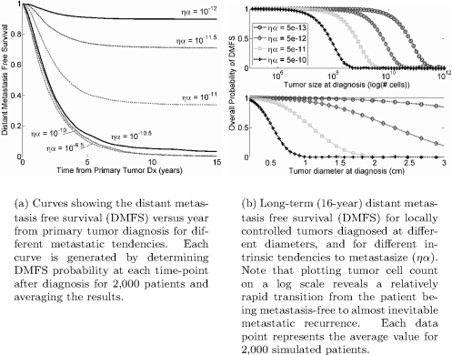
Some results from the basic Yorke model with complete local control. Note especially that the DMFS curve unexpectedly appears to approach an asymptotic curve as ryα increases. This is not seen when using the agent-based simulation model, as in Figure 7.4. Also, compare the prediction in (b) to that for drug resistance under the Goldie-Coldman model discussed in Chapter 9.
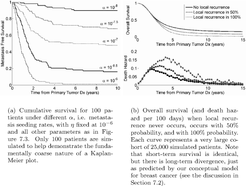
Kaplan-Meier survival curves generated using agent-based simulation of the Yorke model. Patient survival data is often reported and displayed using a Kaplan-Meier survival curve which gives the cumulative probability of the patient survival at any time. See exercise 7.4 for a method of generating such a curve.
To describe the metastases, let ρ(x, t) be density of metastatic colonies composed of x cells at time t. It is easy to see that ρ(x(t), t) is a constant if colonies do not disappear on their own. Hence it obeys a von Foerster (age-structured) model, as follows:
with initial and boundary conditions
Details of how one constructs and interprets such physiologically structured models can be found in chapter 4.
Initially there are no metastatic colonies of any size (condition (7.19a)). The (left) boundary condition (7.19b) is the rate of metastatic colony formation. All metastatic colonies begin with a single cell (at size 1). Integrating β(x)ρ(x, t) dx over all possible sizes gives the rate of seeding by existing metastases, while the primary tumor spawns new metastases at rate β(xp).
Finally, we assume that the rate of metastatic seeding is proportional to the number of tumor cells in contact with blood vessels. That is,
where k is the “colonization coefficient,” and ξ is the fractal dimension of the tumor vasculature. For a homogeneous vasculature servicing the entire tumor, ξ = 1, whereas a vasculature supplying only the outer tumor surface would have ξ = 2/3.
Iwata et al. considered both Gompertz and exponential growth functions for g(x) and found explicit solutions for both cases. Furthermore, they calibrated the model using data from a case of primary hepatocellular carcinoma with multiple liver metastases tracked by three serial CT scans. Interestingly, their calibration suggested that ξ was very close to 2/3, suggesting superficial vasculature.
This model allows the size distribution of metastatic colonies to be tracked through time. Because of its generality, it would be straightforward to explore the effect of therapeutic intervention on the size distribution of metastases. Adjuvant therapy could be easily modeled by adding a negative term to the growth function, g(x).
7.4.5 Thames model
Thames et al. [76] used a model to address the question of whether it is better to treat with chemotherapy before (“neoadjuvant” therapy) or after surgical resection of the primary tumor. They concluded that for early T1 cancer it is better to treat surgically first, but more advanced tumors may be better treated by neoadjuvant chemotherapy.
7.4.6 Other models
Chen and Beck [10] recently derived a mechanistic model for metastatic spread using superstatistics, which performed well against some SEER breast cancer survival data. Several other examples of stochastic models for metastatic spread can be found in [4, 42, 83]. Withers and Lee [80] discussed the implications of different tumor growth and metastasis dissemination kinetics on the distribution of metastases and the possibility of curative therapy.
7.5 Tumor dormancy hypothesis
Most continuous growth models for metastatic spread implicitly assume that tumors grow most rapidly in the earliest phases of their history, which follows naturally from the assumption of sigmoidal growth. Support for these assumptions rests on comparisons of model predictions to patient survival curves (e.g., Speer et al. [74] and Norton [53]). However, such data miss an important aspect of malignancy—cancer recurrence—that challenges the insightfulness of simple tumor growth models. In particular, the hazard function for both local and distant metastatic recurrence of breast cancer following treatment exhibits two peaks: a large one at about 18 months followed by a smaller peak at 60 months [17]. This pattern was first observed in data from the Milan National Cancer Institute for women treated by surgery alone [14], and has since been observed in other unrelated data sets [16]. It was not seen in the Bloom data [7], which has a single peak in mortality following diagnosis [18]. However, the Bloom data includes only untreated tumors and has a slight bias. So the two-peak mortality pattern appears to be a real characteristic of treated breast cancer.
On the basis of this pattern and other data challenging the continuous growth model for primary tumors, Demicheli, Retsky, and colleagues proposed the tumor dormancy hypothesis in 1997 [17, 69]. More recent reviews by this group (the hypothesis is essentially unchanged) can be found in [5, 16, 68].
This hypothesis proposes that metastatic colonies experience periods of dormancy that tend to end with removal of the primary tumor, at least transiently. Such stimulation of metastatic growth following primary tumor removal has been observed in a variety of cancer types in both animal models and human data-sets.
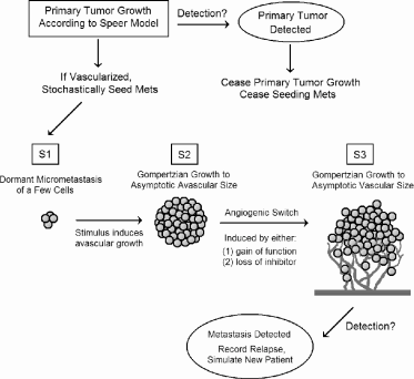
Demicheli and Retsky et al. proposed that distant micrometastases potentially experience two distinct phases of both dormancy and growth. Following seeding, the metastatic cells are in the first dormant state, S1, until some stimulus induces them to enter the first avascular growth phase, S2, where they grow until reaching the maximum avascular size, estimated to be between 2 × 10³ and 1.5 × 10⁵ cells. The first dormancy phase occurs when the tumor reaches diffusion limitation. (See Chapter 3.)
The final growth phase, S3, occurs when avascular colonies induce angio-genesis and switch to vascular growth. Demicheli and Retsky considered two possible mechanisms. The first was essentially evolutionary—metastatic cells initially lack the angiogenic phenotype and then switch to S3 by genetic alterations that confer angiogenic potential. The second possibility came from studies by Judah Folkman [30] and others suggesting that dormant mi-crometastases are held in an avascular state by secretions from the primary tumor, including endostatin and angiostatin. Removal of the primary relaxes the inhibition, allowing metastatic tumors to switch to an angiogenic phenotype, reigniting their growth.
Retsky et al. [69] simulated this hypothesis and compared the results to the Milan data. The simulation’s assumptions include the following:
- The primary tumor grows according to the Speer model for irregular breast cancer growth.
- At the onset of tumor vascularization, the primary tumor begins shedding metastatic cells.
- Larger tumors shed more cells than smaller tumors.
- New metastases always start in the first dormant state S1. They transition stochastically to the first growing state S2, where they expand according to the Gompertz model to their maximum avascular size. They then randomly transition to vascular growth, S3, which is also Gom-pertzian but with a much larger limiting size. Cells may also transition directly from S1 to S3.
- Upon clinical detection, the primary tumor is removed, and metastasis ceases.
- When a distant relapse occurs—that is, when a metastatic tumor in S3 reaches clinical detection—the simulation ends.
This model is depicted schematically in Figure 7.5. Retsky et al. did not present the model in a traditional mathematical framework. Doing so would be fairly straightforward and likely to clarify precisely how the model works. For example, it is only reported that metastases are seeded from the primary tumor at a stochastic rate: it is unclear what the distribution of this rate is or precisely how it depends upon the primary tumor size and node status. Presumably the stochastic process is Poisson, but how the rate is determined is unclear.
This model cannot be compared to clinical data without parametrization. Unfortunately, no details on the Gompertz growth parameters were published, other than that they were based on published values for animal (e.g., LoVo xenografts in nude mice in [15]) and human data (e.g., testicular cancer lung metastases in [13]). Details about the primary tumor growth model are also absent, as is a precise description of when in its history it begins to shed metastases. These weaknesses make it difficult to replicate or expand the results.
Retsky et al. use their model to distill the following conclusions and predictions:
- Simple stochastic transitions between the S1, S2, and S3 states can yield a two-peaked hazard function, but the first peak is unrealistically early and narrow compared to data.
- State transitions must be transiently enhanced following surgery to satisfactory fit the data. That is, a pro-growth stimulus following surgery spurs transition from S1 → S2, and a pro-angiogenic signal increases S2 → S3. Both may give an S1 → S3 transition.
- The first peak of relapses represents metastases whose growth was stimulated by primary tumor removal. Unperturbed micrometastases follow a slower growth pattern and give a broader second peak.
- More advanced tumors with metastasis-positive lymph nodes may respond best to chemotherapy, as they will be characterized by S2 → S3 transitions, implying that metastases will be vascularized and rapidly growing, and hence more responsive to chemotherapy.
- Smaller primary or larger, node-negative tumors are likely to be characterized by early metastases and S1 → S2 transitions following surgery. Since avascular tumors may respond poorly to chemotherapy, earlier detection may antagonize efficacy of chemotherapy. Long-term suppressive therapy is therefore a potential alternative to short-term chemotherapy.
The final two predictions are potentially important clinically. However, the notion that advanced tumors respond better to therapy because of a predominant S2 → S3 shift is questionable. Overall, it is likely that many S1 → S2 transitions would still occur. Thus, early stage metastases are likely to be equally present in more or less advanced tumors. Because continuous metastasis seeding by a primary tumor will always give a metastasis distribution with many early-stage metastases, early detection may antagonize chemotherapy in the short term, it still must improve the absolute benefit.
This model matches distant recurrence data fairly well and offers an interesting dynamical description of tumor dormancy, and indeed, it seems fairly certain that some departure from continuous growth kinetics must explain the extremely delayed recurrence seen in breast cancer. However, a major challenge to the conclusions and model is that, in the data, the two peaks of distant recurrence are paralleled by two peaks in local recurrence. How can we account for this? It may be that a similar tumor-host dynamic governs the growth of both occult metastases and residual primary tumor, and a transient pro-growth stimulus following surgery might affect both similarly. But residual local disease is unlikely to be described by the same S1 → S2 → S3 sequence as metastases.
The tumor dormancy hypothesis is an intriguing one and well worth further investigation. Therefore, it would be a valuable project to develop this model in an ODE setting that can more easily be expanded upon. Such a model could be used to more formally study the effect of adjuvant therapy on metastatic recurrence and relative efficacy for different primary tumor types. Also, the model should be expanded to explicitly consider residual local disease, and the relationship between local and metastatic recurrence could be further studied, as discussed above.
7.6 The hormonal environment and cancer progression
While we present no new models here, it is important to at least mention the role of hormones and breast cancer. Breast cancer, unlike most other solid malignancies, is characterized by extremely delayed recurrence that may occur up to two decades after apparently successful initial treatment. The hormonal environment probably plays a key role in such delayed recurrence along with mediating metastasis dormancy. The estrogen receptor (ER) promotes survival and mitosis in both normal and cancerous breast epithelium, and a majority of breast cancers are ER-positive at diagnosis, although a significant minority are not (perhaps 25%). A role for hormones in breast cancer progression and recurrence is supported by the success of hormonal therapy. Efficacy of oophorectomy (removal of the ovaries) was recognized as early as 1896 [26]. A more recent study showed that treatment using the ER antagonist tamoxifen reduces annual breast cancer mortality by 31% [23], and this benefit persists for up to 15 years, with continually increasing mortality divergence between treated and untreated groups. Further support comes from the Women’s Health Initiative, which in 2002 first showed that hormone replacement therapy (HRT) increases breast cancer risk. Significantly, while ER-positive tumors respond to hormonal therapy and have a better prognosis than ER-negative tumors, essentially no ER-negative tumor recurs more than five years after diagnosis, while the risk of recurrence in ER-positive tumors continues for 15 years or more [26].
Drawing on the work of Demicheli and others studying irregular breast cancer growth kinetics (see Section 7.5), Love and Niederhurber [52] endorsed a model suggesting that breast cancer is a disorder of host or environmental control, rather than simply “uncontrolled growth” that can only be stopped by annihilating tumors to the last cell. These authors also commented upon a surprising result: surgical oophorectomy in premenstrual women confers a significant survival benefit, yet this benefit appears to be restricted to women in whom surgery was performed during the luteal phase of the menstrual cycle. This observation led to the progesterone trigger hypothesis:
- High systemic levels of progesterone during the luteal phase support metastasis survival and vasculature;
- Sudden withdrawal of progesterone by luteal oophorectomy leads to mi-crometastasis arrest, perhaps by withdrawal of survival signals or regression of the vasculature.
Finally, we note that early pregnancy, which exposes the breast to sustained, high levels of estrogen, is strongly protective against breast cancer. This pattern seems puzzling if we view estrogen as a driver of cancer growth, as suggested by the adverse effects of HRT in later life. Possible explanations for the protective effect of estrogen include the following: (1) hormones of pregnancy drive a population of cells susceptible to neoplastic transformation to a mature, terminally differentiated state incompatible with malignant transformation, (2) early neoplastic cells are differentially sensitive to high levels of estrogen and are killed rather than supported, or (3) pregnancy alters sensitivity of cells to estrogen such that neoplastic cell survival cannot be supported [39].
7.7 The natural history of breast cancer and screening protocols
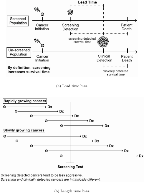
The impact of different screening protocols on cancer mortality has been the subject of various statistical and dynamical models. The efficacy of any cancer screening program can only be definitively established by randomized trials that track cancer mortality. Increases in survival time related to screening do not necessarily indicate a benefit to screening, due to lead-time and length-time biases. Lead-time is the survival time gained by detecting a disease earlier in its natural history. For example, assume a cancer is initiated at year 0 and destined to cause death at year 10. Further assume that the disease will become clinically evident at year 8, but screening detects it at year 5. In this case, screening increases survival by 3 years, even though the course of disease is unaffected by early detection. Length-time bias refers to the tendency of screening to detect diseases with longer natural histories. Figure 7.6 depicts these biases schematically. Both biases are inherent to screening and cannot be simply adjusted away. Therefore, it is difficult to know if earlier detection improves treatment efficacy without prospective trials that measure mortality.
Randomized prospective trials have, in fact, demonstrated that mammography screening reduces breast cancer mortality by perhaps 15–20% for women aged 40–74. Absolute benefit increases with patient age, and relative benefit may also reach its maximum in the 60–69 age group [61]. The appropriate use of screening remains controversial younger (aged 39–49) and older (over 74) women. For younger women, screening efficacy, while real, is very small (the number needed to screen to prevent one death is 1,904), and younger women may also be most likely to suffer false positives [61].
The two major risks associated with any screening test include false positives and overdiagnosis. Overdiagnosis, which may be considered the limiting case of length-time bias, refers to screen-detected cancers that would never have caused symptoms. Treating such a cancer can therefore only cause harm. Estimates of breast cancer overdiagnosis by mammography range from less than 1% to 30%, but most are in the 1–10% range [61]. Mammography in particular also exposes women to low-dose chest radiation.
7.7.1 Pre-clinical breast cancer and DCIS
Optimizing the value of screening is hindered by the fact that little is known about the natural history of pre-clinical breast cancer. Since the advent of mass mammography screening the incidence of ductal carcinoma in situ (DCIS) has increased dramatically. It now accounts for about 20% of new breast cancers, compared to less than 2% in the past, and this increase is largely attributable to mammography. DCIS is a neoplasm of ductal epithelial cells that has not penetrated the basement membrane to invade the surrounding stroma, although it may have spread widely within the duct lumen.
DCIS is generally believed to represent an early stage in the evolution of invasive carcinomas, and it shares many of the genetic and morphological characteristics of invasive disease. However, recent research has shown that not all cases of DCIS will progress to invasive cancer, and the proportion that do is unknown. Moreover, some more aggressive cancers may lack a recognizable in situ phase. Several studies have examined the rates of invasive carcinoma in women who received only a biopsy for DCIS and were initially misdiagnosed as having benign disease. These studies suggest that 14–53% of DCIS gives rise to invasive disease, but they had small sample sizes and considered only low-grade DCIS [25].
Welch and Black [79] reviewed seven autopsy series of women who died without evidence of breast cancer during life, and found the median prevalence of undetected DCIS to be 8.9%, although the prevalence was higher in studies that sampled more breast tissue (up to 14.7%). Furthermore, the prevalence was much higher in younger women. At the upper limit, 39% of women aged 40–49 had in situ disease, and another 12% had atypical ductal hyperplasia. This result suggests that a large pool of DCIS in younger women becomes depleted with increasing age. Depletion could occur either by spontaneous regression or progression to invasive cancer.
In accordance with Welch and Black’s results, other evidence points to markedly decreasing DCIS incidence detected by screening after age 70 [24]. In addition, invasive cancers in older women tend to be lower grade with more favorable prognostic factors [24, 25]. The cause of this shift in incidence and grade remains unclear at the time of this writing.
7.7.2 CISNET program
Cancer Intervention and Surveillance Modeling Network (CISNET) is a consortium of National Cancer Institute (NCI) sponsored investigators that use statistical modeling to improve our understanding of cancer control interventions in prevention, screening, and treatment and their effects on population trends in incidence and mortality.
Given that randomized trials have established a mortality benefit to breast cancer screening, we turn our attention to optimum screening schedules. Here, modeling comes into its own because it is logistically infeasible to test all possible screening regimes using prospective trials.
Two major approaches for modeling natural history in screening trials exist: (1) stochastic state-transition models, where tumors transition through a variety of pre-clinical phases, and (2) continuous growth models, which typically assume exponential or occasionally Gompertzian growth kinetics. These two approaches may also be combined.
The CISNET Breast Cancer Program, sponsored by the National Cancer Institute, was a collaborative effort to model the effect of screening and adjuvant therapy on breast cancer mortality and incidence between 1975 and 2000 [12]. Of the seven groups, six developed models for the natural history of breast cancer, and we review them here. The other used Bayesian simulation modeling [6], and we do not discuss it. The reader may also consult [12] for a comparative review of these models.
The CISNET models employ “discrete-event microsimulation,” in which individual patient life histories are simulated and the results aggregated. In general, all CISNET models have the following components:
- A patient population component, typically divided into birth cohorts.
- Breast cancer incidence component, where incidence rates by birth cohort are given as a model input.
- The tumor natural history component, including clinical cancer detection.
- The screening component, which takes into account changes over time in both mammography practice and the size threshold for tumor detection.
- Adjuvant treatment component, where the probability of a given therapy option being used and probability of tumor cure both depend on tumor characteristics at detection. The cure probabilities typically distilled from results of a meta-analysis of adjuvant therapy efficacy by the Early Breast Cancer Trialists Collaborative Group (EBCTCG).
All CISNET models included the following fixed inputs (base case inputs) [36]:
- Mortality in the population from causes other than breast cancer.
- Secular (long-term) trend in breast cancer incidence.
- Mammography screening dissemination.
- Adjuvant therapy dissemination.
The efficacy of adjuvant therapy and the probability tumors are estrogen-receptor positive are also generally determined by empirical data. This leaves parameters governing the natural history submodel and the threshold for detection by screening as free parameters determined by calibration to data. We will return to model calibration after we address the natural history submodels in the next section.
7.7.3 Continuous growth models
Four CISNET models [36, 75, 66, 43] described tumor natural history using continuous growth formalisms. Three used exponential growth without an explicit metastasis component [75, 66], while the Wisconsin group [36] used a more sophisticated Gompertzian model that explicitly included early tumor dormancy and regression, along with a simple model for metastatic spread. The latter work is an excellent example of how a good model confronted with data can be used to generate predictions about unobservable early tumor history.
MISCAN-Fadia model. The MISCAN computer model [40] is a state-transition model used to study screening for a number of malignancies. For example, Boer et al. [8] used a MISCAN breast cancer model to study disease progression from disease free through DCIS and on through four invasive cancer stages (T1a, Tab, T1c, T2+). Dwell-time in each stage was exponentially distributed, and probability of detection by screening depended upon stage.
In a modification of this basic approach, Tan et al. [75] altered the natural history component of the MISCAN framework to an exponential growth model, making tumor size the primary metric (rather than stage). Furthermore, they used the notion of a “fatal diameter” (“Fadia”): a tumor diameter unique to each patient at which the tumor becomes fatal; this diameter is (implicitly) assumed to be the point that fatal metastasis is initiated. This model assumes an initial spherical tumor of 0.1 mm diameter. The exponential growth rate is assigned randomly according to a log-normal distribution. The fatal diameter is selected from a Weibull distribution, and the survival time after reaching the fatal diameter is log-normally distributed. The tumor may be detected by screening or clinical detection of either the primary tumor or metastases. Screening and clinical detection of the primary tumor depend on tumor diameter thresholds, while clinical detection of metastases is a function of the time since a tumor became fatal.
Metastasis is not modeled other than to assume that tumor diameter is a marker for the probability of metastatic disease, i.e., the notion of the fatal diameter. DCIS is handled by the un-modified MISCAN DCIS submodel, which tracks incidence of two DCIS subtypes: (1) tumors that ultimately regresses, and (2) those that progress to an invasive cancer. Finally, adjuvant treatment is modeled by modifying a patient’s fatal diameter, implying a greater probability of cure at detection. The MISCAN-Fadia model is the simplest of the continuous growth models, and likely the least biologically reasonable.
Nevertheless, it matches SEER breast cancer incidence rates by tumor size reasonably well, with the exception of DCIS. From 1985 onward, the predicted DCIS incidence is increasingly too low. While the model mortality curve reflects the actual SEER mortality curve in shape, the model’s predicted mortality is too high.
Plevritis et al. model. Plevritis et al. [66] also assumed exponential growth for their natural history model, from the onset of invasive growth at a diameter of 2 mm until clinical detection. In particular,
where V (t) is tumor volume, and the inverse growth rate R is gamma distributed. Their model for local to regional to metastatic spread is proposed in terms of hazard functions. The hazard function for the time to the onset of regional (or nodal) disease, TN, is given by:
That is, there is some constant baseline hazard of regional spread, η0dt. The second term, η1V (t)dt, implies that the risk of regional spread increases in proportion to tumor volume. The o(dt) term represents un-modeled higher order terms.
The hazard function for the time of metastatic disease, TM, is very similar. The only difference is that regional disease must be established, i.e., TM ≥ TN, before distant spread can occur. Therefore, this model implicitly takes the view that metastatic disease spreads from the primary tumor in an orderly manner (Halsted model). The formal hazard function is:
The hazard function for clinical detection within a given time interval depends only on tumor volume, and the probability of detection is linearly related to tumor volume:
Finally, screening detection is modeled with a hazard function defined in terms of tumor volume intervals because screening occurs at discrete time intervals. The probability of detection by mammography is assumed to be proportional to tumor cross-sectional area, which is proportional to V2/3. Therefore, the hazard function for the threshold volume of detection, VTH is
A lower limit of detection is also imposed at a tumor diameter of 2 mm.
Adjuvant therapy efficacy is modeled by using published hazard ratio and varies by age and estrogen receptor status. The probability that a patient’s tumor is ER positive is determined by SEER data.
Significantly, Plevritis et al. did not attempt to model DCIS, and did not compare their model results to stage-specific SEER incidence rates, but only to the overall mortality curve. As in the MISCAN-Fadia model, the predicted mortality curve had the same shape as the SEER curve.
The negative results of these two models suggest that that DCIS and invasive cancer behave fundamentally differently. The MISCAN-Fadia model fails to predict increasing incidence of DCIS following introduction of widespread screening. The Plevritis et al. model does not attempt to model DCIS. It matched incidence rates well but overestimated mortality, which could not be resolved even if all tumors less than 1 cm in diameter were assumed to be DCIS destined to pose no risk. However, other explanations, such as increases in treatment efficacy, may explain Plevritis et al.’s mortality overestimate, so one should not read too much into these results.
Rochester model. Briefly, the Rochester model [43] considered the probability density function of the time of tumor initiation to be determined by a two-stage stochastic model of cancer incidence. Such models are discussed in Section 7.8.2. The random variable W gives the time from tumor initiation to detection, and its distribution is determined using continuous exponential tumor growth.
Wisconsin model. The Wisconsin group [36] simulated the female population of Wisconsin between 1950 and 2000, aged 20–100 years, divided into birth cohorts. This population includes 2.95 million women. The simulation was run in 6-month cycles, with a 25 year “burn in” period between 1950 and 1975 to establish breast cancer prevalence at 1975. Results were compared to measured 1975–2000 breast cancer rates.
The Wisconsin study’s natural history submodel assumes Gompertzian primary tumor growth with an initial occult mass with 2 mm diameter and an asymptotic diameter of 8 cm. The growth rate for individually simulated patients is selected from a gamma distribution, with mean and variance calibrated by data.
A nonhomogeneous Poisson process governed metastatic spread. Metastasis from primary tumor to local lymph nodes was modeled as a function of absolute tumor size and growth rate, as proposed by Shwartz [72]; that is, if n(t) is the rate at which groups of lymph nodes become positive, then
where the bi are all constants. In each 6-month simulation cycle, the number of new lymph node metastases is determined by random draw from a Poisson distribution with parameter n(t). While the assumption that regional spread correlates with both tumor size and growth rate is intuitively reasonable, there is no mechanistic basis for this rate function. The Yorke model (see Section 7.4.1) makes metastasis a function of tumor volume and growth rate in a much more mechanistic way.
A key feature of the Wisconsin model is that it considers DCIS to be an early stage of invasive breast cancer. Based on the primary tumor size and number of positive nodes, tumors are mapped to four historical SEER stages: (1) in situ (DCIS)—tumors without positive nodes and below a critical diameter, determined to be 0.95 cm, (2) locally invasive—tumors above the threshold for in situ disease, but with negative nodes, (3) regional spread—any tumor with 1–4 positive nodes, and (4) distant spread—5 or more positive nodes. Upon reaching the distant stage, the survival time distribution is derived from SEER data.
The probability that a screening test detects a tumor is assumed to be a function of tumor diameter and varies with time to reflect changes in mammography technology. Similarly, tumors emerge clinically with some probability determined by their diameter. The probability curve for clinical surfacing was determined in model calibration.
Therapy is modeled as a cure/no-cure process. That is, either a detected tumor is immediately eliminated or there is no effect at all upon the tumor’s natural course. The latter assumption is of course problematic, as non-curative therapy can still significantly extend survival time, but this is a reasonable first-approximation. Therapy is modeled as follows: baseline treatment, consisting of mastectomy with or without radiation was assumed to be applied to all patients. The probability of a cure from baseline treatment alone depends upon the stage. In addition to baseline treatment, one of five adjuvant therapies may be applied: (1) chemotherapy alone, (2) tamoxifen for 2 years, (3) tamoxifen for 5 years, (4) (cytotoxic) chemotherapy plus tamoxifen for 2 years, or (5) chemotherapy plus 5 years. The probability of each therapy is determined according to various published data and whether the tumor’s ER status is known. Survival probability is modified by each treatment according to a published meta-analysis [22].
The most important result of the model was its prediction that a significant fraction of occult-onset tumors grow only to a small size and ultimately regress. This conclusion reinforces other evidence that many DCIS tumors spontaneously regress (see the introduction to this section). We outline the steps leading to this prediction [36]. The rate of occult tumor onset, i.e. the rate at which 2 mm Gompertzian tumors are initiated, is estimated from the age-period-cohort (APC) model of Holford et al. [48] (a common CISNET input). However, since clinical incidence and occult onset are not the same, as some women may die of other causes before their cancer is detected, we define the “onset proportion” as the ratio of occult onset to clinical incidence:
We define the onset lag l as the average time between occult onset and clinical presentation. If all tumors are eventually detected, the tumor incidence rate in year Y is simply the onset rate in year Y − l. Taking into account the proportion of onset cancers that become incident, we have the following expression for the rate of occult onset in year Y :
This expression is valid only if all occult onset cancers are destined to become clinically incident. Fryback et al. [36] found that this expression does not yield the observed high rate of in situ disease following introduction of mass-screeing. It follows that not all occult onset cancers will become invasive. Therefore, we introduce a class of “limited malignancy potential” (LMP) tumors that grow to “Max LMP size,” remain at this size for “LMP Dwell time,” and then regress. Some fraction, the “LMP fraction,” of all occult onset tumors are randomly chosen to be LMP tumors. With this new class of tumors, we derive a new expression for the rate of occult onset as a function of the predicted clinical cancer incidence. First, redefine onset proportion as the ratio of non-LMP onset to clinical incidence:
Now, determine total onset rate using the following relations:
With some simple rearrangement we have the final expression for total occult tumor onset:
Thus, we have total onset in terms of the predicted clinical incidence rate, a model input, and two parameters with values determined by model calibration. The inclusion of a subset of small tumors destined to regress was needed to avoid depleting the pool of early tumors detected by screening in SEER data. It was also necessary to introduce two classes of hyperaggressive tumors to successfully match SEER data. In this case, some small fraction of onset tumors were assigned 4 nodes (regional stage) at 2 mm onset, while another fraction of tumors was assigned to the distant stage (5 nodes) at 2 mm onset.
Model calibration yields the following parameter values:
Thus, the model predicts that slightly less than half of all breast cancers that reach 2 mm in diameter are destined to regress by the in situ or early invasive stage of growth. This is in broad accord with studies tracking the incidence of invasive disease arising from in situ carcinomas misdiagnosed as benign [25] and autopsy studies revealing a surprisingly high prevalence of undiagnosed DCIS in younger women [79], as discussed earlier. We note that since a tumor of 2 mm diameter contains about 4.2 × 10⁶ cells (assuming 106 cells per mm3), it is unclear how modeling tumor initiation from a single cell would alter this prediction.
State-transition models. The so-called SPECTRUM model [55] and another by Lee and Zelen [51] describes tumor natural history as a series of stage transitions. Notably, the SPECTRUM model always underestimates DCIS incidence following screening, and the authors considered this indirect evidence that many DCIS never progress to invasive disease, and many screen-detected DCIS may be over-treated.
7.7.4 Conclusions and optimal screening strategies
The SPECTRUM and MISCAN-Fadia models fit clinical data well, with the exception of the increasing DCIS incidence following widespread screening. The Wisconsin model predicts that a fraction of DCIS is destined to regress. These results, along with previously discussed autopsy series [79], suggest that a significant fraction of DCIS not only never surface clinically, but fully regress.
The CISNET models were also recently applied to a more pressing clinical problem: the optimal mammography screening strategy [54]. A set of screening strategies that varied by starting and stopping age (e.g. 40–84 vs 50–74) and screening interval, either annual (A) or biennial (B), were tested using six of the CISNET models. A screening strategy is considered “inefficient” or “dominated” if it both (1) results in worse health outcomes (mortality reduction and increase in life-years), and (2) requires more resources (mam-mographies per 1000 women) than any other strategy considered. Across all models, eight strategies were found to be non-dominated. All but one (A40– 84) used biennial screening and all but two began screening at age 50 rather than age 40.
This work further found that screening women beginning at age 40, rather than age 50, does decrease mortality, but only by about 3%. Due to the low incidence of cancer in the 40–49 age group, the absolute benefit is therefore very small, perhaps less than harm due to the screening procedure. Moreover, more resources are consumed and more false positives occur. Also, mortality is predicted to decrease more by screening older patients (over 74) than by screening younger women, but screening younger women should add more overall life-years (total years of life gained).
These results helped motivate a recent statement by the U.S. Preventive Services Task Force [77] that recommends (1) against routine mammography for women aged 40–49, and (2) biennial screening for women of ages 50– 74. This recommendation to reduce screening has been very controversial and in some cases vehemently condemned. While certainly debatable, the recommendations are based on data, and represent a significant contribution of modeling to an important clinical problem.
7.8 Cancer progression and incidence curves
Most models we have discussed so far consider cancer growth under a constant parameter regime. Yet, cancer growth rates evolve. Therefore, the parameters describing tumor growth kinetics almost certainly cannot remain constant over the entire tumor history. However, simple Gompertzian models in which tumors, after initiation, progress according to constant parameter values most naturally assume cancer as an essentially “one-hit process.” However, it is well known that most tumors arise from multiple “hits” to their genomes. So we have another challenge to the simple Gompertz view of tumor growth.
7.8.1 Basic multi-hit model
Cancer incidence increases dramatically with age, a fact initially regarded as inconsistent with the hypothesis that cancer arises from mutation in normal cells [62]. If clinical cancer is sparked by a single aberrant mutation, then age-specific cancer incidence rates should be constant, at least among adults if there is a significant delay between cancer initiation and clinical presentation. However, the epidemiological evidence shows clearly that age-specific incidence is not constant, an observation that motivated the first explicit multi-hit models, which we now discuss.
By the early 1950s it was well known that many carcinogenic agents are also mutagenic, and there is typically a latency period between carcinogen exposure and clinical cancer. In 1953, Nordling first proposed that malignant transformation of a single cell requires a sequence of multiple mutations [62]. He argued that if a single mutation sufficed, then cancer incidence would be the same for all ages. If two mutations were required, then the number of cells carrying a single “hit” (cancer-causing mutation) would increase in direct proportion to age, and so the incidence (requiring the second hit) would be directly proportional to age. If three hits were needed, incidence would increase as the second power of age, and so on. Nordling then examined cancer mortality data for adult men in the U.K., excluding children and the very old, and observed that mortality increased with the sixth power of age, implying that, on average, seven mutations are necessary.
Armitage and Doll [1], in 1954, reached a similar conclusion using more rigorous probabilistic reasoning. If malignant transformation requires r mutations, the ith mutation occurs with probability pi per unit time, and if these mutations must occur in a particular order, then the probability that a cell becomes malignant (acquires the rth) in the time interval (t, t + dt), is
(If the mutations can occur in any order, the following result still holds.) It follows that the cancer incidence rate, I(t), is proportional to the (r − 1)th power of time (i.e. age); i.e.,
where k is constant. Taking the logarithm of both sides yields
which implies that a log-log plot of cancer incidence versus age should be a straight line with slope (r − 1). Data from nine different types of cancer gave slopes between 4.97 and 6.48. The slope for colon and rectal cancer came out to be approximately five, suggesting six rate-limiting steps for this particular neoplasm.
Armitage and Doll’s model has become the classic multi-hit model for cancer incidence. It assumes that intermediate mutations confer no selective advantage or functional change to the cell, and that cancer arises only after all hits have occurred. In this case, mutation order cannot matter, and all mutations are mathematically equivalent. However, if mutations confer differential selective advantages, then mutation order does matter because selection dynamically alters the pool of cells which may be mutated. Therefore, there is a slight conflict between Armitage and Doll’s original analysis, which assumed a particular order is necessary, and the actual model which implies that order does not matter.
We can also recast the basic multi-hit model as a simple system of differential equations, as done by Frank [31]. Letting xi(t) represent the number of cells with i mutations at time t, Frank proposed the following simple model:
where ui is the rate at which cells with i mutations mutate. This formulation helps point out some issues with rate parameters. It is natural to assume that transition rates should be the same, at least in first approximation, since one may expect genes to mutate at roughly the same rate. However, the basic multi-hit model requires that mutations are unordered (see discussion above). Since the number of genes available for mutation decreases with each hit, transition rates must vary among stages.
If the order of mutations does matter, then transition rates will be constant (at least under the assumption that mutations never occur out of sequence). This may be the better assumption, at least in some cases. For example, colon carcinoma seems to exhibit a preferred progression of genetic changes during transition from dysplasia to clinical cancer. Interestingly, the slope of the log-log plot is constant whether or not the ui vary, implying that incidence curves give no information on whether mutations are ordered or not.
This discussion highlights the complexities introduced when mutations confer selective advantage. In such cases, one must be very careful to define the mutation mechanism and transition rates among mutant states correctly. Moreover, if mutation order is indeed unimportant, the rate at which pre-cancerous lesions evolve toward malignancy may reach its maximum at an intermediate number of mutations, but slow as more hits are acquired.
7.8.2 Two-hit models
We now turn to another model by Armitage and Doll, this one from 1957 [2]. Here the authors do consider the role of selection in a pre-cancerous tumors. They showed that such selection can yield cancer incidence proportional to the sixth power of age with only two genetic hits required for cancer. The model considers the influence of two carcinogenic agents. The first acts as an initiator, and cells acquire the initial mutation at a rate proportional to dose. These precancerous cells undergo exponential clonal expansion and are susceptible to malignant transformation by the second agent. Let d1 and d2 be the doses of initiating and transforming agents, respectively, and nt represent the number of precancerous cells at time t after exposure to the first dose. Then
Relation (7.40) expresses the exponential expansion of premalignant cells following exposure to the initiating agent. Using probabilistic arguments, Armitage and Doll arrived at the following equation for cancer incidence:
where N is the number of persons at risk for the first mutation and, as before, I(t) is cancer incidence at time t. Here, p1 is the probability per unit time that a normal cell undergoes the first mutation and is proportional to d1; p2 is the per unit time probability of the second mutation and is likewise proportional to d2.
We arrive at expression (7.42) by the following arguments. Suppose a clone has undergone the initiation step at time t − T, but has not transformed by time t. Then the clone transforms to malignancy with probability p2 exp(kT) per unit time. The probability that the second change occurs in the small time interval (t, t + dt), but not before, is therefore approximately
Transitions from the intermediate class to malignancy is governed by a Poisson process with a non-constant rate proportional to the number of intermediate cells. Therefore, the transition rate parameter on the interval (0, T) is λ = p2 exp(kT). It follows from probability theory that:
The probability of the second change in (t, t + dt) is
Now, we need the probability that the first change occurs in the interval (t − T, t − T + dT). The time to the first mutation is exponentially distributed with parameter p1, so
It follows from the Taylor series of the exponential that, if p1dT is small, we can approximate 1 − exp(−p1dT) as
The probability we seek is therefore the product of equations (7.45) and (7.47) (given with some rearrangement):
All that remains is to integrate over time between the first and second mutations, T, to get the final probability of a second mutation in the interval (t, t + dt):
We recover relation (7.42) by multiplying the right-hand side of equation (7.49) by N, the number of persons at risk.
This model successfully matched mortality data for stomach, intestine, colorectal, and pancreatic cancer for persons aged 25–74 years. In many hormone-dependent cancers, such as breast and ovarian cancer, the slope of the incidence curve decreases in later life. Armitage and Doll suggest that this model could be made to match these cancers as well if hormones were promote clonal expansion of singly mutated cells.
From equation (7.42), we can make several predictions concerning cancer incidence. First, it should increase linearly with exposure to the initiating carcinogen and increase exponentially with exposure to the transforming carinogen. Furthermore, as t → ∞, we have I → Np1. Thus, the model predicts that all age-incidence curves should eventually become constant, which accords well with the observation that cancer incidence curves tend to flatten with age.
Finally, we note that as with the basic multi-hit model, we may also reformulate this model in terms of differential equations:
In this case, I(t) ∝ dx2/dt.
Retinoblastoma, a rare childhood tumor of the eye, has been examined in the context of two-hit models by Kundson and colleagues, beginning with a seminal paper in 1971 [50]. This tumor often shows a hereditary pattern, but can also arise spontaneously. In either case, both copies of a key tumor-suppressor gene, called Rb, must be inactivated for cancer to occur. Incidence data and probabilistic arguments led Knudson et al. to hypothesize that hereditary retinoblastoma arises when one of the Rb genes is already mutated in the germ line (lineage of cells that produces gametes). Therefore, they hypothesize that only one additional hit is necessary to spark the cancer. In contrast, spontaneous cases would require both alleles to be inactivated, implying a two-hit incidence pattern. Beyond being among the first cancers to which the two-hit etiology has been applied, retinoblastoma also provided the first evidence for tumor suppressor genes. Frank also recently revisited this hypothesis using a simple mathematical model [32].
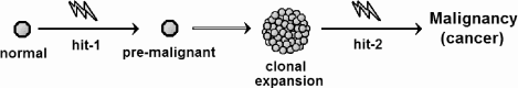
Following Knudson et al.’s lead, Moolgavkar, Knudson, and others have developed many two-hit stochastic models for tumor growth [59, 58]. In these models, healthy stem cells transition via mutation to intermediate cells with a slight proliferative advantage. This expanding clone may then undergo a second mutation to become malignant. Like the model of Armitage and Doll, tumor initiators cause the first transition, while tumor promoters increase the proliferation rate of intermediate cells without inducing mutation [58]. This two-hit framework, sometimes referred to as the two-stage clonal expansion model (TSCE), has been widely used to model carcinogenesis. The TSCE is essentially equivalent to a common conceptual framework called the initiation-promotion-progression “model.”
7.8.3 The case of colorectal cancer
While two-hit or initiation-promotion-progression models are popular, they are almost certainly too simple. Most adult carcinomas require multiple genetic modifications. Colorectal cancer, for which the key molecular events driving progression are reasonably well defined, provides an example.
The morphologic progression from early adenoma to invasive cancer is driven by genetic and genomic instability that arises early in this tumor’s evolution; it characterizes nearly all colorectal carcinomas and adenomas. Two major forms of instability are observed: (1) chromosomal instability (CIN) which leads to aneuploidy, present in about 85% of cases, and (2) microsatel-lite instability (MSI), associated with defective DNA mismatch repair (MMR) and present in 15% of cases. These two phenomena tend to be mutually exclusive [81], suggesting that genetic stability plays an important functional role in carcinogenesis irrespective of its molecular basis.
A set of key genetic changes that occur in cancers arising by CIN, termed the “traditional pathway,” were characterized in 1988 by Vogelstein, Fearon, and colleagues [78, 27] based on molecular analysis of 172 colorectal cancers. Morphologically, these lesions typically progress through the following stages: (1) normal epithelium, (2) aberrant crypt focus (ACF), (3) early adenoma, (4) late adenoma, (5) invasive cancer, and finally (6) metastatic disease.
Genetically, the earliest change is either loss of the APC gene on chromosome 5q or a mutation of the K-ras gene, which gives rise to a dysplastic ACF. While the K-ras mutation may actually occur first [81], sources traditionally list APC as the initiating mutation [27]. Inactivation of APC leads to loss of proliferation suppression by the Wnt signaling pathway and may contribute to the development of CIN. Further progression to invasive cancer is associated with mutations in the K-ras oncogene, loss of 18q, causing inactivation of DCC, SMAD2, and SMAD4 tumor suppressor genes, and loss of 17q, which causes p53 tumor suppressor inactivation (Figure 7.8). This set of genomic alterations is unlikely to be sufficient to cause cancer. A number of other genetic and epigenetic alterations are also associated with cancer progression, and non-invasive adenomas with all four changes exist [27]. While there is a preferred order for these changes, their net accumulation is likely more important than the order [27]. The apparent ordering may be a function of the selective advantage or genomic instability conferred by individual mutations.
![]()
Traditional pathway of colorectal tumorigenesis. Depicted are the canonical genetic hits associated with morphological progression.
Most tumors do not actually harbor all canonical changes of the traditional pathway [81], suggesting that they arise through functional changes in phenotype. The traditional pathway may (partially) represent only one of many ways to generate the same phenotype. This view accords well with the hallmarks of cancer, which include a limited number of rate-limiting steps generating malignant phenotypes. But a given phenotype may be conferred by a variety of genotypes.
Thus, from the biology we can see that a two-hit model clearly cannot describe colon cancer, and some form of a multi-hit model is required. Recall from above that Armitage and Doll’s 1954 work suggested that six mutations are necessary for colon cancer. However, the fact that adenomas arise at all and accumulate genetic changes as they grow argues for a selective advantage conferred to pre-cancerous clones. It is generally accepted that adenomas advance by successive rounds of clonal expansion, where more fit clones out-compete the existing adenoma population [27]. Therefore, the basic multi-hit model without clonal expansion cannot be applied either. A clonal expansion model similar to that proposed by Frank [31] may be more appropriate. By modifying mutation rates it could also be made to handle genetic instability.
Several recent mathematical models have been used to study colon cancer [53, 65, 57]. Nowak et al. [65] studied a simple mutation network to determine the role of CIN in APC inactivation in early colon cancer. Later, Michor et al. [57] used a somewhat similar model to study CIN’s role in tumor suppressor inactivation in a more abstract setting. While Nowak et al. used stochastic methods to study their model which we do not cover here, we briefly outline the studied mutation network, parametrization, and model conclusions.
It is frequently the case that one copy of APC is inactivated by a point mutation in the gene, while the second is lost via a gross chromosomal deletion, a so-called loss-of-heterozygosity (LOH) event. Chromosomal instability increases the rate of LOH by orders of magnitude; therefore, induction of CIN may be the rate-limiting step in tumor evolution, rather than the LOH event itself. Nowak et al.’s model considered a population of colon crypt cells in two basic classes: with and without CIN. Let xi, i ({0, 1, 2} be the mass of cells in the first class (without CIN) with i inactivated copies of APC. Similarly, y0, y1, and y2 be CIN cells with 0, 1, and 2 inactivated copies of APC. They assume that active APC genes in all cells become inactivated by point mutations at rate u ≈ 10−7 per cell division. Transition from i = 0 to i = 1 therefore occurs at rate 2u (to account for the two ways in which this transition can occur). The second APC gene becomes inactivated either by a second point mutation at rate u, or by LOH, assumed to occur in non-CIN cells at rate p0. LOH in CIN cells arises at a much higher rate, p > p0, estimated to be about 0.01 per cell division. Finally, they allow caretaker genes (the products of which maintain genomic stability) to mutate, resulting in a transition from non-CIN to CIN. Assuming nc caretaker genes exist, then the transition xi → yi occurs at rate 2ncu.
Based on their simulations, Nowak et al. [65] concluded tha CIN typically arises early in tumorigenesis. However, since CIN alone decreases cell fitness, then it probably follows inactivation of the first APC gene, while the second most often is deleted via LOH. However, if CIN is neutral or advantageous, then CIN may be the initiating event in tumorigenesis. In either case, the model suggests that CIN is an early and rate-limiting event in tumorigenesis. Michor et al. [57] reach essentially the same conclusion.
Luebeck and Moolgavkar [53] extended 2-hit colon cancer incidence models to include 3, 4 or 5 premalignant steps. The four-stage model best matched SEER data on colon cancer incidence. Moreover, their best-fit parameter estimates suggested that colon cancers are initiated by two rare genetic events (e.g. mutations) followed by a single high-frequency event, giving rise to clonal expansion of the premalignant population from which the final event sparks malignancy.
This prediction coincides with Nowak et al.’s [65] suggestion that a point mutation in APC is followed by induction of CIN. The two slow steps predicted by Luebeck and Moolgavkar may be mutation of one APC and onset of CIN. Following CIN, the tumor likely rapidly inactivates the second APC and begins clonal expansion. A final p53 mutation, which is likely to occur in short order following CIN, may be the Luebeck and Moolgavkar’s fourth rate-limiting step. We now have a plausible reconciliation between the biological necessity that more (and probably far more) than four mutations are necessary to yield invasive cancer and the epidemiological agreement between a four-stage model and colon cancer incidence. This view also suggests that early tumor formation may be dominated by rare, stochastic genetic events; however, following CIN and the onset of rapid genome derangement, growth may be modeled reasonably well by deterministic kinetics.
7.8.4 Multiple clonal expansions
One important aspect of tumorigenesis that we have not yet encountered in tumor models is multiple rounds of clonal expansion. Such a behavior was considered by Frank [31]. He modified the continuous version of the basic multi-hit model (see above) to consider logistic growth of each clone individually. Clones grew independently with a limiting size that depended only on the clone’s size, not the tumor’s, an assumption that can be challenged on biological grounds.
Nevertheless, this model yields theoretical cancer incidence curves that match several observed phenomenon. In particular, it predicts the flattening log-log incidence curve that occurs in advanced age. Frank termed this phenomenon a decrease in the “age-specific acceleration” of cancer.
7.8.5 Smoking and lung cancer incidence
We close by mentioning the case of lung cancer and smoking. Cigarette smoke is generally believed to act as both tumor initiator and promoter. That is, it directly induces genetic mutations and promotes a host environment permissive of neoplasia. Smoking’s enhancement of cancer risk is well documented, and its effect on risk for ex-smokers has been tracked in large data-sets that provide excellent opportunities to test the predictive ability of multi-stage models.
After cessation of smoking, the excess risk for lung cancer declines fairly rapidly, and continues to decline for about two decades. However, the absolute cancer risk declines slightly and remains fairly static, or “frozen,” over time.
The basic multi-hit model was first applied to this problem by Doll in 1978 [21], who concluded that smoking affects the first stage and a late, perhaps the last, stage. (Later work generally assumes it affects the penultimate stage.) These conclusions are supported by data. That smoking affects an early step in tumor progression follows from the fact that, when cancer incidence is plotted against time of exposure, both smokers and non-smokers show the same power relationship. That smoking accelerates a later step is implied by the observed rapid reduction in cancer risk after smoking cessation. Finally, Doll observed a quadratic relationship between the dose rate (i.e., cigarettes smoked per day) and incidence, again suggesting that two stages are affected.
In related work, Brown and Chu [9] used a multi-hit model to estimate the rates of the two events affected by smoking. Their results predicted that cigarette smoking increases the rate of the late event by twice as much as it does the early event. They concluded that the greater part of total cancer risk is due to smoking’s effect on the penultimate event.
Importantly, the multi-hit models of smoking’s effect on cancer risk tend to predict, contra the data, that when a person stops smoking, the excess lung cancer risk continues to rise. This is discussed extensively by Freedman and Navidi [35]. They predicted the existence of a mechanism to repair smoking-induced lesions as a possible explanation for the reduction in excess risk and the failure of multi-hit models [35].
More recently, several two-stage clonal expansion models [45, 44, 19] have been applied to the problems of lung cancer incidence and smoking. All have concluded that smoking acts primarily as a tumor promoter. It may also be an initiator, and initiation and promotion may interact synergistically to increase risk [44].
7.8.6 Summary
While we have largely focused on kinetic models in this chapter, we have introduced multi-hit epidemiological models because of their historical importance on understanding the etiology of cancer, and because they address a key facet of the natural history of cancer. We are also motivated to examine such models because the genetic changes that occur in cancer etiology must necessarily affect tumor growth dynamics.
Very different genetic hit models can give similar cancer incidence curves, implying that while incidence curves have been instrumental to understanding the genetic basis for cancer, they cannot tell us the whole story. It remains an open question how mutations give rise to gross tumor growth kinetics. It is generally accepted that repeated rounds of clonal expansion drive both genetic and morphologic evolution, at least in the case of colon cancer. But aside from an intermediate period of exponential growth for two-stage models, the genetic hit models do not address growth kinetics. The models of Nowak et al. [65] and Luebeck and Moolgavkar [53] suggest that kinetic models may describe tumor growth reasonably well following CIN, after which rare genetic events may no longer be rate-limiting (although further genetic changes would continue to be necessary). Nevertheless, kinetic models of gross tumor growth have yet to be systematically unified with models of molecular etiology of cancer.
7.9 Exercises
Exercise 7.1: Show that if
then
where the asymptotic tumor size is N∞. Assume the tumor is detected at size ND at time TD. Show that
Exercise 7.2: Let P be a constant. Show that the solution of
is
Exercise 7.3: The Yorke model is stochastic and too complex to be easily amenable to analysis. Therefore, to gain insight implement and study the basic model computationally:
- Implement the basic model for primary tumor growth and metastasis seeding. Generate the distant metastasis free survival curve for a set of simulated patients, assuming no local recurrence occurs. For a more challenging extension, add local recurrence.
- (a) We assume that the metastases have a different growth rate than the primary tumor, randomly drawn from the same distribution. Also, the model construction necessitates that all metastases have the same growth rate. Are these realistic assumptions?
- (b) From Figure 7.3(a), we see that the DMFS curve approaches an asymptote. This is obviously not realistic. What model assumption could be responsible for this behavior, and how might it affect predictions?
Exercise 7.4: In the clinical medicine literature, patient survival data is widely reported and displayed using Kaplan-Meier survival curves. Such a curve gives the cumulative probability of survival at any time, and can be approximated (but not replicated) by the DFMS curves of the basic model. We note that Kaplan-Meier plots are valuable because they can incorporate censoring, i.e. patient loss. To generate such curves using a model it is not enough to know the probability of death at a given time: the individual times of death must be known exactly. Implement a simulated version of the Yorke model and use it to generate a Kaplan-Meier curve. A very brief pseudocode follows:
1. Pre-define the simulation time as (0, T_max).
2. For all N simulated patients:
1. Randomly determine primary tumor growth parameter.
2. Calculate time to detection, T_D.
3. Divide the pre-clinical history, t = (0, T_D) into Q discrete steps of length T_s.
4. At every time-step, calculate the number of metastatically-capable cells, m(t), as a function of the number of primary tumor cells:
m(t) = (1 −n(t)^(-alpha)) * n(t). Also:
A. The number of mets successfully seed during each time-step is Poisson-distributed with parameter: (eta) * m(t) * T_s.
B. Randomly seed metastases with unique, random growth rates. Calculate the time to detection and time to death for each met. If this is the minimum, store this value.
C. Store the time of met seeding and growth rate for all mets.
5. Use the data from (C) to determine the total metastatic burden at all times. Use this to determine if death occurs at an earlier time than previously determined.
6. Have local recurrence randomly occur with some probability.
7. If recurrence happens, follow a similar algorithm to that above.
3. Discretize the time domain (0, T_max) and, from the individual patient data, store the total number of patients still alive and recurrence-free at each time-point.
4. Plot the fraction of patients still alive at each time-point as a stair-plot, giving a Kaplan-Meier plot.
- Use the simulated model to determine how sensitive survival (in terms of both the shape of the cumulative survival and long-term survival) is to the following:
- (a) Tumor size at diagnosis.
- (b) Intrinsic metastatic potential, as measured by α and η.
- (c) The probability of local recurrence.
- (d) The residual tumor size following local treatment.
- (e) Tumor growth rate (parameter b).
- Following 1(e), all else being equal, do faster-growing tumors have a better or worse prognosis than slow-growing tumors? Note that, clinically, faster tumor growth is clearly correlated with poorer survival. What does this suggest about the validity of the model?
- The degree to which disease free survival (DFS) (i.e. the minimum of DMFS or time to local recurrence) correlates with survival after recurrence (SAR) is controversial. How well do these metrics correlate under different probabilities of local recurrence?
Exercise 7.5: The current model assumes that it takes only one genetic hit for cells to become metastatically capable. Biologically, what capabilities must a cell acquire to enter the bloodstream and survive to found a distant colony? Are these likely to be conferred by a single hit? Develop an alternative model in which two or more hits are required for metastatic capability.
Exercise 7.6: Implement a cancer-screening program under the Yorke model. That is, for every patient, during the pre-clinical period, t < TD, at regular intervals (say, every year) check to see if the tumor has passed some more smaller threshold size, , and if it has, initiate treatment. Characterize the effect of screening on both short-term and long-term survival under this model.
References
[1] Armitage P, Doll R: The age distribution of cancer and a multi-stage theory of carcinogenesis. Br J Cancer 1954, 8:1–12.
[2] Armitage P, Doll R: A two-stage theory of carcinogenesis in relation to the age distribution of human cancer. Br J Cancer 1957, 11:161–169.
[3] Barbolosi D, Benabdallah A, Hubert F, Verga F: Mathematical and numerical analysis for a model of growing metastatic tumors. Math Biosci 2009, 218:1–14.
[4] Bartoszyński R, Edler L, Hanin L, Kopp-Schneider A, Pavlova L, Tsodikov A, Zorin A, Yakovlev AY: Modeling cancer detection: Tumor size as a source of information on unobservable stages of carcinogenesis. Math Biosci 2001, 171:113–142.
[5] Baum M, Demicheli R, Hrushesky W, Retsky M: Does surgery unfavourably perturb the “natural history” of early breast cancer by accelerating the appearance of distant metastases? Eur J Cancer 2005, 41:508–515.
[6] Berry DA, Inoue L, Shen Y, Venier J, Cohen D, Bondy M, Theriault R, Munsell MF: Modeling the impact of treatment and screening on U.S. breast cancer mortality: A Bayesian approach. J Natl Cancer Inst Monogr 2006, 36:30–36.
[7] Bloom HJ, Richardson WW, Harries EJ: Natural history of untreated breast cancer (1805-1933). Comparison of untreated and treated cases according to histological grade of malignancy. Br Med J 1962, 2:213–221.
[8] Boer R, de Koning HJ, van der Maas PJ: A longer breast carcinoma screening interval for women age older than 65 years? Cancer 1999, 86:1506–1510.
[9] Brown CC, Chu KC: Use of multistage models to infer stage affected by carcinogenic exposure: Example of lung cancer and cigarette smoking. J Chronic Dis 1987, 40:171S-179S.
[10] Chen LL, Beck C: A superstatistical model of metastasis and cancer survival. Physica A: Stat Mech Appl 2008, 387:3162–3172.
[11] Clarke M, Collins R, Darby S, Davies C, Elphinstone P, Evans E, Godwin J, Gray R, Hicks C, James S, MacKinnon E, McGale P, McHugh T, Peto R, Taylor C, Wang Y; Early Breast Cancer Trialists’ Collaborative Group (EBCTCG): Effects of radiotherapy and of differences in the extent of surgery for early breast cancer on local recurrence and 15-year survival: An overview of the randomised trials. Lancet 2005, 366:2087–2106.
[12] Clarke LD, Plevritis SK, Boer R, Cronin KA, Feuer EJ: A comparative review of CISNET breast models used to analyze U.S. breast cancer incidence and mortality trends. J Natl Cancer Inst Monogr 2006, 36:96– 105.
[13] Demicheli R: Growth of testicular neoplasm lung metastases: Tumor-specific relation between two Gompertzian parameters. Eur J Cancer 1980, 16:1603–1608.
[14] Demicheli R, Abbattista A, Miceli R, Valagussa P, Bonadonna G: Time distribution of the recurrence risk for breast cancer patients undergoing mastectomy: Further support about the concept of tumor dormancy. Breast Cancer Res Treat 1996, 41:177–185.
[15] Demicheli R, Foroni R, Ingrosso A, Pratesi G, Soranzo C, Tortoreto M: An exponential-Gompertzian description of LoVo cell tumor growth from in vivo and in vitro data. Cancer Res 1989, 49:6543–6546.
[16] Demicheli R, Retsky MW, Hrushesky WJ, Baum M: Tumor dormancy and surgery-driven interruption of dormancy in breast cancer: Learning from failures. Nat Clin Pract Oncol 2007, 4:699–710.
[17] Demicheli R, Retsky MW, Swartzendruber DE, Bonadonna G: Proposal for a new model of breast cancer metastatic development. Ann Oncol 1997, 8:1075–1080.
[18] Demicheli R, Valagussa P, Bonadonna G: Does surgery modify growth kinetics of breast cancer micrometastases? Br J Cancer 2001, 85:490– 492.
[19] Deng L, Kimmel M, Foy M, Spitz M, Wei Q, Gorlova O: Estimation of the effects of smoking and DNA repair capacity on coefficients of a carcinogenesis model for lung cancer. Int J Cancer 2009, 124:2152–2158.
[20] Devys A, Goudon T, Lafitte P: A model describing the growth and the size distribution of multiple metastatic tumors. Disc Cont Dyn Sys B 2009, 12:731–767.
[21] Doll R: An epidemiological perspective of the biology of cancer. Cancer Res 1978, 38:3573–3583.
[22] Early Breast Cancer Trialists’ Collaborative Group (EBCTCG): Systemic treatment of early breast cancer by hormonal, cytotoxic, or immune therapy. 133 randomised trials involving 31,000 recurrences and 24,000 deaths among 75,000 women. Lancet 1992, 339:1–15.
[23] Early Breast Cancer Trialists’ Collaborative Group (EBCTCG): Effects of chemotherapy and hormonal therapy for early breast cancer on recurrence and 15-year survival: An overview of the randomised trials. Lancet 2005, 65:1687–1717.
[24] Erbas B, Amos A, Fletcher A, Kavanagh AM, Gertig DM: Incidence of invasive breast cancer and ductal carcinoma in situ in a screening program by age: Should older women continue screening? Cancer Epi-demiol Biomarkers Prev 2004, 13:1569–1573.
[25] Erbas B, Provenzano E, Armes J, Gertig D: The natural history of ductal carcinoma in situ of the breast: A review. Breast Cancer Res Treat 2006, 97:135–144.
[26] Eroles P, Bosch A, Bermejo B, Lluch A: Mechanisms of resistance to hormonal treatment in breast cancer. Clin Transl Oncol 2010, 12:246– 252.
[27] Fearon ER, Vogelstein B: A genetic model for colorectal tumorigenesis. Cell 1990, 61:759–767.
[28] Fisher B: The evolution of paradigms for the management of breast cancer: A personal perspective. Cancer Res 1992, 52:2371–2383.
[29] Fisher B, Slack N, Katrych D, Wolmark N: Ten year follow-up results of patients with carcinoma of the breast in a co-operative clinical trial evaluating surgical adjuvant chemotherapy. Surg Gynecol Obstet 1975, 140:528–534.
[30] Folkman J: Tumor angiogenesis: Therapeutic implications. N Engl J Med 1971, 285:1182–1186.
[31] Frank SA: Age-specific acceleration of cancer. Curr Biol 2004, 14:242– 246.
[32] Frank SA: Age-specific incidence of inherited versus sporadic cancers: A test of the multistage theory of carcinogenesis. Proc Natl Acad Sci USA 2005, 102:1071–1075.
[33] Franks SJ, Byrne HM, Mudhar HS, Underwood JC, Lewis CE: Mathematical modelling of comedo ductal carcinoma in situ of the breast. Math Med Biol 2003, 20:277–308.
[34] Franks SJ, Byrne HM, Underwood JC, Lewis CE: Biological inferences from a mathematical model of comedo ductal carcinoma in situ of the breast. J Theor Biol 2005, 232:523–543.
[35] Freedman DA, Navidi WC: Ex-smokers and the multistage model for lung cancer. Epidemiology 1990, 1:21–29.
[36] Fryback DG, Stout NK, Rosenberg MA, Trentham-Dietz A, Kuruchit-tham V, Remington PL: The Wisconsin breast cancer epidemiology simulation model. J Natl Cancer Inst Monogr 2006, 36:37–47.
[37] Goldie JH, Coldman AJ: A mathematic model for relating the drug sensitivity of tumors to their spontaneous mutation rate. Cancer Treat Rep 1979, 63:1727–1733.
[38] Goldie JH, Coldman AJ: Quantitative model for multiple levels of drug resistance in clinical tumors. Cancer Treat Rep 1983, 67:923–931.
[39] Guzman RC, Yang J, Rajkumar L, Thordarson G, Chen X, Nandi S: Hormonal prevention of breast cancer: Mimicking the protective effect of pregnancy. Proc Natl Acad Sci USA 1999, 96:2520–2525.
[40] Habbema JD, van Oortmarssen GJ, Lubbe JT, van der Maas PJ: The MISCAN simulation program for the evaluation of screening for disease. Comput Methods Programs Biomed 1985, 20:79–93.
[41] Halsted WS: I. The results of operations for the cure of cancer of the breast performed at the Johns Hopkins Hospital from June, 1889, to January, 1894. Ann Surg 1894, 20:497–555.
[42] Hanin L, Rose J, Zaider M: A stochastic model for the sizes of detectable metastases. J Theor Biol 2006, 243:407–417.
[43] Hanin LG, Miller A, Zorin AV, Yakovlev AY: The University of Rochester model of breast cancer detection and survival. J Natl Cancer Inst Monogr 2006, 36:66–78.
[44] Hazelton WD, Clements MS, Moolgavkar SH: Multistage carcinogenesis and lung cancer mortality in three cohorts. Cancer Epidemiol Biomark-ers Prev 2005, 14:1171–1181.
[45] Heidenreich WF, Wellmann J, Jacob P, Wichmann HE: Mechanistic modelling in large case-control studies of lung cancer risk from smoking. Stat Med 2002, 21:3055–3070.
[46] Hellman S, Harris JR: The appropriate breast cancer paradigm. Cancer Res 1987, 47:339–342.
[47] Heuser L, Spratt JS, Polk HC Jr: Growth rates of primary breast cancers. Cancer 1979, 43:1888–1894.
[48] Holford TR, Cronin KA, Mariotto AB, Feuer EJ: Changing patterns in breast cancer incidence trends. J Natl Cancer Inst Monogr 2006, 36:19– 25.
[49] Iwata K, Kawasaki K, Shigesada N: A dynamical model for the growth and size distribution of multiple metastatic tumors. J Theor Biol 2000, 203:177–186.
[50] Knudson AG Jr: Mutation and cancer: Statistical study of retinoblas-toma. Proc Natl Acad Sci USA 1971, 68:820–823.
[51] Lee S, Zelen M: A stochastic model for predicting the mortality of breast cancer. J Natl Cancer Inst Monogr 2006, 36:79–86.
[52] Love RR, Niederhuber JE: Models of breast cancer growth and investigations of adjuvant surgical oophorectomy. Ann Surg Oncol 2004, 11:818– 828.
[53] Luebeck EG, Moolgavkar SH: Multistage carcinogenesis and the incidence of colorectal cancer. Proc Natl Acad Sci USA 2002, 99:15095– 15100.
[54] Mandelblatt JS, Cronin KA, Bailey S, Berry DA, de Koning HJ, Draisma G, Huang H, Lee SJ, Munsell M, Plevritis SK, Ravdin P, Schechter CB, Sigal B, Stoto MA, Stout NK, van Ravesteyn NT, Venier J, Zelen M, Feuer EJ; Breast Cancer Working Group of the Cancer Intervention and Surveillance Modeling Network. Effects of mammography screening under different screening schedules: Model estimates of potential benefits and harms. Ann Intern Med 2009, 151:738–747.
[55] Mandelblatt JS, Schechter CB, Lawrence W, Yi B, Cullen J: The SPECTRUM population model of the impact of screening and treatment on U.S. breast cancer trends from 1975 to 2000: Principles and practice of the model methods. J Natl Cancer Inst Monogr 2006, 36:47–55.
[56] Marks LB, Prosnitz LR: Postoperative radiotherapy for lung cancer: The breast cancer story all over again? Int J Radiat Oncol Biol Phys 2000, 48:625–627.
[57] Michor F, Iwasa Y, Vogelstein B, Lengauer C, Nowak MA: Can chromosomal instability initiate tumorigenesis? Semin Cancer Biol 2005, 15:43–49.
[58] Moolgavkar SH: Biologically motivated two-stage model for cancer risk assessment. Toxicol Lett 1988, 43:139–150.
[59] Moolgavkar SH, Knudson AG Jr: Mutation and cancer: A model for human carcinogenesis. J Natl Cancer Inst 1981, 66:1037–1052.
[60] Nagy JD: Competition and natural selection in a mathematical model of cancer. Bull Math Biol 2004, 66:663–687.
[61] Nelson HD, Tyne K, Naik A, Bougatsos C, Chan BK, Humphrey L; U.S. Preventive Services Task Force: Screening for breast cancer: An update for the U.S. Preventive Services Task Force. Ann Intern Med 2009, 151:727-737, W237–242.
[62] Nordling CO: A new theory on cancer-inducing mechanism. Br J Cancer 1953, 7:68–72.
[63] Norton L: A Gompertzian model of human breast cancer growth. Cancer Res 1988, 48:7067–7071.
[64] Norton L, Simon R: The Norton-Simon hypothesis revisited. Cancer Treat Rep 1986, 70:163–169.
[65] Nowak MA, Komarova NL, Sengupta A, Jallepalli PV, Shih IeM, Vo-gelstein B, Lengauer C: The role of chromosomal instability in tumor initiation. Proc Natl Acad Sci USA 2002, 99:16226–16231.
[66] Plevritis SK, Sigal BM, Salzman P, Rosenberg J, Glynn P: A stochastic simulation model of U.S. breast cancer mortality trends from 1975 to 2000. J Natl Cancer Inst Monogr 2006, 36:86–95.
[67] Punglia RS, Morrow M, Winer EP, Harris JR: Local therapy and survival in breast cancer. N Engl J Med 2007, 356:2399–2405.
[68] Retsky M: New concepts in breast cancer emerge from analyzing clinical data using numerical algorithms. Int J Environ Res Public Health 2009, 6:329–348.
[69] Retsky MW, Demicheli R, Swartzendruber DE, Bame PD, Wardwell RH, Bonadonna G, Speer JF, Valagussa P: Computer simulation of a breast cancer metastasis model. Breast Cancer Res Treat 1997, 45:193– 202.
[70] Retsky M, Swartzendruber D, Wardwell R, Bame P, Petrosky V: Re: Larry Norton, a Gompertzian model of human breast cancer growth. Cancer Res 1989, 49:6443–6444.
[71] Retsky MW, Wardwell RH, Swartzendruber DE, Headley DL: Prospective computerized simulation of breast cancer: Comparison of computer predictions with nine sets of biological and clinical data. Cancer Res 1987, 47:4982–4987.
[72] Shwartz M: A mathematical model used to analyze breast cancer screening strategies. Operations Research 1978, 26:937–955.
[73] Skipper HE: Kinetics of mammary tumor cell growth and implications for therapy. Cancer 1971, 28:1479–1499.
[74] Speer JF, Petrosky VE, Retsky MW, Wardwell RH: A stochastic numerical model of breast cancer growth that simulates clinical data. Cancer Res 1984, 44:4124–4130.
[75] Tan SY, van Oortmarssen GJ, de Koning HJ, Boer R, Habbema JD: The MISCAN-Fadia continuous tumor growth model for breast cancer. J Natl Cancer Inst Monogr 2006, 36:56–65.
[76] Thames HD, Buchholz TA, Smith CD: Frequency of first metastatic events in breast cancer: Implications for sequencing of systemic and local-regional treatment. J Clin Oncol 1999, 17:2649–2658.
[77] US Preventive Services Task Force: Screening for breast cancer: U.S. Preventive Services Task Force recommendation statement. Ann Intern Med 2009, 151:716–726, W-236.
[78] Vogelstein B, Fearon ER, Hamilton SR, Kern SE, Preisinger AC, Leppert M, Nakamura Y, White R, Smits AM, Bos JL: Genetic alterations during colorectal-tumor development. N Engl J Med 1988, 319:525–532.
[79] Welch HG, Black WC: Using autopsy series to estimate the disease “reservoir” for ductal carcinoma in situ of the breast: How much more breast cancer can we find? Ann Intern Med 1997, 127:1023–1028.
[80] Withers HR, Lee SP: Modeling growth kinetics and statistical distribution of oligometastases. Semin Radiat Oncol 2006, 16:111–119.
[81] Worthley DL, Whitehall VL, Spring KJ, Leggett BA: Colorectal carcino-genesis: Road maps to cancer. World J Gastroenterol 2007, 13:3784– 3791.
[82] Yorke ED, Fuks Z, Norton L, Whitmore W, Ling CC: Modeling the development of metastases from primary and locally recurrent tumors: Comparison with a clinical data base for prostatic cancer. Cancer Res 1993, 53:2987–2993.
[83] Zhdanov VP: Stochastic model of the formation of cancer metastases via cancer stem cells. Eur Biophys J 2008, 37:1329–1334.
1In a 1992 “personal perspective” paper [28], Bernard Fisher discusses the transition from the Halsted to the systemic paradigm. It is notable how completely he rejects any Halste-dian notion that the local tumor matters at all, and dismisses surgery more radical than a lumpectomy as “an effort to compromise by using principles of both paradigms simultaneously, which is antithetical to Kuhn’s principle that a scientific community can be governed by only a single paradigm.”