
4
Linear Filtering of Stochastic Processes
In this chapter we will investigate what the influence will be on the main parameters of a stochastic process when filtered by a linear, time-invariant filter. In doing so we will from time to time change from the time domain to the frequency domain and vice versa. This may even happen during the course of a calculation. From Fourier transform theory we know that both descriptions are dual and of equal value, and basically there is no difference, but a certain calculation may appear to be more tractable or simpler in one domain, and less tractable in the other.
In this chapter we will always assume that the input to the linear, time-invariant filter is a wide-sense stationary process, and the properties of these processes will be invoked several times. It should be stressed that the presented calculations and results may only be applied in the situation of wide-sense stationary input processes. Systems that are non-linear or time-variant are not considered, and the same holds for input processes that do not fulfil the requirements for wide-sense stationarity.
We start by summarizing the fundamentals of linear time-invariant filtering.
4.1 BASICS OF LINEAR TIME-INVARIANT FILTERING
In this section we will summarize the theory of continuous linear time-invariant filtering. For the sake of simplicity we consider only single-input single-output (SISO) systems. For a more profound treatment of this theory see references [7] and [10]. The generalization to multiple-input multiple-output (MIMO) systems is straightforward and requires a matrix description.
Let us consider a general system that converts a certain input signal x(t) into the corresponding output signal y(t). We denote this by means of the general hypothetical operator T[·] as follows (see also Figure 4.1(a)):

Figure 4.1 (a) General single-input single-output (SISO) system; (b) linear time-invariant (LTI) system
Next we limit our treatment to linear systems and denote this by means of L[·] as follows:
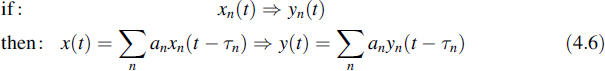
The definition of linearity of a system is as follows. Suppose a set of input signals {xn(t)} causes a corresponding set of output signals {yn(t)}. Then a system is said to be linear if any arbitrary linear combination of inputs causes the same linear combination of corresponding outputs, i.e.

with an arbitrary constants. In the notation of Equation (4.2),

A system is said to be time-invariant if a shift in time of the input causes a corresponding shift in the output. Therefore,

for arbitrary τ. Finally, a system is linear time-invariant (LTI) if it satisfies both conditions given by Equations (4.3) and (4.5), i.e.
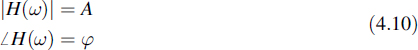
It can be proved [7] that complex exponential time functions, i.e. sine and cosine waves, are so-called eigenfunctions of linear time-invariant systems. An eigenfunction can physically be interpreted as a function that preserves its shape on transmission, i.e. a sine/cosine remains a sine/cosine, but its amplitude and/or phase may change. When these changes are known for all frequencies then the system is completely specified. This specification is done by means of the complex transfer function of the linear time-invariant system. If the system is excited with a complex exponential
and the corresponding output is
with A a real constant, then the transfer function equals

From Equations (4.7) to (4.9) the amplitude and the phase angle of the transfer function follow:
When in Equation (4.9), ω is given all values from −∞ to ∞, the transfer is completely known. As indicated in that equation the amplitude of the input x(t) is taken as unity and the phase zero for all frequencies. All observed complex values of y(t) are then presented by the function Y(ω). Since the input X(ω) was taken as unity for all frequencies, Equation (4.9) is in that case written as
From Fourier theory we know that the multiplication in the right-hand side of the latter equation is written in the time domain as a convolution [7,10]. Moreover, the inverse transform of 1 is a δ function. Since a δ function is also called an impulse, the time domain LTI system response following from Equation (4.11) is called the impulse response. We may therefore conclude that the system impulse response h(t) and the system transfer function H(ω) constitute a Fourier transform pair.
When the transfer function is known, the response of an LTI system to an input signal can be calculated. Provided that the input signal x(t) satisfies the Dirichlet conditions [10], its Fourier transform X(ω) exists. However, this frequency domain description of the signal is equivalent to decomposing the signal into complex exponentials, which in turn are eigenfunctions of the LTI system. This allows multiplication of X(ω) by H(ω) to find Y(ω), being the Fourier transform of output y(t); namely by taking the inverse transform of Y(ω), the signal y(t) is reconstructed from its complex exponential components. This justifies the use of Fourier transform theory to be applied to the transmission of signals through LTI signals. This leads us to the following theorem.
Theorem 6
If a linear time-invariant system with an impulse response h(t) is excited by an input signal x(t), then the output is
with the equivalent frequency domain description
where X(ω) and Y(ω) are the Fourier transforms of x(t) and y(t), respectively, and H(ω) is the Fourier transform of the impulse response h(t).
The two presentations of Equations (4.12) and (4.13) are so-called dual descriptions; i.e. both are complete and either of them is fully determined by the other one. If an important condition for physical realizability of the LTI system is taken into account, namely causality, then the impulse response will be zero for t < 0 and the lower bound of the integral in Equation (4.12) changes into zero.
This theorem is the main result we need to describe the filtering of stochastic processes by an LTI system, as is done in the sequel.
4.2 TIME DOMAIN DESCRIPTION OF FILTERING OF STOCHASTIC PROCESSES
Let us now consider the transmission of a stochastic process through an LTI system. Obviously, we may formally apply the time domain description given by Equation (4.12) to calculate the system response of a single realization of the ensemble. However, a frequency domain description is not always possible. Apart from the fact that realizations are often not explicitly known, it may happen that they do not satisfy the Dirichlet conditions. Therefore, we start by characterizing the filtering in the time domain. Later on the frequency domain description will follow from this.
4.2.1 The Mean Value of the Filter Output
The impulse response of the linear, time-invariant filter is denoted by h(t). Let us consider the ensemble of input realizations and call this input process X(t) and the corresponding output process Y(t). Then the relation between input and output is formally described by the convolution
When the input process X(t) is wide-sense stationary, then the mean value of the output signal is written as

where H(ω) is the Fourier transform of h(t). From Equation (4.15) it follows that the mean value of Y(t) equals the mean value of X(t) multiplied by the value of the transfer function for the d.c. component. This value is equal to the area under the curve of the impulse response function h(t). This conclusion is based on the property of X(t) at least being stationary of the first order.
4.2.2 The Autocorrelation Function of the Output
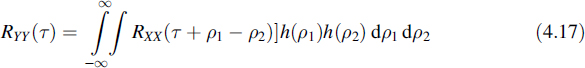
The autocorrelation function of Y(t) is found using the definition of Equation (2.13) and Equation (4.14):

Invoking X(t) as wide-sense stationary reduces this expression to
and the mean squared value of Y(t) reads
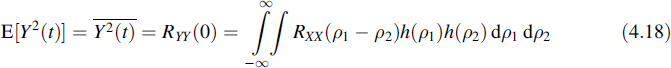
From Equations (4.15) and (4.17) it is concluded that Y(t) is wide-sense stationary when X(t) is wide-sense stationary, since neither the right-hand member of Equation (4.15) nor that of Equation (4.17) depends on t.
Equation (4.17) may also be written as
where the symbol * represents the convolution operation.
4.2.3 Cross-Correlation of the Input and Output
The cross-correlation of X(t) and Y(t) is found using Equations (2.46) and (4.14):

In the case where X(t) is wide-sense stationary Equation (4.20) reduces to
This expression may also be presented as the convolution of RXX(τ) and h(τ):
In a similar way the following expression can be derived:
From Equations (4.21) and (4.23) it is concluded that the cross-correlation functions do not depend on the absolute time parameter t. Earlier we concluded that Y(t) is wide-sense stationary if X(t) is wide-sense stationary. Now we conclude that X(t) and Y(t) are jointly wide-sense stationary if the input process X(t) is wide-sense stationary.
Substituting Equation (4.21) into Equation (4.17) reveals the relation between the autocorrelation function of the output and the cross-correlation between the input and output:
or, presented differently,
In a similar way it follows by substitution of Equation (4.23) into Equation (4.17) that
Example 4.1:
An important application of the cross-correlation function as given by Equation (4.22) consists of the identification of a linear system. If for the input process a white noise process, i.e. a process with a constant value of the power spectral density, let us say of magnitude N0/2, is selected then the autocorrelation function of that process becomes N0 δ(τ)/2. This makes the convolution very simple, since the convolution of a δ function with another function results in this second function itself. Thus, in that case the cross-correlation function of the input and output yields RXY(τ) = N0 h(τ)/2. Apart from a constant N0/2, the cross-correlation function equals the impulse response of the linear system; in this way we have found a method to measure this impulse response.
![]()
4.3 SPECTRA OF THE FILTER OUTPUT
In the preceding sections we described the output process of a linear time-invariant filter in terms of the properties of the input process. In doing so we used the time domain description. We concluded that in case of a wide-sense stationary input process the corresponding output process is wide-sense stationary as well, and that the two processes are jointly wide-sense stationary. This offers the opportunity to apply the Fourier transform to the different correlation functions in order to arrive at the spectral description of the output process and the relationship between the input and output processes. It must also be stressed that in this section only wide-sense stationary input processes will be considered.
The first property we are interested in is the spectral density of the output process. Using what has been derived in Section 4.2.2, this is easily revealed by transforming Equation (4.19) to the frequency domain. If we remember that the impulse response h(τ) is a real function and thus the Fourier transform of h(−τ) equals H*(ω), then the next important statement can be exposed.
Theorem 7
If a wide-sense stationary process X(t), with spectral density SXX(ω), is applied to the input of a linear, time-invariant filter with the transfer function H(ω), then the corresponding output process Y(t) is a wide-sense stationary process as well, and the spectral density of the output reads
The mean power of the output process is written as
Example 4.2:
Consider the RC network given in Figure 4.2. Then the voltage transfer function of this network is written as
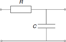
If we assume that the network is excited by a white noise process with spectral density of N0/2 and taking the modulus squared of Equation (4.29), then the output spectral density reads

For the power in the output process it is found that

![]()
In an earlier stage we found the power of a wide-sense stationary process in an alternative way, namely the value of the autocorrelation function at τ = 0 (see, for instance, Equation (4.16)). The power can also be calculated using that procedure. However, in order to be able to calculate the autocorrelation function of the output Y(t) we need the probability density function of X(t) in order to evaluate a double convolution or we need the probability density function of Y(t). Finding this latter function we meet two main obstacles: firstly, measuring the probability density function is much more difficult than measuring the power density function and, secondly, the probability density function of Y(t) by no means follows in a simple way from that of X(t). This latter statement has one important exception, namely if the probability density function of X(t) is Gaussian then the probability density function of Y(t) is Gaussian as well (see Section 2.3). However, calculating the mean and variance of Y(t), which are sufficient to determine the Gaussian density, using Equations (4.15) and (4.28) is a simpler and more convenient method.
From Equations (4.22) and (4.23) the cross-power spectra are deduced:
We are now in a position to give the proof of Equation (3.5). Suppose that SXX(ω) has a negative value for some arbitrary ω = ω0. Then a small interval (ω1, ω2) about ω0 is found, such that (see Figure 4.3(a))

Now consider an ideal bandpass filter with the transfer function (see Figure 4.3(b))
If the process X(t), with the power spectrum given in Figure 4.3(a), is applied to the input of this filter, then the spectrum of the output Y(t) is as presented in Figure 4.3(c) and is described by
so that
However, this is impossible as (see Equations (4.28) and (3.8))
This contradiction leads to the conclusion that the starting assumption SXX(ω) < 0 must be wrong.
4.4 NOISE BANDWIDTH
In this section we present a few definitions and concepts related to the bandwidth of a process or a linear, time-invariant system (filter).
4.4.1 Band-Limited Processes and Systems
A process X(t) is called a band-limited process if SXX(ω) = 0 outside certain regions of the ω axis. For a band-limited filter the same definition can be used, provided that SXX(ω) is replaced by H(ω). A few special cases of band-limited processes and systems are considered in the sequel.
- A process is called a lowpass process or baseband process if
- A process is called a bandpass process if (see Figure 4.4)
with
- A system is called a narrowband system if the bandwidth of that system is small compared to the frequency range over which the spectrum of the input process extends. A narrowband bandpass process is a process for which the bandwidth is much smaller than its central frequency, i.e. (see Figure 4.4)
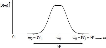
Figure 4.4 The spectrum of a bandpass process (only the region ω ≥ 0 is shown)
The following points should be noted:
- The definitions of processes 1 and 2 can also be used for systems if S(ω) is replaced by H(ω).
- In practical systems or processes the requirement that the spectrum or transfer function is zero in a certain region cannot exactly be met in a strict mathematical sense. Nevertheless, we will maintain the given names and concepts for those systems and processes for which the transfer function or spectrum has a negligibly low value in a certain frequency range.
- The spectrum of a bandpass process is not necessarily symmetrical about ω0.
4.4.2 Equivalent Noise Bandwidth
Equation (4.28) is often used for practical applications. For that reason there is a need for a simplified calculation method in order to compute the noise power at the output of a filter. In this section we will introduce such a simplification.
To that end consider a lowpass system with the transfer function H(ω). Assume that the spectrum of the input process equals N0/2 for all ω, with N0 a positive, real constant (such a spectrum is called a white noise spectrum). The power at the output of the filter is calculated using Equation (4.28):
Now define an ideal lowpass filter as
where WN is a positive constant chosen such that the noise power at the output of the ideal filter is equal to the noise power at the output of the original (practical) filter. WN therefore follows from the equation

If we consider |H(ω)|2 to be an even function of ω, then solving Equation (4.45) for WN yields
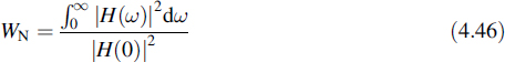

Figure 4.5 Equivalent noise bandwidth of a filter characteristic
WN is called the equivalent noise bandwidth of the filter with the transfer function H(ω). In Figure 4.5 it is indicated graphically how the equivalent noise bandwidth is determined. The solid curve represents the practical characteristic and the dashed line the ideal rectangular one. The equivalent noise bandwidth is such that in this picture the dashed area equals the shaded area.
From Equations (4.43) and (4.45) it follows that the output power of the filter can be written as
Thus, it can be shown for the special case of white input noise that the integral of Equation (4.43) is reduced to a product and the filter can be characterized by means of a single number WN as far as the noise filtering behaviour is concerned.
Example 4.3:
As an example of the equivalent noise bandwidth let us again consider the RC network presented in Figure 4.2. Using the definition of Equation (4.46) and the result of Example 4.2 (Equation (4.29)) it is found that WN = π/(2RC). This differs from the 3 dB bandwidth by a factor of π/2. It may not come as a surprise that the equivalent noise bandwidth of a circuit differs from the 3 dB bandwidth, since the definitions differ. On the other hand, both bandwidths are proportional to 1/(RC).
![]()
Equation (4.47) can often be used for the output of a narrowband lowpass filter. For such a system, which is analogous to Equation (4.43), the output power reads
and thus
The above calculation may also be applied to bandpass filters. Then it follows that

Here ω0 is a suitably chosen but arbitrary frequency in the passband of the bandpass filter, for instance the centre frequency or the frequency where |H(ω)| attains its maximum value. The noise power at the output is written as
When once again the input spectrum is approximately constant within the passband of the filter, which often happens in narrowband bandpass filters, then
In this way we end up with rather simple expressions for the noise output of linear time-invariant filters.
4.5 SPECTRUM OF A RANDOM DATA SIGNAL
This subject is dealt with here since for the derivation we need results from the filtering of stochastic processes, as dealt with in the preceding sections of this chapter. Let us consider the random data signal
where the data sequence is produced by making a random selection out of the possible values of A[n] for each moment of time nT. In the binary case, for example, we may have A[n]∈{−1, +1}. The sequence A[n] is supposed to be wide-sense stationary, where A[n] and A[k] in general will be correlated according to
The data symbols amplitude modulate the waveform p(t). This waveform may extend beyond the boundaries of a bit interval. The random data signal X(t) constitutes a cyclo-stationary process. We define a random variable Θ which is uniformly distributed on the interval (0, T] and which is supposed to be independent of the data A[n]; this latter assumption sounds reasonable. Using this random variable and the process X(t) we define the new process
Invoking Theorem 1 (see Section 2.2.2) we may conclude that this latter process is stationary. We model the process X(t) as resulting from exciting a linear time-invariant system having the impulse response h(t) = p(t) by the input process
The autocorrelation function of Y(t) is
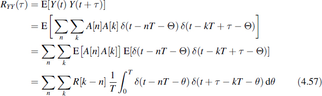
For all values of T, t, τ and n there will be only one single value of k for which both δ(t − nT − θ) and δ(t + τ − kT − θ) will be found in the interval 0 < θ ≤ T. This means that actually the integral in Equation (4.57) is the convolution of two δ functions, which is well defined (see reference [7]). Applying the basic definition of δ functions (see Appendix E) yields

where m = k − n. The autocorrelation function of Y(t) is presented in Figure 4.6. Finally, the autocorrelation function of X(t) follows:
The spectrum of the random data signal is found by Fourier transforming Equation (4.59):

Figure 4.6 The autocorrelation function of the process Y(t) consisting of a sequence of δ functions
where P(ω) is the Fourier transform of p(t). Using this latter equation and Equation (4.58) the following theorem can be stated.
Theorem 8
The spectrum of a random data signal reads

where R[m] are the autocorrelation values of the data sequence, P(ω) is the Fourier transform of the data pulses and T is the bit time.
This result, which was found by applying filtering to a stochastic process, is of great importance when calculating the spectrum of digital baseband or digitally modulated signals in communications, as will become clear from the examples in the sequel. When applying this theorem, two cases should clearly be distinguished, since they behave differently, both theoretically and as far as the practical consequences are concerned. We will deal with the two cases by means of examples.
Example 4.4:
The first case we consider is the situation where the mean value of X(t) is zero and consequently the autocorrelation function of the sequence A[n] has in practice a finite extent. Let us suppose that the summation in Equation (4.61) runs in that case from 1 to M.
As an important practical example of this case we consider the so-called polar NRZ signal, where NRZ is the abbreviation for non-return to zero, which reflects the behaviour of the data pulses. Possible values of A[n] are A[n] ∈ {+1, −1}, where these values are chosen with equal probability and independently of each other. For the signal waveform p(t) we take a rectangular pulse of width T, being the bit time. For the autocorrelation of the data sequence it is found that
Substituting these values into Equation (4.61) gives the power spectral density of the polar NRZ data signal:

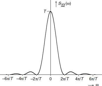
Figure 4.7 The power spectral density of the polar NRZ data signal
since the Fourier transform of the rectangular pulse is the well-known sinc function (see Appendix G). The resulting spectrum is shown in Figure 4.7.
The disadvantage of the polar NRZ signal is that it has a large value of its power spectrum near the d.c. component, although it does not comprise a d.c. component. On the other hand, the signal is easy to generate, and since it is a simplex signal (see Appendix A) it is power efficient.
![]()
Example 4.5:
In this example we consider the so-called unipolar RZ (return to zero) data signal. This once more reflects the behaviour of the data pulses. For this signal format the values of A[n] are chosen from the set A[n] ∈ {1, 0} with equal probability and mutually independent. The signalling waveform p(t) is defined by
It is easy to verify that the autocorrelation of the data sequence reads
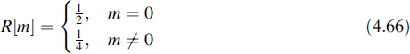
Inserting this result into Equation (4.61) reveals that we end up with an infinite sum of complex exponentials:
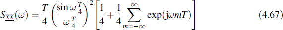

Figure 4.8 The power spectral density of the unipolar RZ data signal
However, this infinite sum of exponentials can be rewritten as

which is known as the Poisson sum formula [7]. Applying this sum formula to Equation (4.67) yields

This spectrum has been depicted in Figure 4.8. Comparing this figure with that of Figure 4.7 a few remarks need to be made. First of all, the first null bandwidth of the RZ signal increased by a factor of two compared to the NRZ signal. This is due to the fact that the pulse width was reduced by the same factor. Secondly, a series of δ functions appears in the spectrum. This is due to the fact that the unipolar signal has no zero mean. Besides the large value of the spectrum near zero frequency there is a d.c. component. This is also discovered from the δ function at zero frequency. The weights of the δ functions scale with the sinc function (Equation (4.69)) and vanish at all zero-crossings of the latter.
![]()
Theorem 8 is a powerful tool for calculating the spectrum of all types of formats for data signals. For more spectra of data signals see reference [6].
4.6 PRINCIPLES OF DISCRETE-TIME SIGNALS AND SYSTEMS
The description of discrete-time signals and systems follows in a straightforward manner by sampling the functions that describe their continuous counterparts. Especially for the theory and conversion it is most convenient to confine the procedure to ideal sampling, i.e. by multiplying the continuous functions by a sequence of δ functions, where these δ functions are equally spaced in time.
First of all we define the discrete-time δ function as follows:
or in general
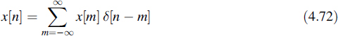
Based on this latter definition each arbitrary signal x[n] can alternatively be denoted as
We will limit our treatment to linear time-invariant systems. For discrete-time systems we introduce a similar definition for linear time-invariant systems as we did for continuous systems, namely

for any arbitrary set of constants ai, and mi.
Also, the convolution follows immediately from the continuous case

This latter description will be used for the output y[n] of a discrete-time system with the impulse response h[n], which has x[n] as an input signal. This expression is directly deduced by sampling Equation (4.12), but can alternatively be derived from Equation (4.72) and the properties of linear time-invariant systems.
In many practical situations the impulse response function h[n] will have a finite extent. Such filters are called finite impulse response filters, abbreviated as FIR filters, whereas the infinite impulse response filter is abbreviated to the IIR filter.
4.6.1 The Discrete Fourier Transform
For continuous signals and systems we have a dual frequency domain description. Now we look for discrete counterparts for both the Fourier transform and its inverse transform, since then these transformations can be performed by a digital processor. When considering for discrete-time signals the presentation by means of a sequence of δ functions
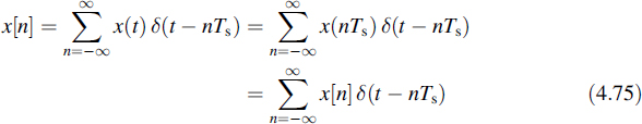
where 1/Ts is the sampling rate, the corresponding Fourier transform of the sequence x[n] is easily achieved, namely

Due to the discrete character of the time function its Fourier transform is a periodic function of frequency with period 2π/Ts. The inverse transform is therefore
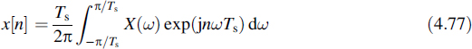
In Equations (4.76) and (4.77) the time domain has been discretized. Therefore, the operations are called the discrete-time Fourier transform (DTFT) and the inverse discrete-time Fourier transform (IDTFT), respectively. However, the frequency domain has not yet been discretized in those equations. Let us therefore now introduce a discrete presentation of ω as well. We define the radial frequency step as Δω ![]() 2π/T, where T still has to be determined. Moreover, the number of samples has to be limited to a finite amount, let us say N. In order to arrive at a self-consistent discrete Fourier transform this number has to be the same for both the time and frequency domains. Inserting this into Equation (4.76) gives
2π/T, where T still has to be determined. Moreover, the number of samples has to be limited to a finite amount, let us say N. In order to arrive at a self-consistent discrete Fourier transform this number has to be the same for both the time and frequency domains. Inserting this into Equation (4.76) gives

If we define the ratio of T and Ts as N ![]() T/Ts, then
T/Ts, then

Inserting the discrete frequency and limited amount of samples as defined above into Equation (4.77) and approximating the integral by a sum yields


The transform given by Equation (4.79) is called the discrete Fourier transform (abbreviated DFT) and Equation (4.81) is called the inverse discrete Fourier transform (IDFT). They are a discrete Fourier pair, i.e. inserting a sequence into Equation (4.79) and in turn inserting the outcome into Equation (4.81) results in the original sequence, and the other way around. In this sense the deduced set of two equations is self-consistent. It follows from the derivations that they are used as discrete approximations of the Fourier transforms. Modern mathematical software packages such as Matlab comprise special routines that perform the DFT and IDFT. The algorithms used in these packages are called the fast Fourier transform (FFT). The FFT algorithm and its inverse (IFFT) are just DFT, respectively IDFT, but are implemented in a very efficient way. The efficiency is maximum when the number of samples N is a power of 2. For more details on DFT and FFT see references [10] and [12].
Example 4.6:
It is well known from Fourier theory that the transform of a rectangular pulse in the time domain corresponds to a sinc function in the frequency domain (see Appendices E and G). Let us check this result by applying the FFT algorithm of Matlab to a rectangular pulse. Before programming the pulse, a few peculiarities of the FFT algorithm should be observed. First of all, it is only based on the running variables n and k, both running from 0 to N − 1, which means that no negative values along the x axis can be presented. Here it should be emphasized that in Matlab vectors run from 1 to N, which means that when applying this package the x axis is actually shifted over one position. Another important property is that since the algorithm both requires and produces N data values, Equations (4.79) and (4.81) are periodic functions of respectively k and n, and show a periodicity of N. Thanks to this periodicity the negative argument values can be displayed in the second half of the period. This actually means that in Figure 4.9(a) the rectangular time function is centred about zero. Similarly, the frequency function as displayed in Figure 4.9(b) is actually centred about zero as well. In this figure it has been taken that N = 256.
In Figure 4.10 the functions are redrawn with the second half shifted over one period to the left. This results in functions centred about zero in both domains and reflects the well-known result from Fourier theory. It will be clear that the actual time scale and frequency scale in this figure are to be determined based on the actual width of the rectangular pulse.
![]()
From a theoretical point of view it is impossible for both the time function and the corresponding frequency function to be of finite extent. However, one can imagine that if one of them is limited the parameters of the DFT are chosen such that the transform is a good approximation. Care should be taken with this, as shown in Figure 4.11. In this figure the rectangular pulse in the time domain has been narrowed, which results in a broader function in the frequency domain. In this case two adjacent periods in the frequency domain overlap; this is called aliasing.
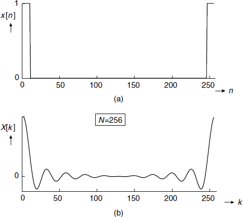
Figure 4.9 (a) The FFT applied to a rectangular pulse in the time domain; (b) the transform in the frequency domain
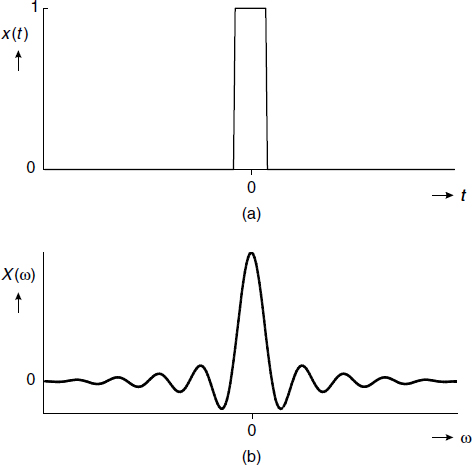
Figure 4.10 (a) The shifted rectangular pulse in the time domain; (b) the shifted transform in the frequency domain

Figure 4.11 (a) Narrowed pulse in the time domain; (b) the FFT result, showing aliasing
Although the two functions of Figure 4.11 form an FFT pair, the frequency domain result from Figure 4.11(b) shows a considerable distortion compared to the Fourier transform, which is rather well approximated by Figure 4.9(b). It will be clear that this aliasing can in such cases be prevented by increasing the number of samples N. This has to be done in this case by keeping the number of samples of value 1 the same, and inserting extra zeros in the middle of the interval.
4.6.2 The z-Transform
An alternative approach to deal with discrete-time signals and systems is by setting exp(jωTs) ![]() z in Equation (4.76). This results in the so-called z-transform, which is defined as
z in Equation (4.76). This results in the so-called z-transform, which is defined as
Comparing this with Equation (4.76) it is concluded that
Since Equation (4.82) is exactly the same as the discrete Fourier transform, only a different notation has been introduced, the same operations used with the Fourier transform are allowed. If we consider Equation (4.82) as the z-transform of the input signal to a linear time-invariant discrete-time system, when calculating the z-transform of the impulse response

the z-transform of the output is found to be
A system is called stable if it has a bounded output signal when the input is bounded. A discrete-time system is a stable system if all the poles of ![]() (z) lie inside the unit circle of the z plane or in terms of the impulse response [10]:
(z) lie inside the unit circle of the z plane or in terms of the impulse response [10]:

The z-transform is a very powerful tool to use when dealing with discrete-time signals and systems. This is due to the simple and compact presentation of it on the one hand and the fact that the coefficients of the different powers z−n are identified as the time samples at nTs on the other hand. For further details on the z-transform see references [10] and [12].
Example 4.7:
Consider a discrete-time system with the impulse response
and where |a| < 1. The sequence h[n] has been depicted in Figure 4.12 for a positive value of a. The z-transform of this impulse response is
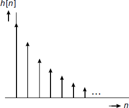
Figure 4.12 The sequence an with 0 < a < 1
Let us suppose that this filter is excited with an input sequence
with |b| < 1 and b ≠ a. Similar to Equation (4.88) the z-transform of this sequence is
Then the z-transform of the output is
The time sequence can be recovered from this by decomposition into partial fractions:
From this the output sequence is easily derived:

![]()
As far as the realization of discrete-time filters is concerned two main types are distinguished, namely the non-recursive filter structure and the recursive. The realization of the non-recursive filter is quite straightforward and the structure is given in Figure 4.13; it is also called the transversal filter or tapped delay line filter. The boxes represent delays of Ts seconds and the outputs are multiplied by an. The delayed and multiplied outputs are added to form the filter output sequence y[n]. It is easy to understand that the transfer function of the filter in the z domain is described by the polynomial
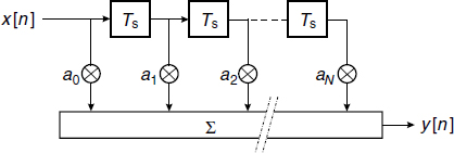
Figure 4.13 The structure of the discrete-time non-recursive filter, transversal filter or tapped delay line filter

Figure 4.14 The structure of the discrete-time recursive filter

From the structure it follows that it is a finite impulse response (FIR) filter and there is a simple and direct relation between the multiplication factors and the polynomial coefficients. An FIR filter is inherently stable.
The recursive filter is based on a similar tapped delay line filter, which is in a feedback loop depicted in Figure 4.14. The transfer function of the feedback filter is
and from the figure it is easily derived that the transfer function of the recursive filter is
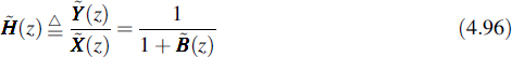
As a rule this transfer function has an infinite impulse response, so it is an IIR filter. The stability of the recursive filter is guaranteed if the denominator polynomial 1 + ![]() (z) in Equation (4.96) has no zeros outside the unit circle.
(z) in Equation (4.96) has no zeros outside the unit circle.
In filter synthesis the transfer function is often specified by means of a rational function; i.e. it is given as

It can be seen that this function is realizable as the cascade of the FIR filter from Figure 4.13 and the IIR filter from Figure 4.14, as follows from Equations (4.94) to (4.96), while the same stability criterion is valid as for the IIR filter.
The Signal Processing Toolbox from Matlab comprises several commands for the analysis and design of discrete-time filters, one of which is filter, which calculates the output of filters described by Equation (4.97) when excited by a specified input sequence.
4.7 DISCRETE-TIME FILTERING OF RANDOM SEQUENCES
4.7.1 Time Domain Description of the Filtering
The filtering of a discrete-time stochastic process X[n] by a discrete-time linear time-invariant system with the impulse response h[n] is described by the convolution (see Equation (4.74))

It should be remembered that treatment is confined to real wide-sense stationary processes. Then the mean value of the output sequence is

where ![]() (1) is the z-transform of h[n] evaluated at z = 1, which follows from its definition (see Equation (4.84)).
(1) is the z-transform of h[n] evaluated at z = 1, which follows from its definition (see Equation (4.84)).
The autocorrelation sequence of the output process, which can be proved to be wide-sense stationary as well, is

The cross-correlation sequence between the input and output becomes

In a similar way is derived
Moreover, the following relation exists:
4.7.2 Frequency Domain Description of the Filtering
Once the autocorrelation sequence at the output of the linear time-invariant discrete-time system is known, the spectrum at the output follows from Equation (4.100):
where the functions of frequency have to be interpreted as in Equation (4.76).
Using the z-transform, and assuming h[n] to be real, we arrive at
since for a real system H*(ω) = H(−ω) and consequently ![]() (z) =
(z) = ![]() (z−1).
(z−1).
Owing to the discrete-time nature of Y[n] its spectrum is periodic. According to Equation (3.66) its power is denoted by
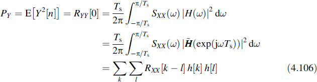
The last line of this equation follows from Equation (4.100).
Example 4.8:
Let us consider the system with the z-transform
with |a| < 1; this is the system introduced in Example 4.7. We assume that the system is driven by the stochastic process X[n] with spectral density ![]() XX(z) = 1 or equivalently RXX [m] = δ[m]; later on we will call such a process white noise. Then the output spectral density according to Equation (4.105) is written as
XX(z) = 1 or equivalently RXX [m] = δ[m]; later on we will call such a process white noise. Then the output spectral density according to Equation (4.105) is written as

Expanding this expression in partial fractions yields
Next we expand in series the fractions with z and z−1:
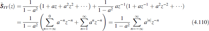
The autocorrelation sequence of the output is easily derived from this, namely
and in turn it follows immediately that
The power spectrum is deduced from Equation (4.109), which for that purpose is rewritten as
Inserting z = exp(jωTs) leads to the spectrum in the frequency domain
In Figure 4.15 this spectrum has been depicted for a = 0.8 and a sampling interval time of 1 second. As a consequence the spectrum has a periodicity of 2π in the angular frequency domain. Clearly, this is a lowpass spectrum.
![]()
From this example it is concluded that the z-transform is a powerful tool for analysing discrete-time systems that are driven by a stochastic process. The transformation and its inverse are quite simple and the operations in the z domain are simply algebraic manipulations. Moreover, conversion from the z domain to the frequency domain is just a simple substitution.
Matlab comprises the procedures conv and deconv for multiplication and division of polynomials, respectively. The filter command in the Signal Processing Toolbox can do the same job (see also the end of Subsection 4.6.2). Moreover, the same toolbox comprises the command freqz, which, apart from the filter operation, also converts the result to the frequency domain.
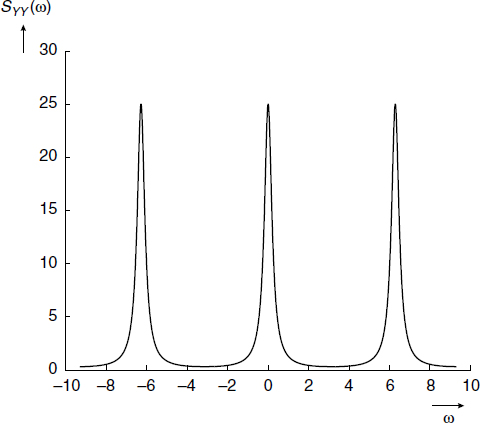
Figure 4.15 The periodic spectrum of the example with a = 0.8
4.8 SUMMARY
The input of a linear time-invariant system is excited with a wide-sense stationary process. In the time domain the output process is described as the convolution of the input process and the impulse response of the system, e.g. a filter. Next from this description such characteristics as mean value and correlation functions are to be determined, using the definitions given in Chapter 2. Although the expression for the autocorrelation function of the output process looks rather complicated, namely a twofold convolution, for certain processes this may result in a tractable description. Applying the Fourier transform and arriving at the power spectral density produces a much simpler expression. The probability density function of the output process can, in general, not be easily determined in analytical form from the input probability density function. There is an important exception for this; namely if the input process has a Gaussian probability density function then the output process also has a Gaussian probability density function.
The concept of equivalent noise bandwidth has been defined in order to arrive at an even more simple description of noise filtering in the frequency domain. The theory of noise filtering is applied to a specific stochastic process in order to describe the autocorrelation function and spectrum of random data signals.
Next, attention is paid to discrete-time signals and systems. Specials tools for that are dealt with. The discrete Fourier transform (DFT) and its inverse (IDFT) are derived and it is shown that this transform can serve as an approximation of the Fourier transform. Problems when applying the DFT for that purpose are indicated, including the ways used to avoid them. A closely related transform, namely the z-transform, appears to be more tractable for practical applications. The relation to the Fourier transform is quite simple. Finally, it is shown how to apply these transforms to filtering discrete-time processes by discrete-time systems.
4.9 PROBLEMS
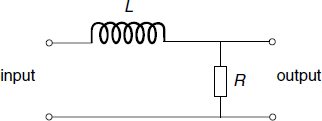
4.1 Consider the network given in Figure 4.16.
(a) Calculate the voltage transfer function. Make a plot of its absolute value on a double logarithmic scale using Matlab and with R/L = 1.
(b) Calculate the impulse response. Make a plot of it using Matlab.
(c) Calculate the response of the network to a rectangular input pulse that starts at t = 0, has height 1 and lasts for 2 seconds. Make a plot of the response using Matlab.
4.2 Derive the Fourier transform of the function
![]()
Use Matlab to produce a plot of the transform with α = 1 and ω0 = 10.
4.3 Consider the circuit given in Figure 4.17.
(a) Determine the impulse response of the circuit. Make a sketch of it.
(b) Calculate the transfer function H(ω).
(c) Determine and draw the response y(t) to the input signal x(t) = A rect ![]() , where A is a constant. (See Appendix E for the definition of the rectangular pulse function rect(·)).
, where A is a constant. (See Appendix E for the definition of the rectangular pulse function rect(·)).
(d) Determine and draw the response y(t) to the input signal x(t) = A rect ![]() , where A is a constant.
, where A is a constant.
4.4 A stochastic process X(t) = A sin(ω0t − Θ) is given, with A and ω0 real, positive constants and Θ a random variable that is uniformly distributed on the interval (0, 2π]. This process is applied to a linear time-invariant network with the impulse response h(t) = u(t) exp(−t/τ0). (The unit-step function u(t) is defined in Appendix E.) Here τ0 is a positive, real constant. Derive an expression for the output process.

4.5 A wide-sense stationary Gaussian process with spectral density N0/2 is applied to the input of a linear time-invariant filter. The impulse response of the filter is
![]()
(a) Sketch the impulse response of the filter.
(b) Calculate the mean value and the variance of the output process.
(c) Determine the probability density function of the output process.
(d) Calculate the autocorrelation function of the output process.
(e) Calculate the power spectrum of the output process.
4.6 A wide-sense process X(t) has the autocorrelation function RXX(τ) = A2 + B(1 − |τ|/T) for |τ| < T and with A, B and T positive constants. This process is used as the input to a linear, time-invariant system with the impulse response h(t) = u(t) − u(t − T).
(a) Sketch RXX(τ) and h(t).
(b) Calculate the mean value of the output process.
4.7 White noise with spectral density of N0/2 V2/Hz is applied to the input of the system given in Problem 4.1.
(a) Calculate the spectral density of the output.
(b) Calculate the mean quadratic value of the output process.
4.8 Consider the circuit in Figure 4.18, where X(t) is a wide-sense stationary voltage process. Measurements on the output voltage process Y(t) reveal that this process is Gaussian. Moreover, it is measured as
![]()
(a) Determine the probability density function fY(y). Plot this function using Matlab.
(b) Calculate and sketch the spectrum SXX(ω) of the input process.
(c) Calculate and sketch the autocorrelation function RXX(τ) of the input process.

4.9 Two linear time-invariant systems have impulse responses of h1(t) and h2(t), respectively. The process X1(t) is applied to the first system and the corresponding response reads Y1(t). Similarly, the input process X2(t) to the second system results in the response Y2(t). Calculate the cross-correlation function of Y1(t) and Y2(t) in terms of h1(t), h2(t) and the cross-correlation function of X1(t) and X2(t), assuming X1(t) and X2(t) to be jointly wide-sense stationary.
4.10 Two systems are cascaded. A stochastic process X(t) is applied to the input of the first system having the impulse response h1(t). The response of this system is W(t) and serves as the input of the second system with the impulse response h2(t). The response of this second system reads Y(t). Calculate the cross-correlation function of W(t) and Y(t) in terms of h1(t) and h2(t), and the autocorrelation function of X(t). Assume that X(t) is wide-sense stationary.
4.11 The process (called the signal) X(t) = cos(ω0t − Θ), with Θ uniformly distributed on the interval (0, 2π], is added to white noise with spectral density N0/2. The sum is applied to the RC network given in Figure 4.2.
(a) Calculate the power spectral densities of the output signal and the output noise.
(b) Calculate the ratio of the mean output signal power and the mean output noise power, the so-called signal-to-noise ratio.
(c) For what value of τ0 = RC does this ratio become maximal?
4.12 White noise with spectral density of N0/2 is applied to the input of a linear time-invariant system with the transfer function H(ω) = (1 + jωτ0)−2. Calculate the power of the output process.
4.13 A differentiating network may be considered as a linear time-invariant system with the transfer function H(ω) = jω. If the input is a wide-sense stationary process X(t), then the output process is dX(t)/dt = ![]() . Show that:
. Show that:
(a) ![]()
(b) ![]()
4.14 To the differentiating network presented in Problem 4.13 a wide-sense stationary process X(t) is applied. The corresponding output process is Y(t).
(a) Are the random variables X(t) and Y(t), both considered at the same fixed time t, orthogonal?
(b) Are these random variables uncorrelated?
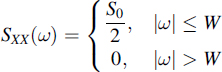
4.15 A stochastic process with the power spectral density of
![]()
is applied to a differentiating network.
(a) Find the power spectral density of the output process.
(b) Calculate the power of the derivative of X(t).
4.16 Consider the stochastic process
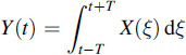
where X(t) is a wide-sense stationary process.
(a) Design a linear time-invariant system that produces the given relation between its input process X(t) and the corresponding output process Y(t).
(b) Express the autocorrelation function of Y(t) in terms of that for X(t).
(c) Express the power spectrum of Y(t) in terms of that for X(t).
4.17 Reconsider Problem 4.16.
(a) Prove that the given integration can be realized by a linear time-invariant filter with an impulse response rect[t/(2T)].
(b) Fill an array in Matlab with a harmonic function, let us say a cosine. Take, for example, 10 cycles of 1/(2π) Hz and increments of 0.01 for the time parameter. Plot the function.
(c) Generate a Gaussian noise wave with mean of zero and unit variance, and of the same length as the cosine using the Matlab command randn, add this wave to the cosine and plot the result. Note that each time you run the program a different wave is produced.
(d) Program a vector consisting of all ones. Convolve this vector with the cosine plus noise vector and observe the result. Take different lengths, e.g. equivalent to 2T = 0.05, 0.10 and 0.20. Explain the differences in the different curves.
4.18 In FM detection the white additive noise is converted into noise with spectral density
![]()
and assume that this noise is wide-sense stationary. Suppose that the signal spectrum is
and that in the receiver the detected signal is filtered by an ideal lowpass filter of bandwidth W.
(a) Calculate the signal-to-noise ratio.
In audio FM signals so-called pre-emphasis and de-emphasis filtering is applied to improve the signal-to-noise ratio. To that end prior to modulation and transmission the audio baseband signal is filtered by the pre-emphasis filter with the transfer function
![]()
At the receiver side the baseband signal is filtered by the de-emphasis filter such that the spectrum is once more flat and equal to S0/2.
(b) Make a block schematic of the total communication scheme.
(c) Sketch the different signal and noise spectra.
(d) Calculate the improvement factor of the signal-to-noise ratio.
(e) Evaluate the improvement in dB for the practical values: W/(2π) = 15 kHz, Wp/(2π) = 2.1 kHz.
4.19 A so-called nth-order Butterworth filter is defined by the squared value of the amplitude of the transfer function
![]()
where n is an integer, which is called the order of the filter. W is the −3 dB bandwidth in radians per second.
(a) Use Matlab to produce a set of curves that present this squared transfer as a function of frequency; plot the curves on a double logarithmic scale for n = 1,2,3,4.
(b) Calculate and evaluate the equivalent noise bandwidth for n = 1 and n = 2.
4.20 For the transfer function of a bandpass filter it is given that
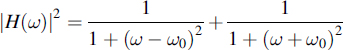
(a) Use Matlab to plot |H(ω)|2 for ω0 = 10.
(b) Calculate the equivalent noise bandwidth of the filter.
(c) Calculate the output noise power when wide-sense stationary noise with spectral density of N0/2 is applied to the input of this filter.
4.21 Consider the so-called Manchester (or split-phase) signalling format defined by
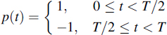
where T is the bit time. The data symbols A[n] are selected from the set {1, −1} with equal probability and are mutually independent.
(a) Sketch the Manchester coded signal of the sequence 1010111001.
(b) Calculate the power spectral density of this data signal. Use Matlab to plot it.
(c) Discuss the properties of the spectrum in comparison to the polar NRZ signal.
4.22 In the bipolar NRZ signalling format the binary 1's are alternately mapped to A[n] = +1 volt and A[n] = −1 volt. The binary 0 is mapped to A[n] = 0 volt. The bits are selected with equal probability and are mutually independent.
(a) Sketch the bipolar NRZ coded signal of the sequence 1010111001.
(b) Calculate the power spectral density of this data signal. Use Matlab to plot it.
(c) Discuss the properties of the spectrum in comparison to the polar NRZ signal.
4.23 Reconsider Example 4.6. Using Matlab fill in an array of size 256 with a rectangular function of width 50. Apply the FFT procedure to that. Square the resulting array and subsequently apply the IFFT procedure.
(a) Check the FFT result for aliasing.
(b) What in the time domain is the equivalence of squaring in the frequency domain?
(c) Check the IFFT result with respect to your answer to (b).
Now fill another array of size 256 with a rectangular function of width 4 and apply the FFT to it.
(d) Check the result for aliasing.
(e) Multiply the FFT result of the 50 wide pulse by that of the 4 wide pulse and IFFT the multiplication. Is the result what you expected in view of the result from (d)?
4.24 In digital communications a well-known disturbance of the received data symbols is the so-called intersymbol interference (see references [6], [9] and [11]). It is actually the spill-over of the pulse representing a certain bit to the time interval assigned to the adjacent pulses that represent different bits. This disturbance is a consequence of the distortion in the transmission channel. By means of proper filtering, called equalization, the intersymbol interference can be removed or minimized. Assume that each received pulse that represents a bit is sampled once and that the sampled sequence is represented by its z-transform ![]() (z). For an ideal channel, i.e. a channel that does not produce intersymbol interference, we have
(z). For an ideal channel, i.e. a channel that does not produce intersymbol interference, we have ![]() (z) = 1.
(z) = 1.
Let us now consider a channel with intersymbol interference and design a discrete-time filter that equalizes the channel. If the z-transform of the filter impulse response is denoted by ![]() (z), then for the equalized pulse the condition
(z), then for the equalized pulse the condition ![]() (z)
(z) ![]() (z) = 1 should be satisfied. Therefore, in this problem the sequence
(z) = 1 should be satisfied. Therefore, in this problem the sequence ![]() (z) is known and the sequence
(z) is known and the sequence ![]() (z) has to be solved to satisfy this condition. It appears that the Matlab command deconv is not well suited to solving this problem.
(z) has to be solved to satisfy this condition. It appears that the Matlab command deconv is not well suited to solving this problem.
(a) Suppose that ![]() (z) comprises three terms. Show that the condition for equalization is equivalent to
(z) comprises three terms. Show that the condition for equalization is equivalent to

(b) Consider a received pulse ![]() (z) = 0.1z + 1 − 0.2z−1 + 0.1z−2. Design the equalizer filter of length 3.
(z) = 0.1z + 1 − 0.2z−1 + 0.1z−2. Design the equalizer filter of length 3.
(c) As the quality factor with respect to intersymbol interference we define the ‘worst case interference’. It is the sum of the absolute signal samples minus the desired sample value 1. Calculate the output sequence of the equalizer designed in (b) using conv and calculate its worst-case interference. Compare this with the unequalized worst-case interference.
(d) Redo the equalizer design for filter lengths 5 and 7, and observe the change in the worst-case interference.
4.25 Find the transfer function and filter structure of the discrete-time system when the following relations exist between the input and output:
(a) y[n] + 2y[n − 1] + 0.5y[n − 2] = x[n] = x[n − 2]
(b) 4y[n] + y[n − 1] − 2y[n − 2] − 2y[n − 3] = x[n] + x[n − 1] − x[n − 2]
(c) Are the given systems stable?
Hint: use the Matlab command roots to compute the roots of polynomials.
4.26 White noise with spectral density of N0/2 is applied to an ideal lowpass filter with bandwidth W.
(a) Calculate the autocorrelation function of the output process. Use Matlab to plot this function.
(b) The output noise is sampled at the time instants tn = nπ/W with n integer. What can be remarked with respect to the sample values?
4.27 A discrete-time system has the transfer function ![]() (z) = 1 + 0.9z−1 + 0.7z−2. To the input of the system the signal with z-transform
(z) = 1 + 0.9z−1 + 0.7z−2. To the input of the system the signal with z-transform ![]() (z) = 0.7 + 0.9z−1 + z−2 is applied. This signal is disturbed by a wide-sense stationary white noise sequence. The autocorrelation sequence of this noise is RNN[m] = 0.01 δ[m].
(z) = 0.7 + 0.9z−1 + z−2 is applied. This signal is disturbed by a wide-sense stationary white noise sequence. The autocorrelation sequence of this noise is RNN[m] = 0.01 δ[m].
(a) Calculate the signal output sequence.
(b) Calculate the autocorrelation sequence at the output.
(c) Calculate the maximum value of the signal-to-noise ratio. At what moment in time will that occur?
Hint: you can eventually use the Matlab command conv to perform the required polynomial multiplications. In this way the solution found using pencil and paper can be checked.
4.28 The transfer function of a discrete-time filter is given by
![]()
(a) Use Matlab's freqz to plot the absolute value of the transfer function in the frequency domain.
(b) If the discrete-time system operates at a sampling rate of 1 MHz and a sine wave of 50 kHz and an amplitude of unity is applied to the filter input, compute the power of the corresponding output signal.
(c) A zero mean white Gaussian noise wave is added to the sine wave at the input such that the signal-to-noise ratio amounts to 0 dB. Compute the signal-to-noise ratio at the output.
(d) Use the Matlab command randn to generate the noise wave. Design and implement a procedure to test whether the generated noise wave is indeed approximately white noise.
(e) Check the analytical result of (c) by means of proper operations on the waves that are generated by Matlab.
Introduction to Random Signals and Noise W. van Etten
© 2005 John Wiley & Sons, Ltd